Power System Event Classification and Localization Using a Convolutional Neural Network

Detection and timely identification of power system disturbances are essential for situation awareness and reliable electricity grid operation. Because records of actual events in the system are limited, ensemble simulation-based events are needed to provide adequate data for building event-detection models through deep learning; e.g., a convolutional neural network (CNN). An ensemble numerical simulation-based training data set have been generated through dynamic simulations performed on the Polish system with various types of faults in different locations. Such data augmentation is proven to be able to provide adequate data for deep learning. The synchronous generators’ frequency signals are used and encoded into images for developing and evaluating CNN models for classification of fault types and locations. With a time-domain stacked image set as the benchmark, two different time-series encoding approaches, i.e., wavelet decomposition-based frequency-domain stacking and polar coordinate system-based Gramian Angular Field (GAF) stacking, are also adopted to evaluate and compare the CNN model performance and applicability. The various encoding approaches are suitable for different fault types and spatial zonation. With optimized settings of the developed CNN models, the classification and localization accuracies can go beyond 84 and 91%, respectively.

Introduction

More and more digital sensors, e.g., synchronized phasor measurements units (PMUs) and digital fault recorders have been deployed in the electricity system to monitor, control and protect the power grid (Gopakumar et al., 2018). PMUs provide high-resolution, accurate, and time-synchronized information about power system state and dynamics. With the variety of signals from the many various sensors, digital signal processing plays an important role in improving system stability and reliability (Grigsby, 2016; Ren et al., 2018a; Ren et al., 2018b). Power system faults can be caused by several factors, including equipment, operation, human interference, weather conditions, and the environment (Han and Zhou, 2016). Effective fault detection and identification are needed to improve system reliability, prevent widespread damage to the power system network, and avoid power system blackouts (Guillen et al., 2015; Alhelou et al., 2018). Locating a faulty zone (area) can also help improve power system situational awareness and help crews take proper corrective actions (Gopakumar et al., 2015; Yusuff et al., 2011).

Nowadays, great efforts have been made in developing new methodologies, from both data and model perspectives, for fault detection and isolation (FDI) (Chen and Patton, 2012; Costamagna et al., 2015; Jan et al., 2017; Zhang et al., 2016; Alhelou et al., 2018). Data-driven FDI has received significant attention recently; for example, approaches using deep learning techniques such as long short-term memory (LSTM) networks and convolutional neural networks (CNNs) are popular among the deep neural networks (Chen et al., 2017; Zhang et al., 2017; Patil et al., 2019; Paul and Mohanty, 2019; Qu et al., 2020). An LSTM network (Hochreiter and Schmidhuber, 1997) has advantages for learning sequences containing both short- and long-term patterns from time series (Malhotra et al., 2015), while CNN is a commodity in the computer vision field that is capable of achieving record-breaking results on highly challenging image datasets (Krizhevsky et al., 2012; Zhu et al., 2018). With limited data preprocessing, convolutional layers in CNN can serve as dimension reduction model which have the power to obtain effective representations of the raw images through increasing depth and width of model without increasing the computational demands (Gu et al., 2018). Many advanced multi-class–classification CNNs have been reported, e.g., in the ImageNet challenge, with high accuracy scores (Canziani et al., 2016; Russakovsky et al., 2015), as well as other breakthroughs on computer vision tasks such as image segmentation, object detection, speech and natural language processing (Sermanet et al., 2013; Zeiler and Fergus, 2014; He et al., 2016; Tan and Le, 2019; Shorten and Khoshgoftaar, 2019).

Monitoring time series obtained from power systems can be transformed into two-dimensional (2D) images for better visualization, and to take advantage of the successful image-based deep learning architectures in computer vision to learn and extract features and structure in multivariate time series. Several methods have been used for encoding and stacking time series, as explained below. Frequency-based wavelet decomposition has been used in speed and image processing as well as time series analysis. A discrete wavelet transform (DWT) is sufficient to decompose and reconstruct most power quality problems, and can adequately and efficiently provide information, in a hierarchical detail structure in high frequency and approximations in low frequency. DWT has the capability to obtain both temporal and frequency information on the signals through effective time localization of all frequency components (Mallat, 1989). These capabilities are inherent to dealing with the time series and signals, and have been applied in multiple studies, including the power system (Saleh et al., 2008; Avdakovic et al., 2012; Livani and Evrenosoğlu, 2012). Previous studies have implemented feature extractions from power waveform as inputs for data-driven approaches, where CNN achieved a high model accuracy on event classification and anomaly detection (Wang et al., 2019; Basumallik et al., 2019). The Gramian Angular Field (GAF) is another recent encoding approach for converting time series data into RGB images using a Gramian matrix (Wang and Oates, 2015a). Recently this approach was used to convert signals through GAF and detect the features successfully in other domain studies, but rarely in the power system (Wang and Oates, 2015b; Zhang et al., 2019; Thanaraj et al., 2020). Given the successful implementation of different time series encoding techniques and CNN models in the power system studies, we aim to develop and evaluate CNN models for classification and localization of various types of faults and the impacts of the time series encoding approaches for predicting power system disturbances.

Observation-based event detection, classification, and localization using real world data are usually challenging because labeled data is often lacking. Such data inadequacy cannot support training of deep neural networks. One solution is use of data augmentation by generating an ensemble simulation-based training data set. In this study, we evaluated the feasibility of using ensemble simulation-based data with various types of faults; this will provide adequate labeled data for supervised learning. Dynamic simulations were performed on a MATPOWER Polish 3120-bus system with four types of faults in five geophysical zones. The multichannel time series of machine speed data were extracted and encoded to images for evaluating the feasibility of CNN models for classification (fault types) and localization (occurrence zones). Time series stacking is straightforward, and it requires the fewest computational resources; it served as the benchmark dataset for our proposed CNN model. Three other time-series encoding approaches, i.e., time-domain stacking, wavelet decomposition-based frequency-domain stacking, and polar coordinate system-based GAF stacking, were adopted to evaluate and compare performance of the CNN models. Visual Geometry Group (VGG) model architecture was adopted in our CNN to push the model depth toward high accuracy (Simonyan and Zisserman, 2014).

Power System Test Bed and Dynamic Simulation

Polish System

Simulation tests were performed on the 3120-bus Polish system (“case3120sp.m”) (MATPOWER, 2008). Dynamic data have been developed in Siemens PSS®E (PSS/E) format that include generator, governor, stabilizer, and exciter models for generator dynamics. Several protection models were also prepared in PSS/E format; these include protection models that incorporate distance relays, generator-based voltage and frequency relays, and underfrequency and undervoltage load-shedding relays. They were added to the existing relay protection models in the Polish case. The Polish system has 3,120 buses, 3,487 branches, 2,314 loads, and 505 generators and comprises five zones. The zonal model for total generation of each zone and the connections between zones are illustrated in Figure 1. Zone 3 is the largest zone connected with Zones 1, 2, and 4. Zone 5 is the smallest zone, with only 841 MW; it is connected only with Zones 1 and 4.

FIGURE 1

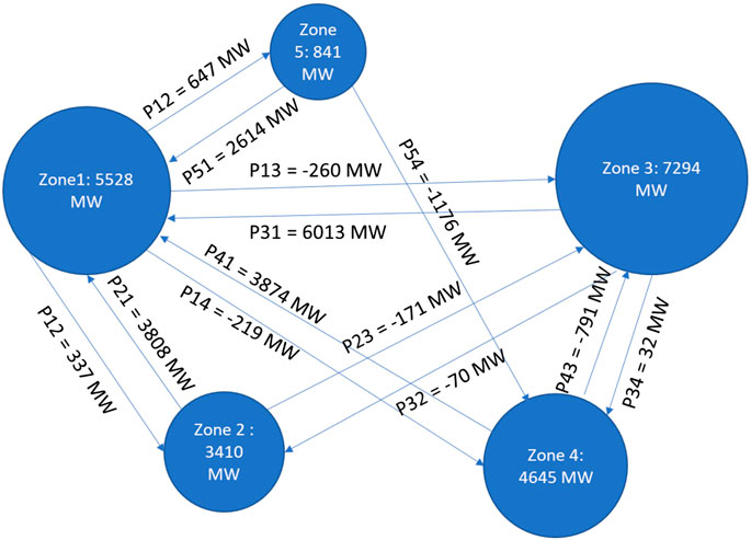
FIGURE 1. Zonal model of the Polish 3120-bus system.

Fault Types and Implementation

Various power system faults were simulated using the PSS/E software. These faults can be categorized into four types, and the outage characteristics of each type have been summarized in Table 1. Fault 1 is the single generator and multiple line fault. In this scenario, each generator and consequently two transmission lines were tripped in the system. A total of 298 contingencies were simulated for Fault 1. For Fault 2, a three-phase fault at a bus during dynamic simulations was applied to the Polish system with 3,120 contingencies. Different generators were set to be tripped during dynamic simulation for the system, as Faults 3 and 4, with 298 contingencies for each fault type. In Fault 3, each generator was put out-of-service and Fault 4 has the two neighboring generators out-of-service.

TABLE 1

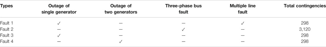
TABLE 1. Fault types simulated in Polish system.

Methodology

Wavelet Decomposition

The wavelet decomposition is a mathematical tool to analyze signals in both time and frequency domains at multiple resolution levels. For a time series $X\left(t\right)$, the wavelet transform is defined as shown in Eq. 1 with a given wavelet function $\psi \left(t\right)$. $\psi \left(t\right)$ is called a mother wavelet, chosen from the broad wavelet family, which includes Haar, Morlet, B-Spline, Mexican hat, and Daubechies families, among others. $W_x\left(a, b\right)$ is the wavelet coefficient at different resolution levels with respect to time.

$W_x\left(a, b\right)= {\left|a\right|}^{-\frac{1}{2}}\underset{-\infty }{\overset{\infty }{{\displaystyle \int }}}X\left(t\right)\overline{\psi }\left(\raisebox{1ex}{$t-b$}\!\left/ \!\raisebox{-1ex}{$a$}\right.\right)dt(1)$

In practice, because the time series are discrete, the DWT can be obtained by discretizing the scale parameter $a$ and location parameter $b$. At decomposition level $j (j=1, 2, 3, \dots n)$, discretizing $a$ = $2_j$ and $b$ = $k{2}_j$ yield orthonormal basis functions for certain choices of $\psi ,$ as expressed in Eq. 2, where $k$ is the time translation factor. This results in high frequency resolution at low frequencies and high time resolution at high frequencies, removing the redundant information.

${\psi }_{\left(j, k\right)}\left(t\right)= 2^{-\frac{j}{2}}\psi (2^{-j}t-k)(2)$

The DWT provides the diagnosis decomposition of a given time series $X\left(t\right)$ into a progression of low-frequency approximations and high-frequency details expressed as follows:

$X\left(t\right)= D_1+D_2+ D_3+\dots + D_n+A_n(3)$

Where $D_1$, $D_2$, $D_3$,…, $D_n$ are the detail coefficient sets and $A_n$ represents the approximation coefficient sets at the level n. The output of the DWT is sensitive to the wavelet faction. In our study, the Morlet wavelet was adopted to capture time-varying frequency and amplitude in time series (Grossmann and Morlet, 1984). It is a complex sine wave tapered by a Gaussian function. The parameter that defines the time–frequency precision trade-off is referred to as the “number of cycles.”

Gramian Angular Field

For a time series $X=\{x_1, x_2, x_3,\dots , x_n\}$ with length $n$, the first step is to rescale $X$ to the interval [−1, 1] using Eq. 4.

$\widetilde{x_t}= \raisebox{1ex}{$(x_t-\max \left(X\right)+(x_t-\text{min}(X))$}\!\left/ \!\raisebox{-1ex}{$\max \left(X\right)-\min (X)$}\right. ,t=1, 2, 3,\dots , n(4)$

Then the rescaled time series $\tilde{X}$ is converted to polar coordinates by encoding the value as the angular cosine and the time stamp as the radius $r$ with Eq. 5:

$\{\begin{array}{c}\theta =\arccos \left(\widetilde{x_t}\right), -1\le \widetilde{x_t}\le 1, \widetilde{x_t} \in \tilde{X}\\ r= T_t/N, T_t\in N\end{array}(5)$

where $T_t$ is the time stamp and N is a constant factor to regularize the span of the polar coordinate system.

The obtained polar representation provides an alternative way to understand time series. After the rescaled time series is converted to polar coordinates, a Gramian matrix can be generated by considering the trigonometric operations between each point to identify the temporal correlation within different time intervals. There are two methods to transform the vectors into a symmetric matrix: Gramian Angular Summation Field (GASF) and Gramian Angular Difference Field (GADF). In this study, we adopted GADF with its formula as shown in Eq. 6. For each time series with length $n$, the GADF image is $n \times n$.

$\left[\begin{array}{c}\begin{array}{ccc}\sin \left({\theta }_1-{\theta }_1\right)& \sin \left({\theta }_1-{\theta }_2\right)& \dots \\ \sin \left({\theta }_2-{\theta }_1\right)& \sin \left({\theta }_2-{\theta }_2\right)& \dots \end{array}\begin{array}{c}\text{ sin}\left({\theta }_1-{\theta }_n\right)\\ \sin \left({\theta }_2-{\theta }_n\right)\end{array}\\ \begin{array}{ccc}⋮& ⋮& \ddots \\ \sin \left({\theta }_n-{\theta }_1\right)& \sin \left({\theta }_n-{\theta }_2\right)& \dots \end{array}\begin{array}{c}⋮\\ \sin \left({\theta }_n-{\theta }_n\right)\end{array}\end{array}\right](6)$

Time-Series Encoding and Data Preparation

PMU frequency monitoring time series can be integrated in different ways to enable deep learning-based fault identification and classification. In this study, we adopted three schemes to obtain 2D image aggregation of multichannel 1D time series extracted from multi-fault, multi-zone simulations. The first scheme of image aggregation was time-domain stacking, which was done by keeping each of the original 1D time series as a row vector and assembling the multiple vectors side-by-side vertically, forming a two-dimensional data matrix. This approach is the most straightforward way to obtain images with minimum computational effort, and serves as the benchmark for the other two complex image encoding frameworks. The second scheme of image aggregation is frequency-domain stacking, where a DWT is performed for the time series of each channel, and the DWT outputs (as row vectors) are stacked vertically. This yields images having time in the first dimension and multi-resolution, multichannel frequencies in the second dimension. The last type of image is Gramian Angular Field (GAF) stacking, where each time series, represented in a polar coordination system, is a sub-image and multichannel GAF sub-images are aggregated vertically.

Examples of the different time series encoding approaches are illustrated in Figure 2. The time series are extracted from each channel with 486 time steps. We illustrated the wavelet power spectrum (WPS) image of the example channel time series obtained by performing DWT on the signal. The amplitude of the WPS represents the importance of a variation at a given frequency relative to the variations at other frequencies across the spectrum. On the other hand, through the polar coordinate system, GADF represents the mutual correlations between each pair of points/phases by the superposition of the nonlinear cosine functions. Different types of time series always have their specific patterns embedded along the time and frequency dimensions. After the features are reformulated by both DWT and GADF, different patterns can be enhanced to better facilitate visual inspection and machine learning classification.

FIGURE 2

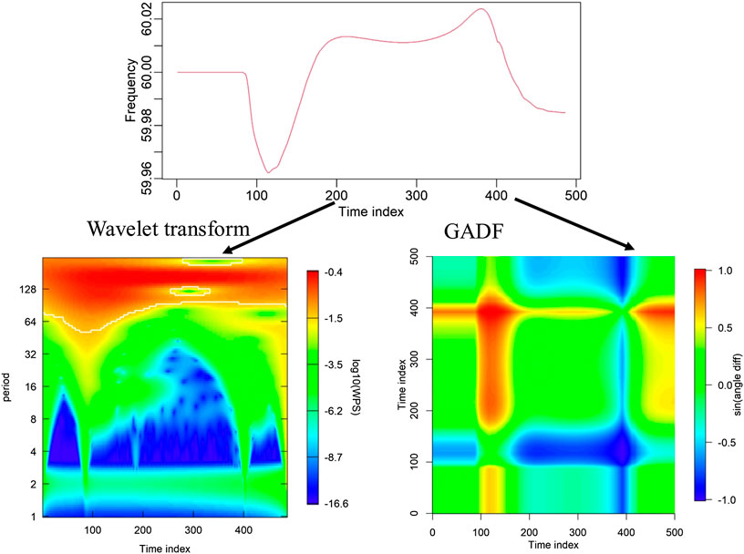
FIGURE 2. A single time series imaged with two different encoding approaches.

CNN Model Development

We designed the CNN architecture to train models for fault type prediction and zonal classification for the Polish 3120-bus system. The inputs to the CNN model training were the image sets produced by three different data encoding schemes, as explained in the methodology section. Model training and testing were done for each data encoding scheme separately and the corresponding model performances were then compared. Each image data set has been divided into three independent subsets: training, validation, and testing. Training and validation contain 85% of the total data which are used during model development to determine the optimized model configuration and hyperparameters. The rest 15% of the data is the testing set for evaluating the final CNN model. The training data also include the multi-class labels data that were determined during the ensemble simulation setup. The multi-class labels are fault types for fault classification, and can be fault locations or zones for training CNN models for approximating fault locations.

CNN Model Architecture

The CNN model architecture conducted in this study is based on VGG11 (Simonyan and Zisserman, 2014), which includes three convolutional blocks containing multiple convolutional layers followed by pooling and dropout layers within each block, and then connected to flatten and dense layers. The detailed model architecture is illustrated in Figure 3 with each block representing one layer. The input to the first 2D convolutional layer is fixed size 128 × 128 RGB image sets. Each image is passed through a series of blocks of convolutional layers (orange layers). A total of three sets of convolutional layers are adopted, which contain 2, 3, and three consecutive convolutional layers, respectively. Different numbers of neural nodes are used for convolutional blocks and the receptive field is consistent for each convolutional layer. Spatial pooling is carried out by three max-pooling layers, following each convolutional block. The function of spatial pooling is to progressively reduce the spatial size of the representation to reduce the number of parameters and computation demand in the network. Max pooling is performed over a 2 × 2-pixel window, with a stride of 2. A dropout layer follows each max-pooling layer. Dropout is a regularization technique that randomly disables a selected fraction of neurons during training to make model performance more robust and prevent overfitting (Hinton et al., 2012). The output from the three blocks of convolutional layers is converted into a 1D feature array by flattening each layer to feed the next layers. Finally, three fully connected layers, also known as dense layers, are added followed by Soft-max activation to yield multi-class predictions. The Soft-max layer outputs values between 0 and 1 to quantify the probability of and confidence in which class each image belongs to. ReLU (i.e., rectified linear unit) activation is one of the most commonly used activation functions in neural networks, especially in CNNs; its output is linear for positive values and zero for negative inputs. In our CNN model architecture, the ReLU activation function is deployed in each layer except the last dense layer. The optimizer is stochastic gradient descent (SGD), which estimates the error gradient for the current state of the model using the training dataset, then updates the weights of the model with backpropagation. The categorical cross-entropy class is chosen for the multi-label classification problems. It computes the cross-entropy loss between the labels and model predictions, and calculation of the loss function requires that the last dense layer is configurated with the total number of classes; this enables Soft-max activation to predict the probability for each class.

FIGURE 3

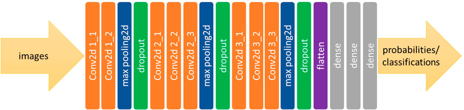
FIGURE 3. The CNN model architecture.

Optimizing CNN Model Configuration

Hyperparameter searching was performed to optimize model configuration during the process of training the CNN model. In our CNN framework, we explore a set of configuration parameters, including learning rate, batch size, kernel size, number of neurons in each convolutional block, and dropout rate. We chose the optimal configuration based on model performance with validation data and then applied it to the testing data set to avoid model bias.

The learning rate is a hyperparameter that controls how much the model changes in response to the estimated error each time the model weights are updated. Choosing the learning rate is challenging, because too small a value may result in a long training process that could get stuck, whereas too large a value may result in learning a suboptimal set of weights too fast or an unstable training process. The batch size is the number of samples in the training set processed before each model updates. The kernel size is the size of the convolutional filter, which is the width × height of the filter mask sliding across every pixel in an image. The next premasters included in the hyperparameter search are the numbers of neurons in each convolutional block. The number of neurons in a convolutional layer is the size of the output of the layer. Each neuron performs a different convolution and provides its own activation for each position. The last parameter tuned in our optimization process is the dropout rate, i.e., the fraction of randomly selected neurons to be disabled. The values chosen for dropout rate were 0.1, 0.3, and 0.5 in the experiments, where a dropout rate of 0.5 leads to the maximum regularization. Because there are multiple tuning parameter types and values, the validation accuracy was estimated for each model configuration combination. Optimization of hyperparameter searching is illustrated in Figure 4 using zonal models as an example. The tuning parameters include the number of neurons in different blocks, kernel size, batch size, dropout rate, and learning rate. In Figure 4, we compare the model accuracy listed as the last axis to the right. Each axis in the figure represents a tuning model parameter and the numbers on each axis are prior selected parameter values. The lines are the combinations of model configurations we tuned in the CNN model. The validation accuracy of each model is color coded to show the optimized model configuration, which can be obtained by tracing back the warm-colored lines for each parameter.

FIGURE 4

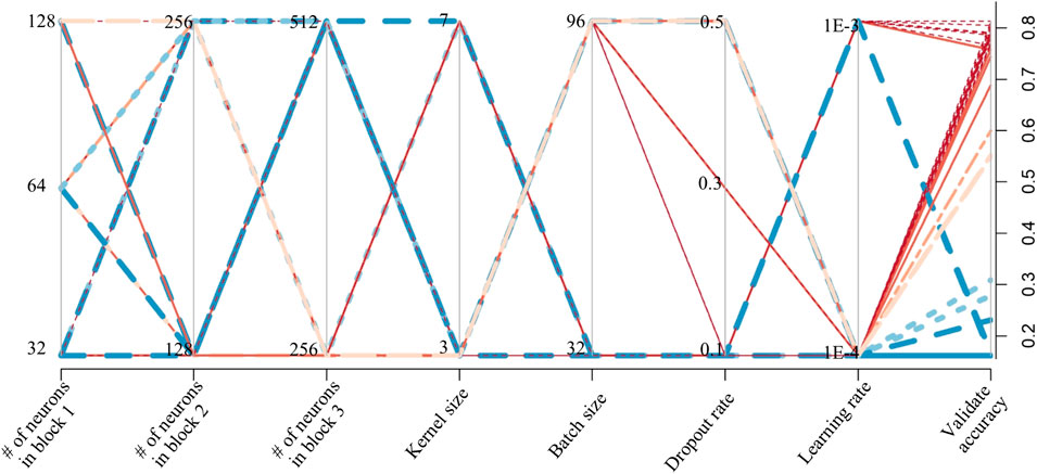
FIGURE 4. Hyperparameter optimization chart. The warm-colored lines represent the model configurations with higher validation accuracy, and the cool-colored lines are the model configurations with lower validation accuracy.

Results and Discussion

To evaluate the CNN model performance with respect to zonal and fault-type classification, a confusion matrix was introduced for multinomial classification. The confusion matrix provides the numbers of the target class values that are assigned to the positive and the negative classes. Four types of events are counted for the multi-class confusion matrix, including 1) True Positive (TP), which is the cells identified by row and column for the positive class that were correctly classified as such. The TP cells are located at the top left corner of the confusion matrix. 2) For False Negative (FN), the row is the positive class and the column is the negative class. FN applies to cells in the positive class that were incorrectly classified as negative, and is located at the top right of the confusion matrix. 3) False Positive (FP) is determined by rows for the negative class and the column for the positive class. FP applies to cells that belong to the negative class that were incorrectly classified as positive, and is placed in the lower left on the confusion matrix; 4) True Negatives (TN) are cells outside the row and column of the positive class. They belong to the negative class and were correctly classified as such. TN is placed at the lower right of the confusion matrix. Using the counts for each of the four types in the confusion matrix, the class statistics metrics, including sensitivity, specificity, precision and accuracy, can be calculated to quantify the model performance. Sensitivity measures how well the model detects events in the positive class. Specificity measures how correct the assignment to the positive class is. Precision measures how good the model is at assigning positive events to positive classes. Accuracy represents the percentage of correctly classified applications out of the total number of applications.

Zonal Classification

The well-trained CNN model using the training and validation data sets was then applied on the third independent testing data set for providing unbiased evaluation of the model. The zonal classification using time-stacked images. The class statistics were calculated and are illustrated in Figure 5. The overall average accuracy metrics among the five zones reached 91% with the straightforward time-series-stacking approach. Zone 1 and Zone 3 had the lowest and highest metrics of accuracy, i.e., 88 and 96%, respectively. The specificity metric was high for all zones, with an average of 97%, which means the model has satisfactory performance in assigning events to the positive class. For sensitivity and precision measurements, both averaged values are about 86%, and Zone 3 stands out among the five zones. All the measured metrics show a high performance level, which means the Polish system has well-defined zonal structures and the CNN model can accurately predict the fault locations.

FIGURE 5

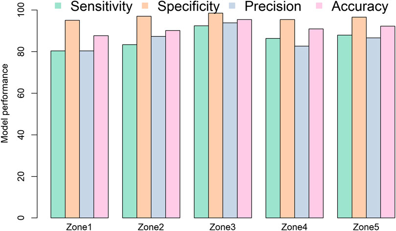
FIGURE 5. Zonal CNN model-performance confusion matrix using a time-domain–stacked encoding approach.

To enable further insight into the model results, the details of class predictions under each targeted class are presented in Figure 6. There were 66 test images for each targeting zone and the bars show the counts of the model predictions each class. In general, the majority of model predictions of the individual classes are correct; i.e., the bar for a given zone (shown in red) has the most counts and the correct classification cases strongly dominate. Generally, a fault added to zones outside the target zone can affect the power flows in the target zones if the zones are physically connected to each other. The physical connections and effects between zones will slightly increase the FT and FN in model predictions. However, if the zones are not connected, the model can provide accurate TN predictions. Zone 1 has the worst prediction results, especially for sensitivity and accuracy, since the model tends to predict a small portion of Zone 1 events as occurring in the other zones, especially Zone 2 and Zone 5. This may be because Zone 1 has connections with all the other zones, which means the flows within Zone 1 are complex and can be affected by the faults attributed to other zones. The largest zone, Zone 3, has no transmission lines going to Zone 5, and our model results showed that none of the predictions for Zone 3 fall in Zone 5. A similar pattern can be seen for the model predictions for Zone 5: no prediction goes to Zones two or three because Zone 5 does not have physical connections with these two zones.

FIGURE 6

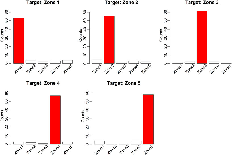
FIGURE 6. Zonal CNN model prediction for each zone using time-domain–stacked encoding approach.

Fault Classification

The class statistics for fault classification using the testing data set using time-stacked images are summarized in Figure 7. Generally, the overall class statistics are lower than those for zonal classification. Quantitatively, the measurement of average fault classification accuracy is 76%. Fault 2 had the highest accuracy, 87%. The prediction accuracy metrics for Fault 1 and Fault 3 are similar, and are around 64%. Specificity metrics were better than the other statistics, thus showing the model’s ability to assign the correct positive classes. The measurement of sensitivity for Fault 4 was lowest at ∼45%, which indicates it is challenging for the current model to detect Fault 4 events and assign them to the positive class. The precision measurements for Faults 1, 3, and 4 are in the range of 55% to 60%. Some of the faults share similar characteristics, which complicates model prediction. For example, both Fault 3 and Fault 4 are generator faults; the difference is that Fault 4 has two neighboring generators out-of-service. The numbers illustrate that model improvements are needed in terms of accurate assignment of positive events to positive classes. The images converted by straightforward time-domain stacking trained in the current CNN model do not contain adequate information for the model to learn the different fault types in the system. More advanced and complex time series for image conversion are adopted to extract more features and pattern characteristics.

FIGURE 7

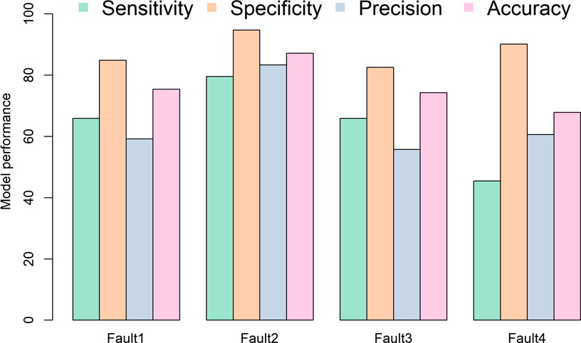
FIGURE 7. Fault type CNN model performance confusion metric using time-domain–stacked encoding approach.

To improve the model performance in fault classification, the frequency-domain and GAF-stacked encoded images were used to retrain the CNN models. Comparisons of model performance using the accuracy metric with different time-series–encoding approaches are shown in Figure 8. Compared with time-domain–stacking method, both frequency-domain–stacking and GAF-stacking approaches increase the accuracy except for Fault 3. The most significant improvement occurs on Fault 1: frequency-domain stacking has 87% accuracy, which is 12% higher than for time-domain stacking. GAF stacking reaches the highest accuracy, 97%, for both Fault 1 and Fault 2; these values are 20% and 10% higher than time-domain–stacking predictions, respectively. For Fault 4, all three encoding approaches have poor performance: the frequency-domain–stacking approach improves the accuracy by 6%, reaching 74%. Meanwhile the GAF stacking accuracy reaches 79%, which is 5% higher than frequency-domain stacking. However, time-domain–stacked encoding works better than the other two advanced encoding approaches for Fault 3.

FIGURE 8

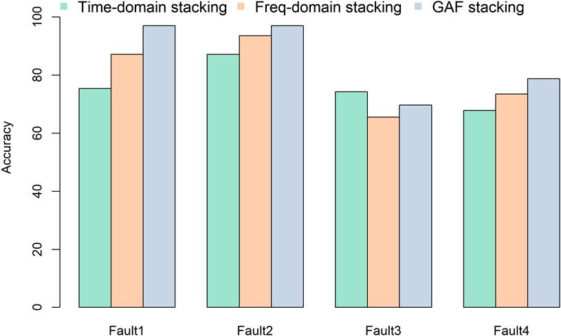
FIGURE 8. Model accuracy results from different encoding approaches.

Detailed class predictions for each targeted class using different encoding approaches are presented in Figure 9. In general, most model predictions of the individual classes are correct for all three encodings except for Fault 3. As the most challenged fault type, time-domain stacking provides limited predictions to Fault 1 and Fault 4 and both frequency-domain stacking and GAF stacking tend to predict Fault 3 to Fault 4. For Fault 4, time-domain stacking has about half predictions for Fault 3 and slightly more predictions for Fault 4. This is because the characteristics of Faults 3 and 4 are similar and both of them are in “outage of generator” category. The model has difficulty distinguishing a single generator fault from a fault of two neighboring generators. However, it is noteworthy that when the target fault is Fault 3 or Fault 4, the model will not provide the predictions to Fault 2. The GAF-stacking based model does not provide any predictions to Fault 1 either. The reason is that Fault 2 is a bus fault whose characteristics are different from the generator faults. Vice versa, when the target fault is fault 2, the model will never provide the predictions to Faults 3 or 4. However, Fault 2 shares some patterns with Fault 1 because a bus fault can affect the transmission lines connected through the buses. For Fault 1, the majority of predictions are in the correct fault category. Both frequency-domain stacking and GAF stacking provide very limited predictions to Fault 2, but the GAF encoding approach provides no predictions to Faults 3 or 4. From the physical perspective of the Polish system, Fault 1 is a single-generator, multiple-line fault, which shares the patterns with all the other three faults because it has faults added on both generator and transmission lines.

FIGURE 9

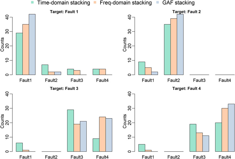
FIGURE 9. Evaluation of CNN model predictions resulting from different encoding approaches.

Conclusion

In this study, we developed and evaluated a deep-learning CNN model to identify locations and predict types of various faults in the Polish 3120-bus system. Four distinct types of faults in different spatial zones and locations were simulated in the Polish system, and the outputs provided adequate and balanced data for CNN training and testing. Our CNN is composed of convolutional, pooling, dropout, and dense layers, which are designed to adaptively learn spatial hierarchies of features. Hyperparameter searches were performed to determine the optimal model configuration and the final model for fault classification and prediction. To enable a powerful, image-based CNN for pattern recognition and extraction, the PMU monitoring time series were encoded in three different ways, including time-domain stacking, frequency-domain stacking and GAF stacking, for generating the image datasets for CNN model training and testing. Different classified responses were benefit from different time-series encoding approaches.

Overall, the line fault and single-bus fault can be classified accurately through fault classification and localization from the PMU monitoring time-series–encoded images with the CNN framework. Different time series encoding techniques can benefit different classified responses. GAF stacking, in particular, when combined with CNN, yields an accuracy around 90% or above for all fault types. The CNN framework was also tested for predicting fault zones or locations, and in general, the fault location is easier to predict than the fault type. For example, using time-domain stacking data, we can achieve 91% accuracy for zonal classification. In practice, both the wavelet decomposition-based frequency-domain stacking and polar coordinate system-based GAF stacking approaches are superior to the time-domain–stacking method, and GAF stacking is recommended to enable deep learning classification to distinguish the fault types that share the similar patterns.

Data Availability Statement

The raw data supporting the conclusions of this article will be made available by the authors, without undue reservation.

Author Contributions

HR contributed to the CNN model implementation, ZH conceived the overall methodologies, BV and PE performed power flow dynamic simulation using PSS/E software and processed the results. HW discussed the results with the team. All authors contributed to writing the manuscript.

Funding

Pacific Northwest National Laboratory is operated by Battelle for the United States Department of Energy under Contract DE-AC05-76RL01830.

Conflict of Interest

The authors declare that the research was conducted in the absence of any commercial or financial relationships that could be construed as a potential conflict of interest.

Acknowledgments

This research was supported by the United States Department of Energy’s Office of Electricity through the Consortium for Electric Reliability Technology Solutions (CERTS).

References

Alhelou, H. H., Golshan, M. H., and Askari-Marnani, J. (2018). Robust sensor fault detection and isolation scheme for interconnected smart power systems in presence of RER and EVs using unknown input observer. Int. J. Electr. Power Energy Syst. 99, 682–694. doi:10.1016/j.ijepes.2018.02.013

PubMed Abstract | CrossRef Full Text | Google Scholar

Avdakovic, S., Nuhanovic, A., Kusljugic, M., and Music, M. (2012). Wavelet transform applications in power system dynamics. Electric Power Systems Research. 83 (1), 237–245. doi:10.1016/j.epsr.2010.11.031

PubMed Abstract | CrossRef Full Text | Google Scholar

Basumallik, S., Ma, R., and Eftekharnejad, S. (2019). Packet-data anomaly detection in PMU-based state estimator using convolutional neural network. Int. J. Electr. Power Energy Syst. 107, 690–702. doi:10.1016/j.ijepes.2018.11.013

PubMed Abstract | CrossRef Full Text | Google Scholar

Canziani, A., Paszke, A., and Culurciello, E. (2016). An analysis of deep neural network models for practical applications. arXiv:1605.07678 [preprint].

PubMed Abstract | Google Scholar

Chen, J., and Patton, R. J. (2012). Robust model-based fault diagnosis for dynamic systems.. Berlin, Germany: Springer Science & Business Media.

Chen, Y. Q., Fink, O., and Sansavini, G. (2017). Combined fault location and classification for power transmission lines fault diagnosis with integrated feature extraction. IEEE Trans. Ind. Electron. 65 (1), 561–569. doi:10.1109/TIE.2017.2721922;

PubMed Abstract | CrossRef Full Text | Google Scholar

Costamagna, P., De Giorgi, A., Magistri, L., Moser, G., Pellaco, L., and Trucco, A. (2015). A classification approach for model-based fault diagnosis in power generation systems based on solid oxide fuel cells. IEEE Trans. Energy Convers. 31 (2), 676–687. doi:10.1109/TEC.2015.2492938

PubMed Abstract | CrossRef Full Text | Google Scholar

Gopakumar, P., Mallikajuna, B., Reddy, M. J. B., and Mohanta, D. K. (2018). Remote monitoring system for real time detection and classification of transmission line faults in a power grid using PMU measurements. Protection and Control of Modern Power Systems. 3 (1), 16. doi:10.1186/s41601-018-0089-x

PubMed Abstract | CrossRef Full Text | Google Scholar

Gopakumar, P., Reddy, M. J. B., and Mohanta, D. K. (2015). Transmission line fault detection and localisation methodology using PMU measurements. IET Gener. Transm. Distrib. 9 (11), 1033–1042. doi:10.1049/iet-gtd.2014.0788

PubMed Abstract | CrossRef Full Text | Google Scholar

Grigsby, L. L. (2016). Power system stability and control. Boca Raton, FL: CRC press.

PubMed Abstract | Google Scholar

Grossmann, A., and Morlet, J. (1984). Decomposition of Hardy functions into square integrable wavelets of constant shape. SIAM J. Math. Anal. 15 (4), 723–736. doi:10.1137/0515056

PubMed Abstract | CrossRef Full Text | Google Scholar

Gu, J., Zhenhua, W., Jason, K., Lianyang, M., Amir, S., Bing, S., et al. (2018). Recent advances in convolutional neural networks. Pattern Recognition. 77, 354–377. doi:10.1016/j.patcog.2017.10.013

PubMed Abstract | CrossRef Full Text | Google Scholar

Guillen, D., Paternina, M. R. A., Zamora, A., Ramirez, J. M., and Idarraga, G. (2015). Detection and classification of faults in transmission lines using the maximum wavelet singular value and Euclidean norm. IET Gener. Transm. Distrib. 9 (15), 2294–2302. doi:10.1049/iet-gtd.2014.1064

PubMed Abstract | CrossRef Full Text | Google Scholar

Han, R., and Zhou, Q. (2016). “Data-driven solutions for power system fault analysis and novelty detection,” in 2016 11th international conference on computer science & education. Nagoya, Japan, August 23–25, 2016, (IEEE), 86–91.

PubMed Abstract | Google Scholar

He, K., Zhang, X., Ren, S., and Sun, J. (2016). “Deep residual learning for image recognition,” in Proceedings of the IEEE conference on computer vision and pattern recognition (CVPR), Las Vegas, NV, June 27–30, 2016, 770–778.

PubMed Abstract | Google Scholar

Hinton, G. E., Srivastava, N., Krizhevsky, A., Sutskever, I., and Salakhutdinov, R. R. (2012). Improving neural networks by preventing co-adaptation of feature detectors. arXiv:1207.0580 [preprint].

PubMed Abstract | Google Scholar

Hochreiter, S., and Schmidhuber, J. (1997). Long short-term memory. Neural Computation. 9 (8), 1735–1780. doi:10.1162/neco.1997.9.8.1735

PubMed Abstract | CrossRef Full Text | Google Scholar

Jan, S. U., Lee, Y.-D., Shin, J., and Koo, I. (2017). Sensor fault classification based on support vector machine and statistical time-domain features. IEEE Access. 5, 8682–8690. doi:10.1109/access.2017.2705644

PubMed Abstract | CrossRef Full Text | Google Scholar

Krizhevsky, A., Sutskever, I., and Hinton, G. E. (2012). Imagenet classification with deep convolutional neural networks. Commun ACM 60, 84–90.

PubMed Abstract | Google Scholar

Livani, H., and Evrenosoğlu, C. Y. (2012). “A fault classification method in power systems using DWT and SVM classifier,” in PES T&D 2012, Orlando, FL, May 7–10, 2012, (IEEE), 1–5.

PubMed Abstract | Google Scholar

Malhotra, P., Vig, L., Shroff, G., and Agarwal, P. (2015). “Long short term memory networks for anomaly detection in time series,” in ESANN 2015 proceedings, European symposium on artificial neural networks, computational intelligence and machine learning, Bruges, Belgium, April 22–24, 2015.

PubMed Abstract | Google Scholar

Mallat, S. G. (1989). A theory for multiresolution signal decomposition: the wavelet representation. IEEE Trans. Pattern Anal. Mach. Intell. 11 (7), 674–693. doi:10.1109/34.192463

MATPOWER (2008). MATPOWER case archive – “Case3120sp.m” – 2008 summer peak Polish Case.

PubMed Abstract | Google Scholar

Patil, D., Naidu, O., Yalla, P., and Hida, S. (2019). “An ensemble machine learning based fault classification method for faults during power swing,” in 2019 IEEE innovative smart grid technologies-asia, Chengdu, China, May 21–24, 2019, (IEEE), 4225–4230.

PubMed Abstract | Google Scholar

Paul, D., and Mohanty, S. K. (2019). “Fault Classification in transmission lines using wavelet and CNN,” in 2019 IEEE 5th international Conference for Convergence in Technology, Bombay, India, March 29–31, 2019, (IEEE), 1–6.

PubMed Abstract | Google Scholar

Qu, N., Li, Z., Zuo, J., and Chen, J. (2020). Fault Detection on insulated overhead conductors based on DWT-LSTM and partial discharge. IEEE Access. 8, 87060–87070. doi:10.1109/ACCESS.2020.2992790

PubMed Abstract | CrossRef Full Text | Google Scholar

Ren, H., Hou, Z., and Etingov, P. (2018a). “Online anomaly detection using machine learning and HPC for power system synchrophasor measurements,” in 2018 IEEE international conference on probabilistic methods applied to power systems, Boise, ID, June 24–28, 2018, (IEEE), 1–5

.PubMed Abstract | Google Scholar

Ren, H., Hou, Z., Wang, H., Zarzhitsky, D., and Etingov, P. (2018b). “Pattern mining and anomaly detection based on power system synchrophasor measurements,” in Proceedings of the annual Hawaii international Conference on system sciences: pacific Northwest National lab (PNNL), Richland, WA.

PubMed Abstract | Google Scholar

Russakovsky, O., Deng, J., Su, H., Krause, J., Satheesh, S., Ma, S., et al. (2015). Imagenet large scale visual recognition challenge. Int. J. Comput. Vis. 115 (3), 211–252. doi:10.1007/s11263-015-0816-y

PubMed Abstract | CrossRef Full Text | Google Scholar

Saleh, S., Moloney, C., and Rahman, M. A. (2008). Implementation of a dynamic voltage restorer system based on discrete wavelet transforms. “IEEE Trans. Power Deliv. 23 (4), 2366–2375. doi:10.1109/tpwrd.2008.2002868

PubMed Abstract | CrossRef Full Text | Google Scholar

Sermanet, P., Eigen, D., Zhang, X., Mathieu, M., Fergus, R., and LeCun, Y. (2013). Overfeat: integrated recognition, localization and detection using convolutional networks. arXiv:1312.6229 [preprint].

PubMed Abstract | Google Scholar

Shorten, C., and Khoshgoftaar, T. M. (2019). A survey on image data augmentation for deep learning. J. Big Data. 6 (1), 60. doi:10.1186/s40537-019-0197-0

PubMed Abstract | CrossRef Full Text | Google Scholar

Simonyan, K., and Zisserman, A. (2014). Very deep convolutional networks for large-scale image recognition. arXiv:1409.1556 [preprint].

PubMed Abstract | Google Scholar

Tan, M., and Le, Q. V. (2019). Efficientnet: rethinking model scaling for convolutional neural networks. arXiv:1905.11946 [preprint].

PubMed Abstract | Google Scholar

Thanaraj, K. P., Parvathavarthini, B., Tanik, U. J., Rajinikanth, V., Kadry, S., and Kamalanand, K. (2020). Implementation of deep neural networks to classify EEG signals using gramian angular summation field for epilepsy diagnosis. arXiv:2003.04534 [preprint].

PubMed Abstract | Google Scholar

Wang, S., Dehghanian, P., and Li, L. (2019). Power grid online surveillance through PMU-embedded convolutional neural networks. IEEE Trans. Ind. Appl. 56 (2), 1146–1155. doi:10.1109/IAS.2019.8912368

PubMed Abstract | CrossRef Full Text | Google Scholar

Wang, Z., and Oates, T. (2015a). “Encoding time series as images for visual inspection and classification using tiled convolutional neural networks,” in Workshops at the twenty-ninth AAAI Conference on artificial intelligence, Vol. 1.

PubMed Abstract | Google Scholar

Wang, Z., and Oates, T. (2015b). “Imaging time-series to improve classification and imputation,” in Twenty-fourth international joint Conference on artificial intelligence.

PubMed Abstract | Google Scholar

Yusuff, A., Jimoh, A., and Munda, J. (2011). Determinant-based feature extraction for fault detection and classification for power transmission lines. IET Gener. Transm. Distrib. 5 (12), 1259–1267. doi:10.1049/iet-gtd.2011.0110

PubMed Abstract | CrossRef Full Text | Google Scholar

Zeiler, M. D., and Fergus, R. (2014). “Visualizing and understanding convolutional networks,” in European conference on computer vision (Springer), 818–833.

PubMed Abstract | Google Scholar

Zhang, G., Si, Y., Wang, D., Yang, W., and Sun, Y. (2019). Automated detection of myocardial infarction using a gramian angular field and principal component analysis network. IEEE Access. 7, 171570–171583. doi:10.1109/access.2019.2955555

PubMed Abstract | CrossRef Full Text | Google Scholar

Zhang, J., Swain, A. K., and Nguang, S. K. (2016). Robust observer-based fault diagnosis for nonlinear systems using MATLAB®. Berlin, Germany: Springer.

PubMed Abstract | Google Scholar

Zhang, S., Wang, Y., Liu, M., and Bao, Z. (2017). Data-based line trip fault prediction in power systems using LSTM networks and SVM. IEEE Access. 6, 7675–7686. doi:10.1109/ACCESS.2017.2785763

PubMed Abstract | CrossRef Full Text | Google Scholar

Zhu, Y., Liu, C., and Sun, K. (2018). “Image embedding of pmu data for deep learning towards transient disturbance classification,” in 2018 IEEE International Conference on Energy Internet (ICEI), Beijing, China, May 21–25, 2018, (IEEE), 169–174.

PubMed Abstract | Google Scholar