 Anqi Xu
 Zhijian Zhang
 Huazhi Zhang1
 Yingfei Ma
94% of researchers rate our articles as excellent or good
Learn more about the work of our research integrity team to safeguard the quality of each article we publish.
Find out more
ORIGINAL RESEARCH article
Front. Energy Res. , 27 November 2020
Sec. Nuclear Energy
Volume 8 - 2020 | https://doi.org/10.3389/fenrg.2020.584750
This article is part of the Research Topic Nuclear Power Plant Equipment Prognostics and Health Management Based on Data-driven methods View all 12 articles
Unlike the current risk monitors, Real-time Online Risk Monitoring and Management Technology is characterized by time-dependent modeling on the state duration of components. Given the real-time plant configuration, it eventually provides the time-dependent risk level and importance measures for operation and maintenance management. This paper focuses on the assessment method of time-dependent importance measures and its risk-informed applications in real-time online risk monitoring and management technology, including Fussell-Vesely (FV), risk achievement worth (RAW), and risk reduction worth (RRW). In this study, the values of component importance have been investigated with a time-dependent risk quantification model, as well as the common cause failure treatment model. Here three options of common cause failure treatment have been developed, assuming that the unavailability of a component could be due to an independent factor (Option 1), a common cause factor (Option 2), or an unconfirmed cause (Option 3). In the special case of “what if a component is out-of-service” of the RAW numerator, a hybrid method for the RAW evaluation is presented resulting in a balanced and reasonable RAW value. A simple case study was demonstrated. The results showed that the absolute values and ranking order of time-dependent importance not only reflected the effect of the cumulative state duration of component on risk, but also comprehensively accounted for all possible situations of component unavailability. Moreover, time-dependent importance measures improved and provided novel insights for online configuration management, 1) ranking SSCs/events/human actions for controlling increased risk and optimizing near–term plans; and 2) exempting or limiting temporary configurations during online operation.
The safety and reliability of nuclear power plants (NPP) depend on the inherent safety of reactor design, as well as the operational safety under different operating conditions. The systems, structures, and components (SSC) of NPP would experience state changes due to random failures, maintenance, or permanent design modifications. And the unavailability of components may increase with operational time, which imposes on the risk level during accident scenarios. Thus, it is a fundamental requirement for online operation and maintenance management to be kept informed of the current risk level and importance measures (IMs) of NPP.
Real-time online risk monitoring and management technology (RORMT) is based on a time-dependent living-PSA model and an updated method of NPP (Zhang et al., 2015b). “Time-dependent” refers to the impact of state duration on the reliability of components. “Configuration” means the alignment of the system, component state, environmental conditions, and NPP scenarios. All of them affect the logical values of events (normal, true, false) or reliability parameters (such as failure rate/failure probability of component, frequency of initiating event (IE)) in the time-dependent living-PSA model, named as “RORM model”.
An integrated platform for nuclear power plant real-time online risk monitoring and management (IRORM) was developed as a generic tool for risk-informed operation, online maintenance, and risk-informed management. It consists of four interactive subsystems. The architecture of IRORM was established as shown in Figure 1.
• The state monitoring and fault diagnostics system(SMF) was developed to online monitor and identify the operational states of systems and equipment with running time. So it identifies the real-time configuration of NPP via access to the digital I&C system in NPP.
• The reliability data online collection, analysis, and storage system (RECAS) (Zubair and Zhang, 2011; Ma and Zhang, 2015) was developed to record state changes and failure times of components. It can automatically update the failure probability of components in time, and provide the reliability parameters to the RORM model. In the long run, it can provide long-term restoration of reliability data for multi-units.
• The living-probabilistic safety assessment (LPSA) system is used for modeling and updating an LPSA model. In case of plant configuration changes or after a fixed period, it can automatically be triggered to update the time-dependent LPSA model in time. After that, a parallel computing engine of IRORM would calculate minimal cut sets (MCS) and risk metrics.
• A real-time online risk monitoring and management system (RORM) is a risk monitor (RM) which is used for displaying and evaluating time-dependent risk measures and other related information.
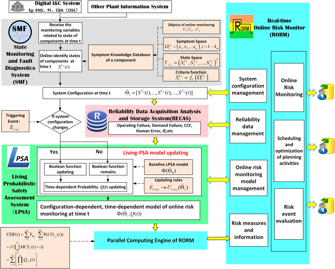
FIGURE 1. Architecture of an integrated platform for nuclear power plant real-time online risk monitoring and management (IRORM).
A variety of IMs were evaluated to identify the risk-significant contributors (Gunnar and Jan, 1994; Kalpesh and Kirtee, 2017) in PRA analysis, for instance, Fussell-Vesely (FV), risk achievement worth (RAW), risk reduction worth (RRW), and Birnbaum importance (Birnbaum, 1969). Among them, FV and RAW have been commonly accepted in engineering practice for SSC categorization (NRC, 2004). The computation of IMs is performed at the level of reliability parameter, individual basic event, event group, as well as component. The IMs of basic events (BE) or components are ranked relatively (Kafka, 1997). In terms of component importance, new measures were introduced to reflect the risk fluctuation due to any events/parameters related to a component, such as the differential importance measure (DIM) (Borgonovo and Apostolakis, 2001), and the component DIM (CPDIM) (Wang et al. 2008). And another treatment for complex components uses a set of minterms (Dutuit and Rauzy, 2015). In the previous literature, several methods for component RAW importance were discussed. For instance, the south Texas project (STP) method (NRC, 2001a) and maximum method (NRC, 2001b) would overestimate the component RAW, while the NEI 00-04 Rev.C method (NEI, 2002) and NEI 00-04 Rev.D method (NEI, 2003) significantly underestimates it. Here three previous methods with respect to the RAW evaluation of components are briefly reviewed including their limitations.
• The “direct method” was used for evaluating RAW directly based on MCSs. For an event group
• To improve the direct method, Check et al. (1998b) suggested that all BE in the event group be replaced with the same indicator, then the Boolean operation was performed to remove the possible non-MCSs. This approach has been widely applied in most risk monitors. However, it only concerned situations when the SSC-related BE can be grouped as one module in fault trees (FT). It also believed that the unavailability of components must be due to independent reasons, and ignored the unavailability situations arising from common cause factors.
• The balancing method (BM) (Kim et al., 2005) considering CCF events was proposed to calculate the RAW importance of components based on Martorell et al. (1996), as expressed in Eq. 1.
Here
But the BM had certain limitations. First, Eq. 1 is derived on the basis that the FV importance of a component is additive. But the basis is insufficient under some circumstances as mentioned in Discussion. Second, the BM is not conservative when the event group of a component consists of more than one basic event. In a word, the methods above were not fully applicable to RORMT.
The time-dependent IMs of components depend on the component lifetime distribution (Borgonovo et al., 2016). They could be evaluated at any time and the ranking order of them may vary with time. To give support for online operation and maintenance, the time-dependent IMs of components should be evaluated and updated in the RORM system whenever the real-time configuration changes. However, some technical challenges still exist in the importance analysis of RORM.
(1) It is necessary to investigate the evaluation method and potential benefits of time-dependent IMs, which is influenced by the time-dependent LPSA model.
(2) It is controversial to extend the importance of a basic event to the level of multiple BE/components (Vaurio, 2011).
(3) It still lacks consensus on updating the CCF model in the case of “what if a component is out-of-service,” such as the numerator of RAW.
In this paper, we agree that both of the independent failure events and CCF events should be considered. Since the unavailability of components is possibly an independent failure, common cause failure, or failure due to an unconfirmed cause, the treatment for unavailability has to balance each assumption. When adjusting the probability of CCF events, it is crucial to account for each unavailability and specific plant configuration.
To solve the problems above, this paper is organized as follows. First, since the time-dependent IMs are affected by both the time-dependent risk and CCF updates, the two mathematical models of risk quantification and CCF treatment are introduced in Mathematical Model of Real-Time Online Risk Monitoring and Management Technology. The time-dependent IMs are presented in Time-Dependent Importance Measures, including FV, RAW, and RRW. The IMs of an individual event are developed to the level of basic event groups/components. A hybrid method for RAW evaluation is proposed by using the three options of CCF treatment in Mathematical Model of Real-Time Online Risk Monitoring and Management Technology. In Case Study, a simple case study is given for demonstration. Time-Dependent Importance Measure for Risk-Informed Decision Making illustrates what the time-dependent IMs contribute to risk-informed decision making, especially for configuration risk management.
The RORM model is a time-dependent LPSA model used for online risk monitoring, which is established by event trees (ET) and FT. Here the concept of time-dependence is explained in Appendix A. Compared with other generic risk monitor models, there are two main enhancements of the RORM model. First, the unavailability of a component changes with its state and running time in the RORM model (as illustrated in Appendix B) while other RMs generally consider the unavailability of components with a fixed mission time or fixed probability. Second, the CCF modeling and updating methods are improved in the RORM model. The CCF updating method on the alpha model (Zubair and Amjad, 2016; Zhang et al., 2017) considered that the failure causes (independent failure, common cause failure, and uncertain cause failure) would influence the reduction of common cause component group (CCCG) order and CCF event probability.
Under any of the following three situations, the RORM model is triggered to update and calculate, according to the modeling and updating rules described (Zhang et al., 2015a; Chen et al., 2020).
(1) Updating due to configuration changes: The structural function
where N is the total number of MCSs (l = 1,2,3,….N).
(2) Regularly updating: The structural function
(3) Reliability parameter updating: The structural function
Assume that: 1) all events (including independent failure events and CCF events) in the RORM model are mutually exclusive, i.e.,
Within the scope of level 1 PRA, the instantaneous risk metric of NPP refers to the core damage frequency (CDF, per unit year). If any possible IE occurs at the current moment t, CDF(t) estimates the frequency of core damage given the real-time plant configuration after a predefined mission time Tm. Based on Eq. 2, the time-dependent risk measure CDF(t) can be quantified using rare event approximation which is mathematically expressed as
where
Note that:
A set of BEs with similar attributes would constitute a BE group, such as BE related to a component, system, or safety function. For instance, a BE group
For an event group
where
Note that the first term refers to the sum of frequencies of MCSs containing any event in the event group. The second term
In this section, three options of what if treatment of unavailability are derived by solving the RORM model with adjusted CCF probability, reflecting the knowledge that a component is out of service. They provide a new idea considering CCF to quantify the what if risk of RAW numerator and RRW denominator.
For an n-order CCCG, the probability of k component failures and total failure probability are expressed in Eqs 6, 7. (1≤k≤n)
where
Option 1: what if unavailability of SSC due to independent factor
The independent factor refers to independent failure, or other preventive maintenance, or tests. When i specific components are identified to be unavailable, the probability of CCF events essentially remains, but they are reorganized to a new CCF event group.
where
Thus, it is required to regenerate CCF events and update their probabilities, without updating CCF parameters in this case.
Option 2: what if unavailability of SSC due to common cause factor
Suppose that a certain common cause factor
From Eq. 9, when a known common cause factor
For i failures of n-order CCCG due to
where
From Eqs 11, 12, the probability of a CCF event due to a common cause factor is higher than that of an independent factor, that is,
Option 3: what if unavailability of SSC due to unconfirmed cause
During the online operation of NPP, it is often impossible to detect the reasons why a component is unavailable (except for some voluntary planned activities such as preventive maintenance and periodic testing). Thus, it is suggested to estimate the probability of CCF events due to unconfirmed causes using the expected value of Option 1 and Option 2.
Given that i components have become unavailable (i = 1, 2, …, n−1), the conditional probability of
where
From Eq. 13, we can obtain the expected probability value of events as Eqs 14, 15.
Based on three basic parameter models for CCF analysis (Mosleh et al., 1998), Option 3 is further developed as follows:
(1) For a β-factor model, if i components are known to have failed, the reason for i failures must be due to an independent factor. So the CCF event probability of the (n-i) remaining components does not change.
(1) For an α-factor model (non-staggered testing scheme):
For an α-factor model (staggered testing scheme):
(1) For an MGL model:
where
For practical considerations, U.S. NRC has proposed methods for CCF treatment. For instance, Appendix E.3 of NUREG/CR-5485(Mosleh et al., 1998) discussed about the condition that one of the components in the CCCG has failed or is under preventive maintenance. But there are two main deficiencies. First, the manner of CCF modeling for a three-order group in the report is “a single common cause basic event (CABC) and three BE (AI, BI, CI)”. This is different from what is currently used in NPP CCF analysis. Second, the approximations of Eqs E.11, E.12 of NUREG/CR-5485 in the report are not valid.
The Risk Assessment of Operational Events handbook (NRC, 2017) had eight CCF treatment cases based on the SAPHIRE software (NRC, 2011). In RASP, given an observed failure of a component in the CCCG, the general consideration is to set the BE of a failed component to TRUE and apply the conditional CCF probability using the original CCF parameter without updating (e.g.,
We have known that the output of RORM might change significantly due to CCF. However, the critical CCF data are hard to obtain. Thus, the following two CCF engineering treatments are applied to the development of IRORM.
• CCF engineering treatment #1: Given a detected random failure of a component
In most cases, it is difficult to quickly determine the failure mode of a failed component online, especially to identify whether it is due to independent failure or CCF. Thus, a tradeoff approach is proposed as follows: for the failed component, set the intermediate event of component “A fails” to be true. For the other components B and C of the same CCCG, the probabilities of certain CCF events (such as CAC, CAB, CABC) are divided by the unavailability Q(t).
• CCF engineering treatment #2: Given preventive maintenance/periodic testing which will lead component A to be unavailable.
In this case, the equipment is unavailable due to independent reasons, but not due to failure. So the basic event “unavailability due to test or maintenance” of A is set to true while the probabilities of CCF events stay the same.
Another possible solution of CCF treatment #2 is to quantify the Boolean function of the RORM model. First, delete all possible BE of component A, and regenerate new CCF trees of comparable components in CCCG. Then update the CCF event probabilities as Option 1 is introduced.
The time-dependent IMs are influenced by the RORM model at time t, but also the CCF treatment, as shown in Figure 2. The importance analysis in PRA is mostly performed based on individual BE or parameters, such as FV (Fussell and Vesely, 1972; Fussell, 1975), RAW, and RRW (Vesely et al. 1986). But for risk-informed applications, the IMs are evaluated to identify the risk-significant SSCs. Thus, in the next section, the time-dependent IMs are defined and evaluated at different levels (basic event, basic event group, and component).
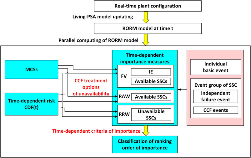
FIGURE 2. The evaluation process of time-dependent importance measures.
The time-dependent FV importance of a basic event
where
For an event group
where
In consideration of engineering practice, FV importance of an individual event which is related to the same component are ranked together, including failure mode events and CCF events. If the FV importance of component C ranks high among components for the current configuration, its preventive maintenance should be preferentially implemented. The operators should be reminded to pay special attention to the components with top FV ranking orders.
The time-dependent
where T is the top event of system failure. Qw(t) is the failure probability of
Note that when calculating
For an event group
where
In consideration of engineering practice,
(1) To avoid certain failures of components:
(2) To prioritize the near-term planned activities of components:
The time-dependent
where
For an event group
where
The RRW importance of unavailable components answers what would happen if it is perfect. Thus, the ranking of RRW can be used to prioritize the maintenance actions.
Since the failure events of unavailable components no longer exist in MCSs, RRW importance of an unavailable component is quantified using MCSs “zero-repair configuration,” in order to find out the missing MCSs. Here “zero-repair configuration” is a virtual configuration with all equipment available, it is predefined by PRA analysts and safety engineers.
The procedures of quantifying
Step 1 Obtain the MCS analysis results of the zero-repair configuration.
Step 2 Except for C, the states of other components are set to their real-time states, in order to generate new MCSs in case component C becomes available again. The logical value of its BE should be consistent with its state, as listed in Table A2 of Appendix B.
Step 3 For component C, its state duration Ts is reset to zero, while the state duration of other components remains unchanged. Update the unavailability of failure events of C.
Step 4 Calculate
Step 5 Determine the RRW of an unavailable component by using the ratio of
If an IM of the union of an event group is the sum of the IMs of the individual BE, then the IM is “additive,” as expressed in Eq. 26.
For a general event group
(1) When
(2) When
(3) In general, if multiple BE are not modeled in a modular FT, there is no certain connection between the FV importance of G and those of individual BE.
It is observed that in the latter two cases, the time-dependent FV importance of G cannot directly sum up the importance of individual BE. Specifically, in most cases, BEs of a component are inputs of OR gate in the RORM model. Thus Eq. 27 is generally used for the FV of a component.
For any of the three situations, neither of the RAW and RRW for an event group are additive, as expressed in Eqs. 30, 31.
The
The treatment of “A component is unavailable” for the numerator of RAW does not mean that “the component does not exist or is removed from the PRA model.” Because “a component is out of service” gives a conditional CCF probability for the remaining components changed according to what type a basic event is. When a component is just out of service with an unconfirmed cause, the component could be out of service due to a common cause factor or due to an independent cause (such as independent random failure, preventive maintenance, or a periodic test).
How to deal with the CCF issue in “what if” is a controversial and tough problem. For a given event group or a component, it should include all related BE and CCF events. But when the logical value of a CCF event is true, it means that two or more components have failed due to a common cause. The probability of other CCF events may become a conditional probability given the known failures in the CCCG. For example, if one of the CCCG elements (such as component C in a three-order CCCG) has been just out of service, the probability of a CCF event which associates C with other components (such as CBC, CAC, and CABC) will increase.
Thus, the reasons for the unavailability of SSC C in CCCG include: 1) a what if independent cause; 2) a common cause factor; and 3) an unconfirmed cause.
Considering the “what if” assumptions of CCF events, a hybrid method to deal with independent failure events and CCF events is proposed to quantify the RAW importance of SSC. The procedures of the hybrid method are shown in Figure 3.
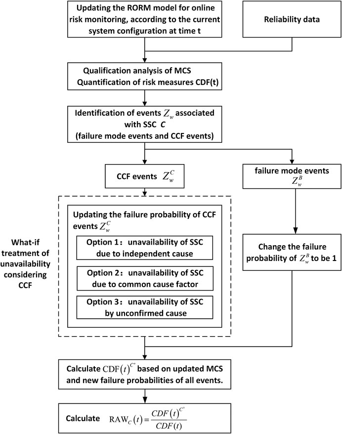
FIGURE 3. Procedures of the RAW importance calculation of SSC C.
Step 1: Update the RORM model according to the real-time plant configuration at time t. The updating rules are concerned with the Boolean function updating of system failure. Qualify the MCSs based on the updated Boolean function of the system.
Step 2The reliability data from the RECAS system are given to quantify the failure probability of failure mode events (refer to Table A2 of Appendix B), CCF events, and IEs, etc. As a result, the risk measures such as CDF(t) are quantified.
Step 3For SSC C, identify all the events
Step 4Update the probability of MCSs under the assumption of “C is out of service.” For CCF events
Step 5Calculate
Step 6The final result
A typical fluid system (Figures 4A) consists of three redundant pump trains. Each train has a 100% pump and its related valve. In normal conditions, at least one pump train of the system supplies water to other systems. P1, P2, and P3 are three redundant and identical electric pumps. The running state of an electrical pump is continuously monitored online, but its standby state cannot be monitored. V1, V2, and V3 are check valves to control the fluid of each pump train. All valves are non-online monitored equipment. When a pump is running/standby, the related valve of the train is open/closed. When the pump is tested/repaired, then the whole pump train (including the related valve) will be out of service for test/maintenance. When the pump happens to fail, the related valve will be automatically triggered to close. The operating pump train normally switches every 30 days-45 days.
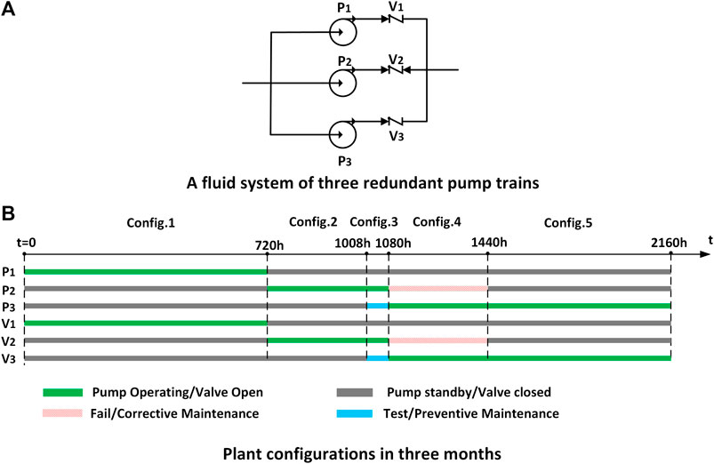
FIGURE 4. Description of fluid system. (A) A fluid system of three redundant pump trains. (B) Plant configurations in three months.
Assumptions and Simplifications:
(1) If the equipment is not online monitored, the last moment to confirm availability is the moment of on-demand action or the end moment of periodic testing/preventive maintenance.
(2) No failure occurs when switching the operating pump train, and no demand failure occurs when a valve transfers its state.
(3) All equipment is available and perfect at t = 0. The pump train #1 is restored to operation. The other two pump trains are in standby.
(4) The mission time of all equipment Tm = 24 h. In this case, the time-dependent risk of the system is a conditional failure probability of the system after the future mission time Tm based on the real-time plant configuration.
(5) The top event of the FT model is “all the pump trains of the system fail to supply water to other systems.”
(6) Only the CCCG of “pump operating failure” is considered in the FT model.
(7) The risk calculation of the system is triggered whenever the configuration changes, and it is regularly calculated every 120 h if the configuration stays the same.
During a 3-month (2,160 h) operation, the system experienced multiple configuration changes as shown in Figures 4B. Train 1 is running, trains 2 and 3 are in standby from t = 0. At t = 720 h, train 1 switches to standby, and train 2 begins to operate. At the same time, V1 becomes closed and V2 becomes open. At t = 1,008 h, the standby pump train 3 starts to carry out a periodic test. At t = 1,080 h, P2 fails randomly. Train 3 changes from standby to operation. Then train 2 enters into online maintenance. At t = 1,440 h, P2 returns to standby, and pump train 3 continues to run.
To demonstrate the time-dependent probabilistic model, the Weibull and exponential distributions of components are used as two examples. If the life distribution of the equipment is exponential, the failure rate is constant. If the life distribution of the equipment follows other continuous distributions such as Weibull distribution, the failure rate varies with time. The reliability parameters of the two examples are listed in Table 1A.
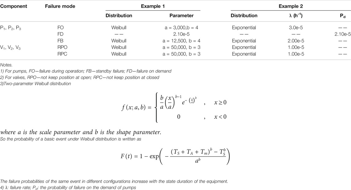
TABLE 1A. Reliability parameters of failure events.
The insights of risk are inaccurate in current RMs. First, PRA data used by RMs are based on the assumption that the “time to failure” of continuous operating equipment is exponentially distributed, that is, the estimated value of failure rate λ(t) is constant. Second, for a predefined mission time of the system, the risk level is only dependent on the plant configuration regardless of state duration, so the risk is constant under the same configuration. From the black lines of Figures 5A, B, we found out that no matter what distribution the life of equipment is, the risk levels of different configurations are almost the same as long as the combination of available equipment is the same, such as Config.1, Config.2, and Config.5. Based on the above risk information of RM, we can infer that the operating equipment is allowed to operate continuously, with no requirements of periodic testing/preventive maintenance or regularly switching between redundant units. That is obviously in contrast with the engineering experience of NPP.
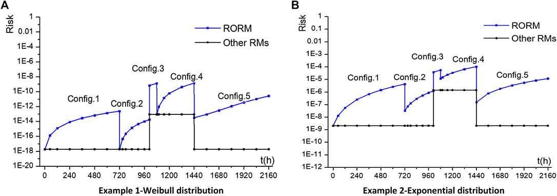
FIGURE 5. Comparison of risk profile between RORM and other RMs. (A) Example 1-Weibull distribution. (B) Example 2-Exponential distribution.
The system risk of RORM varies with plant configuration and equipment unavailability. It is a sort of saw-tooth type. Take the blue line of Figures 5A as an example. For Config.1 (train 1 is running, train 2 and 3 are standby), the risk rises rapidly from baseline risk 1.860e-18 to 2.430e-13. At t = 720 h, train 1 switches to standby, and train 2 begins to operate. At the same time V1 turns to closed and V2 turns to open. For configuration 2, firstly the risk drops to 2.019e-18, which is quite close to the baseline risk, then it increases to 1.751e-14. At t = 1,008 h, the standby pump train 3 starts to carry out a periodic test. For Config.3, the redundancy of the system is reduced, so the risk suddenly increases to 6.794e-10. During the test, the risk rises until the end of test. After the test of train 3, the state durations of P3 and V3 are both reset. At t = 1,080 h, P2 fails randomly. The standby train 3 is put into operation. Then train 2 enters into online maintenance. After the maintenance of train 2, the state durations of P2 and V2 are both reset. For Config.4, the risk drops to 8.954e-14 due to P2 failure, then it increases to 1.3980e-9 with the continuous operation of train 3. At t = 1,440 h, P2 returns to standby, and train 3 continues to run. For Config.5, the risk steps down to 3.1510e-14, and then gradually climbs to 2.633e-11.
The RORM model brings novel risk insights based on the effect of cumulative state duration. Even if the plant configuration remains, the risk also increases with the system running time. By comparison of Config.1, 2, and 5, it is clear that even if the combination of available equipment is the same, the risk levels of different configurations vary from each other. Thus, it is necessary to carry out periodic testing, inspection, maintenance, and switching regularly in order to keep the risk level within an acceptable range.
As mentioned in Time-Dependent Fussell-Vesely Importance, the FV importance values of equipment for Config.1 and 2 are calculated according to the parameters in Example 1, as shown in Figure 6. We can see that the characteristics of time-dependence greatly affect the absolute value of FV. More importantly, the relative rankings of them also change with time. Note that in Config.1, FVP2(t) = FVP3 (t),FVV2 (t) = FVV3 (t).
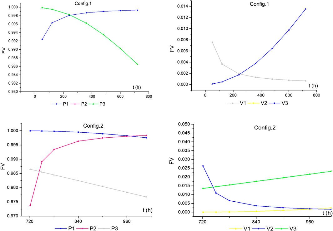
FIGURE 6. FV importance of component (Config.1 and 2).
For the RRW calculation, since the components in the same pump train are in series, the RRW values of these unavailable components are equal. For instance, RRW(P3) = RRW(V3)≈1 for the Config.3.
Example 1 (Weibull distribution) is used in this section for the validation of CCF treatment options. The BE P1-FO, P2-FO, and P3-FO make up a CCCG (CCCG3_FO). The size of CCCG n = 3 with common cause factors l = 2. Table 1B gives the parameters of CCCG at several different time points. The total failure probability
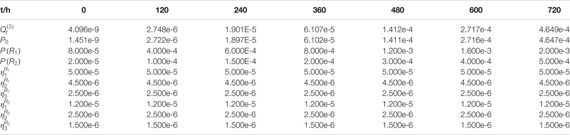
TABLE 1B. Parameters of CCCG (P1-FO,P2-FO,P3-FO).
Note that the CCF model and parameters in the current PRA model are based on statistical failure data and symmetrical assumptions. But in the RORM model, the failure probabilities of three components in the CCCG would be asymmetrical due to different state duration. In this case, to simplify CCF consideration,
The coupling mechanism in CCCG might be location-related, operational-related, maintenance-related, and manufacturer-related, etc. The CCF coupling factors
If A, B, and C are BE P1-FO, P2-FO, and P3-FO respectively, the probability of failure event is expressed as
where
The results of three CCF treatment options are shown in Table 2 if one of components in CCCG is unavailable (i = 1) at t = 120 h. As for the updated probabilities of CCF events in CCCG, Option 2 and Option 3 are greatly larger than those of Option 1, because the conditional probability of a CCF event would rise due to the occurrence of a common cause factor. So it is proven that the engineering practice of Option 1 is not conservative.
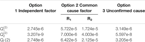
TABLE 2. Results of three CCF treatment options if a component is unavailable (i = 1, t = 120 h).
In RORMT, the numerator of the RAW importance of a component is mainly influenced by what if treatment considering CCF. That is different from other risk monitors. The results of different methods are compared in Tables 3A–C at different time points. Here NUREG/CR-5485 refers to Appendix E3.1 without approximation in this report. RASP refers to the CCF treatment case 1 (when observed failure with the loss of function of one component in the CCCG). By comparing the results in Tables 3A–C, it can be seen that:
(1) For components out of CCCG, RAWs of all methods are almost the same. But for a component in the CCCG, RAW importance values of different methods vary greatly. The direct method only treats with the failure mode events of the component, whose result is not accurate as discussed in PRA Importance Measures and Challenges of Real-Time Online Risk Monitoring and Management Technology. The other methods consider both CCF events and failure mode events.
(2) If a basic event of a component is within a CCCG, such as P1-FO, P2-FO, and P3-FO, the RAW values of that component calculated by the BM and the NUREG/CR-5485 method, are at least two orders of magnitude higher than the other methods. The RAW result obtained by NUREG/CR-5485 is very large, because it does not distinguish the failure cause of the component. The probabilities of all CCF events in CCCG are divided by the total failure probability of the component. And the basic event probability (such as P2-FB) is set to 1. Thus, the components within CCCG are always at the top of the RAW ranking list. However, these results may mislead the operator actions.
(3) Since the CCF treatment of the RASP method and Option 1 are similar, the RAW results of the two methods are quite similar. They both set the failure mode basic event of that component to TRUE and adjust the CCF event probability. The difference is that RASP updates the CCF parameters based on the reduced size of the CCCG, while Option 1 updates the CCF event probability by grouping the time-dependent events into a new CCCG.
(5) For Option 2, the conditional probability of CCF events given a specified common cause factor contributes to the high RAW value. Option 3 in the hybrid method results in the expected value of Option 1 and Option 2. Besides, it is difficult to identify the real cause of failure (independent cause or common cause) as soon as failure happens. It requires more maintenance and inspection work to detect the failure cause. Thus, Option 3 makes sense for online applications of RORMT.
(6) Comparing the results at different times in Config.1, it is found that the absolute values and ranking order of component RAW would change with time for a certain configuration.
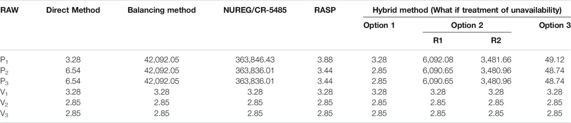
TABLE 3A. RAW importance results of different methods (t = 120 h).
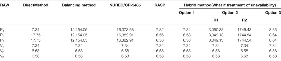
TABLE 3B. RAW importance results of different methods (t = 360 h).
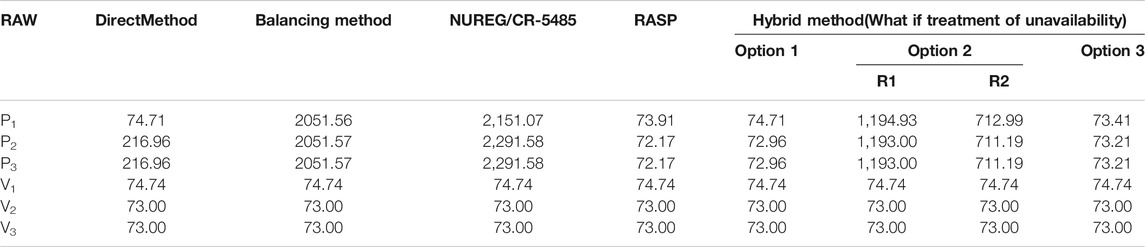
TABLE 3C. RAW importance results of different methods (t = 720 h).
Based on the current plant configuration, the time-dependent IMs of RORM would provide risk insights in the following three groups of activities: 1) ranking SSC activities and human actions for prioritizing maintenance or tests and 2) exempting or limiting temporary configurations beyond limiting conditions for operation (LCOs) of technical specification (TS) with allowed configuration times.
The current risk-informed SSC categorization method for NPP was proposed in 10CFR 50.69 (NRC, 2004). The screening criteria of risk significant SSCs are FV and RAW importance of components based on the average PRA model of NPP. The average PRA model is established in a predefined condition which usually assumes all equipment is in an available state.
However, the 10CFR 50.69 method is offline and static, and not appropriate for SSC importance evaluation in the RORM model. First, the 10CFR50.69 method would not support when some SSCs are out of service. Second, the risk IMs, and risk significance in RORM are strongly dependent on the scenario conditions of NPP, real-time operational state, and state duration of a component. The same equipment will have different importance values under different plant configurations.
To better utilize the ranking order of IMs for online operation, we derive a type of time-dependent criteria of SSC importance from the operational safety criteria (OSC) of NPP. The classification of the instantaneous risk adopted by OSC is usually three-zone or four-zone. Take the three zones (unacceptable risk, high risk, and low risk) of CDF for example. The risk thresholds of CDF are predetermined by a nuclear safety supervisory authority, i.e., threshold between low and high risk (
The threshold of FV, denoted as
where s is the number of risk zones.
Figures 7A indicates the time-dependent criteria of
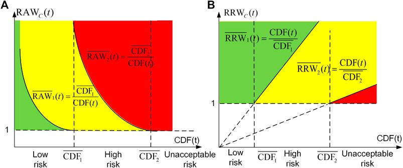
FIGURE 7. Time-dependent criteria of SSC importance. (A) RAW. (B) RRW
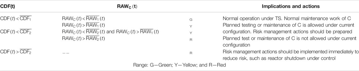
TABLE 4A. Implications and actions of time-dependent criteria of
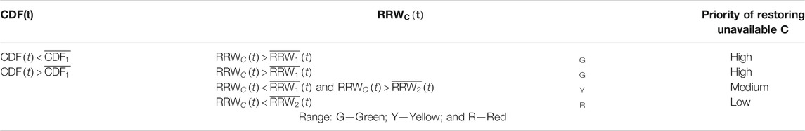
TABLE 4B. Implications and actions of time-dependent criteria of
Although the concepts “risk significance” and “safety significance” are often conflated in risk-informed applications, FV importance is generally regarded as a measure of risk significance, while RAW is that of safety significance (Cheok et al, 1998a; Cheok et al 1998b; NRC, 2019). But they are evaluated based on an average PRA model over different configurations and diverse accident sequences (Vesely, 1998). Youngblood clarified the two concepts and proposed a different measure: the “prevention worth” (Youngblood, 2001) of safety significance. The prevention worth was used in top event prevention analysis (Youngblood and Worrell, 1995; Blanchard et al. 2005).
Online risk evaluation requires quantifying the RORM model given a specific configuration change, or given planned sequential configuration changes. This action is to determine whether planned or temporary plant reconfigurations are sufficiently safe, especially when a planned configuration is overlapped with several unplanned events. In this case, the calculation of risk is mainly affected by time-dependent unavailability and CCF consideration.
Since temporary or emergency events might occur in the real-time configuration, it is necessary to consider the operational configuration changes and provide configuration-specific risk insights by the relative rankings of IMs, such as identifying risk-significant SSC/accident sequences/IEs/human actions. The relative rankings of IMs are utilized as shown in Table 5. In addition, other IMs such as Birnbaum importance (Birnbaum, 1969) and critical importance (Lambert, 1975) could also be evaluated based on real-time plant configuration and state duration.
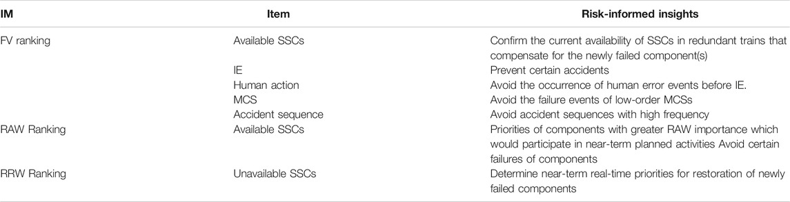
TABLE 5. Risk-informed insights for online operation and maintenance using relative rankings of IMs.
It is worth noting that the uncertainty of relative ranking order of importance (Modarres and Agarwal, 1996; Aven and Nokland, 2010) would be affected by three main factors 1) the distribution of reliability data used, 2) the scope and quality of the RORM model, and 3) the truncation limit of risk calculation.
For maintenance plan scheduling and plan risk assessment, the time-dependent risk measures are also utilized in the real-time online risk monitoring and management method (Xu et al. 2018). If the calculated instantaneous risk or the cumulative risk for a planned sequence of configuration changes is unacceptable, equipment outages should be shortened and re-arranged. Also, the ranking order of IMs of SSCs is used to prepare risk management actions beforehand, so to strictly control the outage duration of equipment maintenance, protecting other risk-significant equipment, and administration control, etc.
RORMT is characterized by time-dependent modeling and updating for online risk monitoring of NPP. It is dependent on the real-time plant configuration and state duration of equipment. This paper discussed the risk-informed assessment and application of time-dependent IMs in RORMT. The time-dependent FV, RAW, and RRW defined for individual BE and event groups of a component. They are not only influenced by the time-dependent risk, but also the CCF treatment. Since the RAW of a component is particularly affected by updating the CCF model in the case “what if a component is out of service,” three CCF treatment options for component unavailability are assumed: 1) Option 1 - independent cause; 2) Option 2 - common cause factor; 3) Option 3 - unconfirmed cause. The updating of CCF order and CCF event probability are discussed for the three options. Accordingly, a hybrid method for RAW evaluation has been proposed based on the three options. Using the hybrid method not only comprehensively accounts for all possible unavailable causes, but also reduces the conventional misunderstanding of component importance. A simple case study is demonstrated through examples of exponential distribution and Weibull distribution.
From the case study, it is found that since the time-dependent risk of the same configuration would increase with the state duration of the equipment, the absolute values and relative rankings of IMs may vary with time. Thus, if the real-time configuration changes or the state duration of a component increases, it is necessary to re-quantify the time-dependent IMs. Moreover, for the updated probabilities of CCF events in CCCG, the results of Option 2 and Option 3 are much larger than those of Option 1. The hybrid method with Option 3 generates a reasonable value for component RAW, and it is more suitable for RORMT.
The time-dependent IMs considering state duration and CCF would provide novel insights for online configuration risk management: 1) ranking SSCs/events/human actions for controlling the increased risk and optimizing near–term plans and 2) exempting or limiting temporary configurations beyond technical specifications with allowed configuration times. Besides, the time-dependent criteria of SSC IMs are established in this paper to further classify the ranking order of RAW and RRW. For practical engineering applications of the proposed methods, the future research will focus on: 1) verifying the time-dependent LPSA modeling with long-term operating data and 2) further study on the CCF failure mechanism to obtain the critical CCF data.
All datasets presented in this study are included in the article/supplementary material.
ZZ instructed and proposed the methodology of the RORM technology. AX conceptualized and implemented this study, and wrote the original draft. HZ dedicated his time to the development of the IRORM program, and validated the method. HW was the project administrator and provided the required resources. MZ provided the basic information about common cause failure modeling. SC and YM assisted in the conceptualization, investigation, and data curation. XD reviewed and verified the results.
This research is currently funded by the National Key R&D Program of China“ titled “Research on Real-time Risk Monitoring, Evaluation and Management Technology of Nuclear Power Plant” (grant no. 2019YFB1900803). Besides, the earlier study was supported by Harbin Engineering University, the National Science and Technology Major Project of China titled “Research on Living PSA and On-line Risk Monitor and Management of Nuclear Power Plant” (grant no. 2014ZX06004-003), and the National High-tech R&D Program of China titled “Research on Online Risk Monitor and Management of Nuclear Power Plant” (grant no. 2012AA050904).
Author MZ was employed by China Nuclear Power Engineering Co., LTD.
The remaining authors declare that the research was conducted in the absence of any commercial or financial relationships that could be construed as a potential conflict of interest.
The authors express gratitude to our former teammates, Wang Yan, Deng Yunli, Li Songfa, and Guo Biao. Besides, the whole team would give thanks to the Beijing Appsoft (Shen Zhou Pu Hui) Technology Co., Ltd. and the Shanghai Yaspeed Information Technology Co., Ltd. for their dedication.
During the online operation of NPP, the plant configuration changes because of random failures of a component, switching between running and standby trains, environment changes, and other activities such as repair work, periodic testing, inspection, and planned maintenance.
In RORMT, the state of equipment (such as valve open and closed, electric pump operation and standby) is either identified as “known” by the state monitoring and fault diagnostics system timely, or manually set by the operational maintenance personnel (after a possible time delay).
Let the state of a component at time t be
The failure of a component in FT is often represented by multiple BE (also called failure events). The failure modes of equipment are defined in different manners among nuclear power units. In order to establish a generalized modeling method and updating rules, the specific failure modes of equipment are roughly grouped into three generalized failure mode categories, i.e., failure on demand (FD), standby failure (SB), and failure during operation (FO), as illustrated in Table A1.
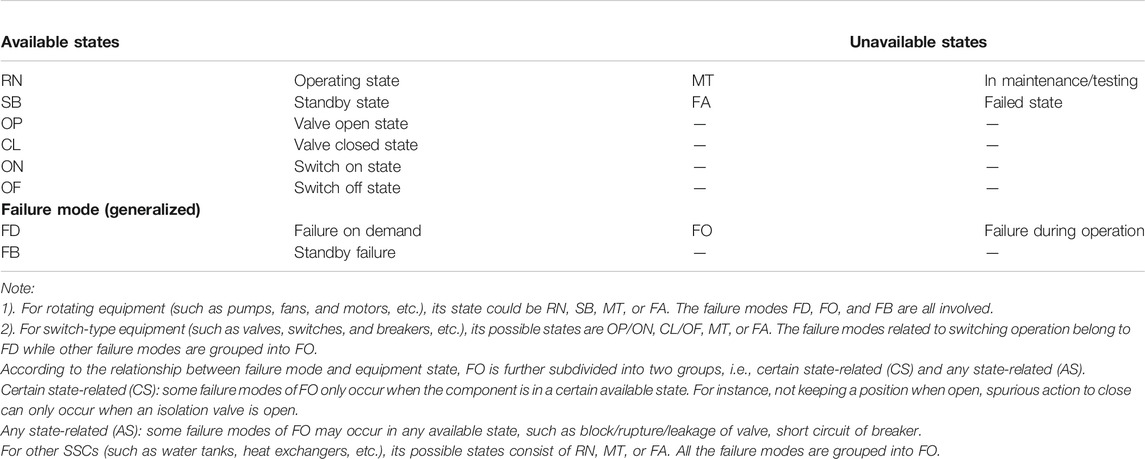
Table A1. Classification of equipment state and failure events in RORMT.
To better illustrate time-dependent unavailability in RORMT, the concept of time-dependence is introduced as shown in the timeline plot of Figure A1. Here time-dependence refers to the real-time state duration of SSC, which is denoted as Ts.
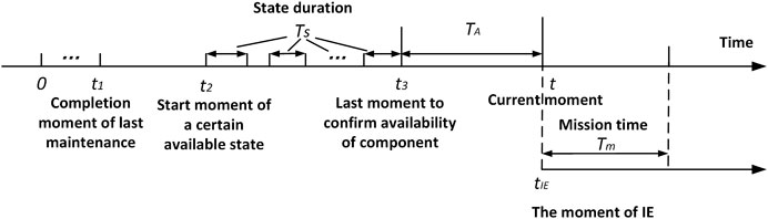
FIGURE A1. Schematic diagram of time-dependent concept.
t: the moment of risk for calculation. For real-time online risk monitoring, t is the current moment.
t1: the completion moment of the last corrective/preventive maintenance of a component.
t2: the moment when a particular available state of a component first appeared after t1. For real-time online risk monitoring, t2 refers to the real-time state of a component.
t3: the last moment to confirm that the component is in an available state after t1. Particularly, for continually monitored components, their states are transferred by sensors or the monitoring unit of the components to RORM at a very high frequency, so t3 and t can be regarded as the same moment for the calculation, t3≈t. For unmonitored components, there is a time delay between t3 and t, since t3 is manually recorded by the last periodic test, on-site inspection, etc.
TA: the period when the availability of the real-time state is not fully confirmed. TA = t-t3. For the continually monitored components, TA≈0. For other unmonitored components, TA is not longer than a test/maintenance period.
tIE: assuming moment when IE occurs. tIE=t.
Ts: the real-time state duration. It is the cumulative time interval of a specific state during the period from t1 to t3. Note that some components may experience multiple state transitions, thus Ts≤(t3-t2).
The assumptions of the RORM model are as follows:
• When a component is in any available state, the real-time state at the current time t is the same as that of t3. Its unavailability is time-dependent on state duration.
• When a component is in any unavailable state, conservatively, its unavailability is assumed to be 1.
• The occurrence time of any IE in the RORM model is assumed at the current moment, tIE=t.
• The failure events of a component in a certain state are mutually independent. The failure events of the same component in different operating states are also independent.
• For the online repairable equipment, the completion of repair and recovery operation can be immediately reported. For the equipment which cannot be repaired online, it must be repaired during the refueling overhaul.
• No maintenance will be continued or carried out after IE.
• If the unavailable equipment has not been recovered and is not in service at the current moment, then it cannot be used for accident mitigation after IE occurs.
• The component/system can be considered “as good as new” after the completion of maintenance or testing. To put it simply, the reliability of equipment is 1.
• The state duration Ts is updated depending on its previous operating history.
The time-dependent probability of a basic event of a component at the current moment
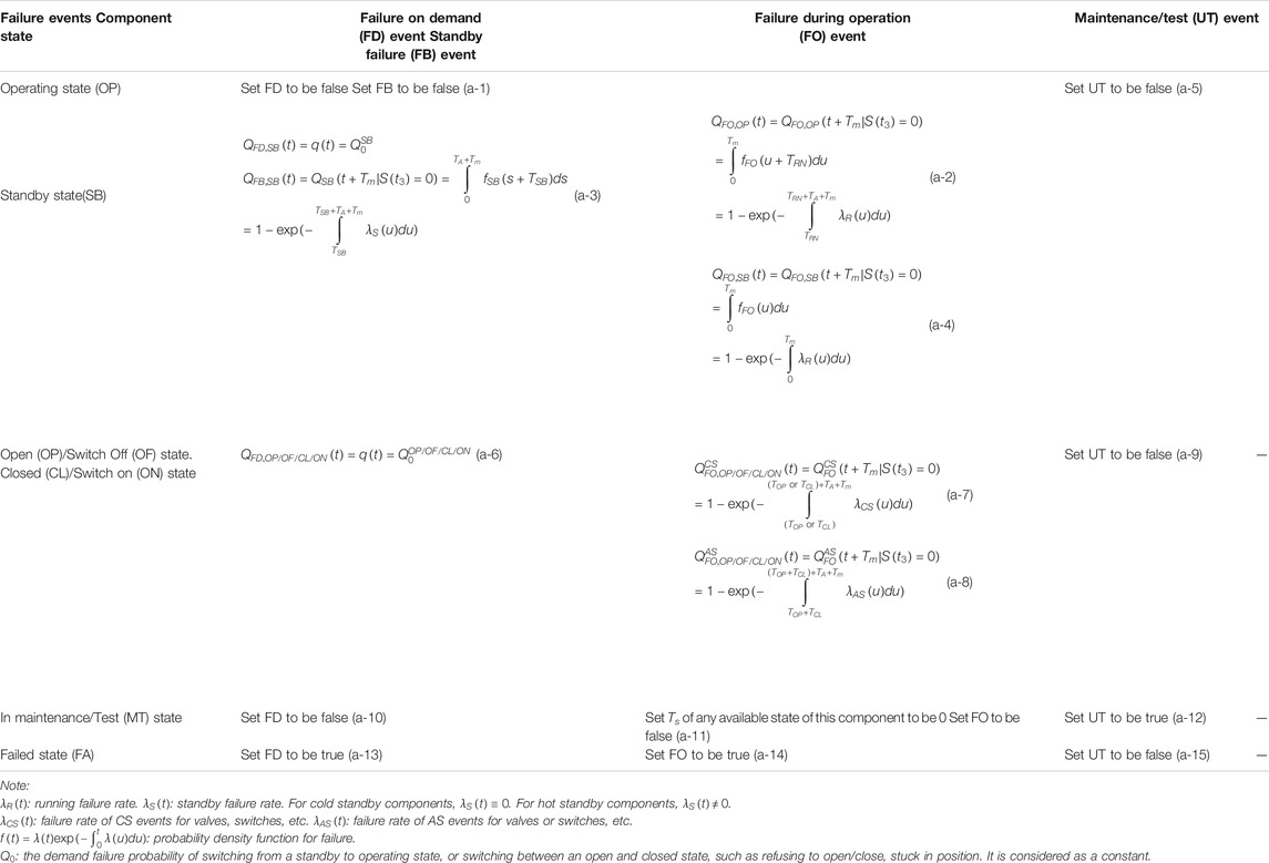
TABLE A2. Time-dependent probability of failure events in the RORM model.
Atwood, C. L., LaChance, J. L., Martz, H. F., Anderson, D. L., Englehardte, M., Whitehead, D., and Wheeler, T. (2003). Handbook of parameter estimation for probabilistic risk assessment. Rockville, MD: Nuclear Regulatory Commission, NUREG/CR-6823.
Aven, T., and Nokland, T. E. (2010). On the use of uncertainty importance measures in reliability and risk analysis. Reliab. Eng. Syst. Safety., 95, 127–133. doi:10.1016/j.ress.2009.09.002
Birnbaum, Z. W. (1969). On the importance of different components in a multi-component system. New York, US: Academic Press, 581–592.
Blanchard, D., Worrell, R. B., and Varnado, B. (2005). Risk-informed physical security; dynamic allocation of resources. in Proceeding of the ANS International Topical meeting on Probabilistic Safety Analysis (PSA 2005). San Francisco: American Nuclear Society.
Borgonovo, E., Aliee, H., Glaßb, M., and Teich, J. (2016). A new time-independent reliability importance measure. Eur. J. Oper. Res. 254, 427–442. doi:10.1016/j.ejor.2016.03.054
Borgonovo, E., and Apostolakis, G. E. (2001). A new Importance measure for risk-informed decision making. Reliab. Eng. Syst. Safety. 72, 193–212. doi:10.1016/s0951-8320(00)00108-3
Chen, S. J., Zhang, Z. J., Zhang, H. Z., Zhang, M., Wang, H., Ma, Y. F., et al. (2020). Research on living PSA method based on time-dependent MFT for real-time online risk monitoring. Ann. Nucl. Energy. 143, 107406. doi:10.1016/j.anucene.2020.107406
Cheok, M. C., Parry, G. W., and Sherry, R. R. (1998a). Response to 'Supplemental viewpoints on the use of importance measures in risk-informed regulatory applications'. Reliab. Eng. Syst. Safety. 60, 261. doi:10.1016/s0951-8320(97)00146-4
Cheok, M. C., Parry, G. W., and Sherry, R. R. (1998b). Use of importance measures in risk-informed regulatory applications. Reliab. Eng. Syst. Safety. 60, 213–226. doi:10.1016/s0951-8320(97)00144-0
Dutuit, Y., and Rauzy, A. (2015). On the extension of importance measures to complex components. Reliab. Eng. Syst. Saf. 142, 161–168. doi:10.1016/j.ress.2015.04.016
Fussell, J. B. (1975). How to hand-calculate system reliability and safety characteristics. IEEE T. Reliab. 24, 169–174. doi:10.1109/tr.1975.5215142
Fussell, J. B., and Vesely, W. E. (1972). A new methodology for obtaining cut sets for fault trees. Trans. Am. Nucl. Soc. 15, 262–263.
Gunnar, J., and Jan, H. (Editors) (1994). Safety evaluation by living probabilistic safety assessment. Procedures and applications for planning of operational activities and analysis of operating experience. Stockholm, Sweden: Swedish Nuclear Power Inspectorate, SKI Technical Report 94: No. NKS/SIK 1, 16.
Kafka, P. (1997). Living PSA-risk monitoring—current use and developments. Nucl. Eng. Des. 175, 197–204. doi:10.1016/s0029-5493(97)00037-x
Kalpesh, P. A., and Kirtee, K. K. (2017). An overview of various importance measures of reliability system. Inter. J.Math., Eng.Management Sci. 2, 150–171. doi:10.33889/IJMEMS.2017.2.3-014
Kim, K., Kang, D. I., and Yang, J. E. (2005). On the use of the balancing for calculation component RAW involving CCFs in SSC categorization. Reliab. Eng. Syst. Safety. 87, 233–242. doi:10.1016/j.ress.2004.04.017
Kuo, W., and Zhu, X. Y. (2012). Importance measures in reliability risk and optimization: principles and applications. New York, U.S.: John Wiley & Sons.
Lambert, H. E. (1975). “Measure of importance of events and cut sets in fault trees,” in Proceedings of conference on reliability and fault tree analysis. Editors Barlow, R.E., Fussell, J.B., and Singpurwalla, N. D. (Philadelphia, PA: Society for Industrial and Applied Mathematics), 77–100.
Ma, Y. F., and Zhang, Z. J. (2015). Development of reliability data analysis system in nuclear power plant. Int. J. Nucl. Safety and Simul. 6, 30–36.
Martorell, S., Serrade, V., and Verdu, G. (1996). Safety-related equipment prioritization for reliability centered maintenance purposes based on a plant specific level I PSA. Reliab. Eng. Syst. Safety. 27, 35–44. doi:10.1016/0951-8320(95)00122-0
Modarres, M., and Agarwal, M. (1996). “Consideration of probabilistic uncertainty in risk-based importance ranking,” in Proceeding of international topical meeting on probabilistic safety assessment. Park City, UT, September 29–3 October, 1996 (La Grange Park, IL: American Nuclear Society).
Mosleh, A ., Rasmuson, D. M., and Marshall, F. M. (1998). Guidelines on modeling common-cause failures in probabilistic risk assessment. Washington, DC: Safety Programs Division, Office for Analysis and Evaluation of Operational Data, U.S. Nuclear Regulatory Commission, Vol. 5485.
NEI (2011). Industry guideline for monitoring the effectiveness of maintenance at Nuclear power plants. NUMARC 93-01 Revision 4A.
NEI (2006). Risk-informed technical specifications initiative 4b. Risk-managed technical specifications (RMTS) guidelines. NEI 06-09(Revision 0)-A
NRC (2004). Risk-informed categorization and treatment of structures, systems and components for nuclear power reactors. 10CFR50.69.
NRC (2019). NRC glossary. Available at: https://www.nrc.gov/reading-rm/basic-ref/glossary/full-text.html (Accessed March 11, 2020)
NRC (2001a). STP nuclear operating company exemption requests: proof-of-concept for risk informed 10 CFR Part 50 Option 2, safety evaluation. SECY-01-0103.
NRC (2001b). Official transcript of proceedings of ACRS plant operations and PRA subcommittee., South Texas Project Exemption Requests.
NRC (2011). Systems analysis programs for hands-on integrated reliability evaluations (SAPHIRE) version 8. NUREG/CR-7039 Vol.2.
Vaurio, J. K. (2011). Importance measures in risk-informed decision making: ranking, optimisation and configuration control. Reliab. Eng. Syst. Safety. 96, 1426–1436. doi:10.1016/j.ress.2011.06.012
Vesely, W. E., Davis, T. C., Denning, R. S., and Saltos, N. (1986). Measures of risk importance and their applications. NUREG/CR-3385.
Vesely, W. E. (1998). Supplemental viewpoints on the use of importance measures in risk-informed regulatory applications. Reliab. Eng. Syst. Safety. 60, 257–259. doi:10.1016/s0951-8320(97)00145-2
Wang et al. (2008). FDS team. Study on the algorithm of the calculation of the components’ importance measures in a risk monitor. Chinese Journal of Nuclear Science and Engineering. 28, 61–65. doi:10.3321/j.issn:0258-0918.2008.01.012
Xu, A. Q., Zhang, Z. J., Zhang, H. Z., Zhang, M., Wang, H., Ma, Y. F., and Chen, et al. (2018). “Real-time online risk monitoring and management method for maintenance optimization in nuclear power plant,” in Proceedings of the 2018 26th international conference on nuclear engineering (ICONE 26). London, UK: American Society of Mechanical Engineers.
Youngblood, R. W. (2001). Risk significance and safety significance. Reliab. Eng. Syst. Saf. 73, 121–136. doi:10.1016/s0951-8320(01)00056-4
Youngblood, R. W., and Worrell, R. B. (1995). “Top event prevention in complex systems,” in Proceedings of the 1995 joint ASME/JSME pressure vessels and piping conference. PVP-Vol. 296, SERA-Vol.3. Honolulu, Hawaii: American Society of Mechanical Engineers.
Zhang, M., Zhang, Z. J., Chen, S. J., and Zhang, H. Z. (2015a). Living PSA modeling and updating for online risk monitoring. International Journal of Nuclear Safety and Simulation. 6, 20–29.
Zhang, M., Zhang, Z. J., Mosleh, A., and Chen, S. J. (2017). Common cause failure model updating for risk monitoring in nuclear power plants based on alpha factor model. J. Risk and Reliability. 231, 209–220. doi:10.1177/1748006x16689542
Zhang, Z. J., Wang, H., and Li, S. F. (2015b). General design of online risk monitor for Nuclear Power Plant. Int. J. Nucl. Safety and Simulation. 6, 13–19.
Zubair, M., and Amjad, Q. M. N. (2016). Calculation and updating of Common Cause Failure unavailability by using alpha factor model. Ann. Nucl. Energy. 90, 106–114. doi:10.1016/j.anucene.2015.12.004
Zubair, M., Zhang, Z. J., and Khan, S. (2011). Calculation and updating of reliability parameters in probabilistic safety assessment. J. Fusion Energ. 30, 13–15. doi:10.1007/s10894-010-9325-8
Keywords: component importance measure, time-dependent, real-time online risk monitoring, common cause failure, risk-informed operation and maintenance, configuration risk assessment
Citation: Xu A, Zhang Z, Zhang H, Wang H, Zhang M, Chen S, Ma Y and Dong X (2020) Research on Time-Dependent Component Importance Measures Considering State Duration and Common Cause Failure. Front. Energy Res. 8:584750. doi: 10.3389/fenrg.2020.584750
Received: 18 July 2020; Accepted: 15 September 2020;
Published: 27 November 2020.
Edited by:
Jun Wang, University of Wisconsin-Madison, United StatesReviewed by:
Guohua Wu, Harbin Institute of Technology, ChinaCopyright © 2020 Xu, Zhang, Zhang, Wang, Zhang, Chen, Ma and Dong. This is an open-access article distributed under the terms of the Creative Commons Attribution License (CC BY). The use, distribution or reproduction in other forums is permitted, provided the original author(s) and the copyright owner(s) are credited and that the original publication in this journal is cited, in accordance with accepted academic practice. No use, distribution or reproduction is permitted which does not comply with these terms.
*Correspondence: Zhijian Zhang, emhhbmd6aGlqaWFuX2hldUBocmJldS5lZHUuY24=
Disclaimer: All claims expressed in this article are solely those of the authors and do not necessarily represent those of their affiliated organizations, or those of the publisher, the editors and the reviewers. Any product that may be evaluated in this article or claim that may be made by its manufacturer is not guaranteed or endorsed by the publisher.
Research integrity at Frontiers
Learn more about the work of our research integrity team to safeguard the quality of each article we publish.