 Hang Wang
 Minjun Peng
- Key Subject Laboratory of Nuclear Safety and Simulation Technology, Harbin Engineering University, Harbin, China
Proper risk assessment and monitoring of critical component is crucial to the safe operation of Nuclear Power Plants. One of the ways to ensure real-time monitoring is the development of Prognostics and Health Management systems for safety-critical equipment. Recently, the remaining useful life prediction (RUL) has been found to be important in ensuring predictive maintenance and avoiding critical component failure. With the development of artificial intelligent techniques, deep learning algorithms are becoming popular for RUL prediction. Consequently, this paper presents RUL prediction techniques for nuclear plant electric gate valves with a temporal convolution network (TCN). The main advantage of using TCN is its ability to capture and process useful information in short-term sensor measurement changes. Moreover, the efficiency of the proposed TCN is enhanced by incorporating a convolution auto-encoder as a preprocessing layer in its structure, which greatly improved the residual convolution mode. The proposed method is verified on the electric gate valves experimental dataset that represents the real-world operation of the valve, and the result obtained is compared with other conventional data-driven approaches. The evaluation result shows impressive performance of the proposed model in predicting the remaining service life of the gate valves used in the nuclear reactor control system. Moreover, the generalization of the proposed model is evaluated on the turbofan engine benchmark dataset. The evaluation result also shows improved performance in the predicted RUL. Broader application of the proposed TCN is envisaged for critical components in other industries.
Introduction
Concerns over energy security and global warming have risen during the past decade and those concerns have increased the NPPs share in the global energy mix due to its zero-carbon and sulfur compound emission. Efforts toward research and development of advanced, fail-safe nuclear reactors have also increased. Conversely, public concerns over the environmental impacts of a nuclear accident and potential risk of radioactive release (Coble et al., 2015) have also risen globally during the past decade and the same has delayed new nuclear projects. To ensure operational safety, relevant equipment in NPPs are designed to the highest standards. However, the probability of component failure may increase over time due to prolonged and uninterrupted operation and degradation in equipment (Lee et al., 2006). In such a diverse and highly radioactive environment, ensuring safe and reliable operation of equipment is a substantial challenge (Ayo-Imoru and Cilliers, 2018).
To address the safety and reliability issues, prognostics and health management (PHM) systems and programs are being developed (Gouriveau et al., 2016). In a PHM system, real-time data streams from plant sensors are preprocessed, extracted, compressed and packaged into standard formats. Standardization of data allows the system to accurately detect any abnormality through comparison with threshold values. In case of abnormality, PHM carries out system prognosis including the application of RUL prediction techniques. The prognostic result is usually presented as a set of potential issues and specific remedial actions such as component replacement or stoppage and maintenance of machinery before breakdown. PHM system can also initiate Condition-Based Maintenance (CBM) (Jardine et al., 2006). An overview of PHM research trends shows that three key areas of research are in focus at the moment. These are:
(1) Historic and representative data acquisition and processing: Nuclear power plant data are subject to export control, for security reasons. Hence, it is difficult to directly obtain operating data for various working conditions, different failure modes, aging and degradation modes. Without such historical data, it is difficult to develop deep learning models and accurately estimate the RUL of components. Hence, it is necessary to conduct accelerated aging and degradation experiments on key equipment to provide necessary data to support the development of RUL predictive models. This experiment is being aided by the advent of the Internet of Things (IoT) and edge computing that enable aging and failure data acquisition (Huang, 2020).
(2) Optimal arrangement and modification of sensors: Currently, sensor measurements and layout in the nuclear power plant are limited due to space constraints. Therefore, it is necessary to further optimize the sensor layout scheme for key components of the NPP.
(3) Intelligent RUL prediction: RUL is closely related to the aging mechanism, sensing and measurement, characteristic parameter analysis and other front-end factors. Currently, most industrial maintenance policy is corrective. Moreover, the maintenance cycle is generally scheduled and is based on experience. That is, even if the production equipment maintains a high level of reliability, there will still be downtime for maintenance. However, accurate RUL prediction could aid in discovering fault or component degradation trends before failure and support predictive maintenance. Therefore, it is necessary to optimize the available RUL predictive model, thus reducing the operation and maintenance costs (Vichare and Pecht, 2006; Pawar and Ganguli, 2007).
The first two identified issues are the recent bottleneck to the development of effective PHM technology for nuclear power plants, and the solution requires long-term effort. The need to make plant data available for researchers and to optimize sensor layout can be significantly justified by demonstrating the benefits of effective RUL prediction. Hence, this manuscript focuses on the development of an enhanced, accurate, and generalized RUL predictive model.
RUL prediction techniques are generally divided into three main categories: physical model-based, data-driven, and reliability-based methods. Each RUL prediction method has its advantages and disadvantages. Reliability-based RUL prediction uses methods such as probability theory and mathematical statistics to fit observation data without relying on any physical mechanism and has the most extensive applicability (Kundu et al., 2019; Peng et al., 2019; Wang et al., 2019). However, such methods need to assume prior probability and a life distribution such as a Gaussian or Weibull distribution with a linear relationship. However, for RUL prediction, the relationship between measurements is nonlinear, and the assumed probabilistic distribution contradicts the actual situation (Tang et al., 2019; Chiachío et al., 2020). Also, estimating the transfer probability matrix often require a large amount of training data (Papadopoulos et al., 2019). For physical model-based RUL prediction, the model development is a tedious and complicated process (Downey et al., 2019; Sato et al., 2019). Moreover, in a complex system such as the nuclear power plant, it is difficult to understand the degradation mechanism with physical models and this limits the application of the method (Mardar et al., 2019). Moreover, even if a physical model is successfully developed, some parameters in the model are related to material properties and stress levels which still need to be determined through specific experiments (Mishra et al., 2019).
The data-driven method is effective, without the bottlenecks identified in the other models (Lee and Kwon, 2019). Deep learning is a new branch of machine learning, developed by stacking layers of neurons to extract the deep and complex nonlinear relations in features and datasets (Lin et al., 2018). A deep neural network (DNN) has stronger pattern recognition ability than a shallow neural network and its accuracy is significantly higher when the volume of historical data is enough (Nguyen and Medjaher, 2019). DNNs have also been applied for RUL prediction. Chen et al. proposed an end-to-end RUL prediction method based on a recurrent neural network (RNN), which could improve long-term prediction accuracy (Chen et al., 2020). Zemouri and Gouriveau (2010) proposed a recurrent radial basis function network and used it to predict the mechanical RUL. Hinchi and Tkiouat (2018) proposed a convolutional long-short-term memory (LSTM) network to predict RUL of rolling bearings with FEMTO-ST ball bearing datasets. Wang et al. (2020a) proposed a new recurrent convolutional neural network that could integrate variational inference for giving a probabilistic RUL result. Xia et al. (2020) presented an ensemble framework with convolutional bi-directional LSTM for RUL prediction which could adaptively select trained base models for ensemble and further predicting RUL. An et al. (2020) utilized convolutional stacked LSTM for RUL prediction of milling tools where time-domain and frequency-domain features were combined, encoded and denoised through unidirectional LSTM.
However, RNNs require large computational resources and training data. Moreover, although RNNs could theoretically remember remote historical information, the effect is not ideal in practical applications. Compared with RNN and other networks, a convolution neural network (CNN) has a natural advantage in large-scale parallel processing of data, especially in dealing with time series problems. On this basis, we propose an improved Temporal Convolution Network (TCN) for RUL prediction. The proposed TCN is a one-dimensional convolution network whose structure and associated hyperparameters were optimized and verified through actual experimental data. Previous application of TCN include pattern recognition tasks on the MNIST dataset, the wiki test-103, and comparison with other model shows improved accuracy and speed (Bai et al., 2018). Deng et al. (2019) also used TCN to predict temporal traffic flow and optimized the hyper-parameters in TCN through a random search strategy. To the best of the authors’ knowledge, there are only a few research works that utilized TCN for RUL prediction. However, these research works did not evaluate their result on real-world representation inherent in the electric valve dataset used for this work. This paper takes electric gate valves as the case study and major contributions in this work are:
(1) Three critical issues of PHM that need to be addressed are identified and summarized.
(2) Convolutional autoencoder is integrated with TCN for effective feature extraction.
(3) Also, the residual convolution mode in TCN is optimized which enriches the features during RUL prediction.
(4) Comparative analysis of TCN hyper-parameters is carried out using real-world electric valve data. Further evaluation is also done with the turbofan benchmark dataset.
This paper is arranged as follows: The first section introduces the background and motivation; Methodology analyzes the theory of improved TCN network. The research objects and architecture of RUL prediction are introduced in Experiment and System Architecture. The simulation tests are carried out with different datasets and the proposed model is compared with other state-of-the-art models in Simulation Analysis. Finally, Conclusion contains the conclusion and limitation of the work.
Methodology
Sensors associated with equipment show specific trends over a protracted period. This relationship between sensor output and equipment degradation can be assessed by utilizing machine learning for precise RUL prediction. However, traditional methods assess instantaneous values and therefore, cannot learn features hidden in sequential time series. Bai et al. (2018) proposed the integration of TCN and causal convolution as a replacement of the RNN/LSTM network for sequential task analysis. Compared to the RNN network, it has the following advantages:
(1) For a given a sequence, the TCN could process the time-series information in parallel rather than sequentially as RNN.
(2) RNNs often have a diminishing or exploding gradient problem while TCN does not.
(3) RNNs retain the information at each step, which will occupy a large amount of computer memory. However, for TCN, the convolution kernel in each layer is shared so it is computationally less expensive.
Therefore, this paper adopts improved TCN to mine deep features and to predict the RUL. The proposed TCN is further condensed and optimized to deal with sequential tasks. For the RUL prediction problem, given a sequence of sensor measurements x0, x1, x2, ., xT, and the corresponding event labels y0, y1, y2, ., yT at time T, the task is to predict the label y based on the previous sensor input before end of time T. For this task, the TCN performs better than ordinary CNN because of the causal relationship between the layers of TCN. That is, TCN only uses the historical sequence of information before T as shown in Figure 1. To consider such a historical sequence, the TCN layers need to be deep enough. Moreover, the availability of GPU parallel computing resources makes it easy to train such a large network.
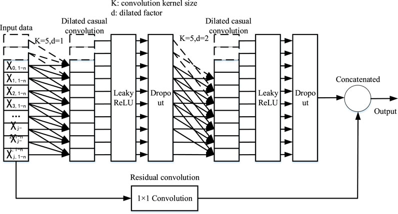
FIGURE 1. Flowchart of TCN residual convolution.
The historical data captured by a simple causal convolution is only linearly related to the depth of the network, which is a great challenge for sequential tasks that need to consider longer sequential dependencies. Vanilla CNN has a small receptive field to cope with such sequences. To address this, Yu and Koltun (2015) applied the classical dilated convolution neural network to exponentially expand the convolution receptive field). Specifically, for inputs x0, x1, x2…, xT and filters f:{0, 1, …,k − 1}, the dilated convolution in sequential series s could be represented as:
where d is the dilated factor and k is the size of filters, s-d(i) refers to the history. Dilated convolution is an effective strategy to increase the receptive field without increasing the kernel size or the number of parameters. When the dilation d = 1, the dilated convolution functions as a normal convolution. The larger the dilated factor is, the longer the input range. As a result, a better receptive field for the convolution network is achieved as shown in Figure 1. Consequently, the receptive field of the TCN can be freely enlarged by changing the dilation rate.
Despite the causal and dilated convolution used for the TCN, the model may sometimes encounter problems such as gradient disappearance. To address this issue, the TCN structure is made to be generic, motivated by the residual structure presented in ResNet (An et al., 2020). In this paper, the residual convolution takes X series of input, transforms them, and the results are concatenated with the input. Consequently, the output of the residual convolution is:
As shown in Figure 1, two layers of dilated causal convolution and activation function are included in a residual convolution. Moreover, dropout operation is used for regularization at each dilated convolutional layer. After that, 1 × 1 convolution is implemented for input X to ensure the same scale of tensors between inputs and outputs of residual convolution.
Experiment and System Architecture
Research Object
NPPs are composed of different components. Since the method proposed in this paper has not been verified through an engineering application, we select electric gate valves to evaluate the RUL predictive model. In NPPs, the valve is one of the most important components, used for flow control and to adjust the working fluid pressure. Research shows that the proportion of nuclear power plant shutdown due to valve failure is 19%, which is mainly caused by assembly defects, human factors, and operating environment. Apart from scheduled maintenance, the valve is generally not allowed to stop for inspection and its condition could only be detected from the outside i.e. through a nondestructive test. Moreover, for nuclear safety-related valves, due to the limitation of installation space and cost, there are limited redundant provisions. Considering the importance of electric gate valve to the safe operation of light and heavy water reactors, the run to failure data of the gate valve is taken as the training dataset to verify the effectiveness of the proposed RUL predictive model.
As shown in Figure 2, the electric gate valve used for this experiment is the Z941h-25P straight screw gate valve, driven by squirrel cage coil motor. Also, the diameter of gate valve is 50 mm while the truncation mode is rigid single gate with nominal pressure of 2.5 MPa. The experimental gate valves’ running conditions are configured to closely mimic what is obtainable in the real NPP operation.
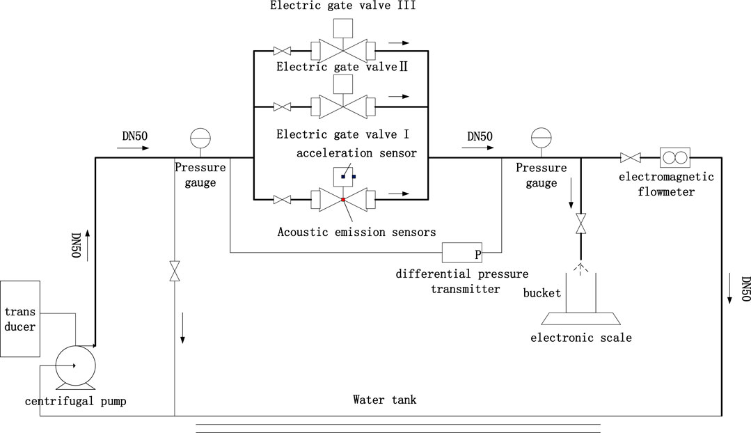
FIGURE 2. Illustration of the electric gate valves experimental platform.
In this paper, the external crack of the electric valve is selected as a typical fault mode. The main reasons for the crack are as follows: first, the uneven lattice of the valve plate or valve body leads to a material defect. Secondly, the uneven impact of the fluid or installation defects lead to uneven force on the valve plate or valve body. Thirdly, the fluid corrosion effect and the radioactive material irradiation lead to a corrosive hole that causes leakage. To preserve the valves for further experiments, and to ensure reproducibility and save cost, destructive cracks are not made on the valves during the experiment. Instead, certain reasonable assumptions and approximations are made to design the aging parts of the electric valve as shown in Figure 3. Three holes with 3, 5, and 10 mm are inserted and screwed on the valve body plate. During the experiment, the aging degrees are simulated by slowly adjusting the rotating screw.
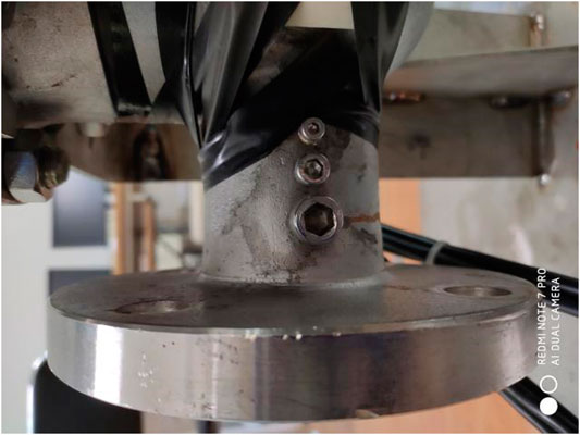
FIGURE 3. The electric valve studied in the experiment to simulate degradation.
For an accurate RUL prediction for electric valves, the selection of measurements to reflect the status of the electric valve is important. In this paper, the static pressure and pressure difference at the valve inlet and outlet is measured by static pressure and differential pressure gauge. The electromagnetic flowmeter is also used to measure the flow rate for analysis. To completely represents the aging state of the electric valves, other signal detection methods are used to measure the characteristic parameters. The acoustic emission methods use sensors to measure the transient stress waves on the surface of the valve body when cracks occur. When the valve runs normally, no acoustic emission occurs. After the valve show cracks or even leakage, fluid flow through the leakage produces jet turbulence, which in turn produces a continuous mechanical stress wave. The sensor mounting surface is polished with sandpaper in advance to remove any impurities. Details of the mounted valves, components, the experiment procedure, and circuit configuration can be found in Wang et al. (2015).
Model Architecture and Implementation Flowchart
The architecture of the RUL predictive model based on improved TCN described in this paper is shown in Figure 4. The whole process is divided into the training and actual RUL prediction phase:
Step 1. Feature engineering is carried out on the acquired data from the experimental platform. Irrelevant features are removed to ensure an effective and compact model. The selected features are normalized and standardized.
Step 2. To enable the algorithms to fully take into account the sequential characteristics, the original 2D (N * D) data collected is preprocessed and reshaped to 3D stacked data block in the form (n − num_steps +1) * num_steps * D, where N is the batch length, D is the features, and num_steps refers to sequence length of the time series. In this paper, the sliding window with length num_steps is adopted to the original 2D degradation data x. Since there is an overlap between slides of each window, the total input length is (n − num_steps + 1). In this way, the input data is not just a single data point but a sequence of time-series data, which better reflect the sequential characteristics of the degradation process.
Step 3. Unsupervised feature extraction by one-dimensional convolutional auto-encoder (CAE) is implemented. The theoretical analysis of CAE and its advantages can be found in reference (Wang et al., 2020c). The model is developed using the Tensorflow framework, where the encoding and decoding processes are implemented to form the deep feature representation.
Step 4. Results of the one-dimensional CAE are concatenated with the original data gathered from Step 2. By doing so, significant features in the aging data could be enriched to further develop an accurate RUL predictive model.
Step 5. The feature extraction results are transferred to the TCN network. On the Tensorflow framework, the TCN tuple model is first developed, which consists of 1D causal convolution with many layers. For each causal convolutional layer, the dilated function is used after each TCN to increase the model receptive field.
Step 6. The residual convolution described in Research Object is improved by concatenating the results of the convolution filter. Moreover, the leaky ReLU activation function and sparse dropout operation are also used instead of ReLU or Sigmoid activation function based on the previous impressive performance of the Leaky ReLU activation function on non-linear sequential datasets (Wang et al., 2020b).
Step 7. When the TCN tuple unit is developed, the stack function is adopted to construct the entire TCN network.
Step 8. During CAE and TCN training, the processed data is randomly shuffled to avoid overfitting and then input into CAE and TCN models.
Step 9. The loss function in this paper is the root mean squared error (RMSE). Adam optimizer is used as the training algorithm. During backpropagation processes, the learning rate at the first 5 iterations is set to 0.001 without attenuation. Then the attenuation rate of each subsequent iteration is set to 0.99. With increasing training epochs, the training errors decreases until it stabilized.
Step 10. When the off-line training process is completed, the randomly selected test data is normalized as shown in step 1 and step 2. Then, the optimized TCN models are used to predict the RUL of the electric gate valves. The model evaluation metrics are the explained variance score, mean absolute error, mean squared error, and R2 score.
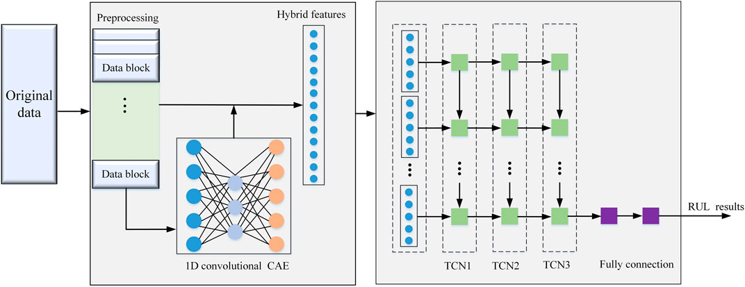
FIGURE 4. The complete architecture of the RUL predictive model.
Simulation Analysis
Data Acquisition
The degradation of the electric-valves is measured in the experiment. First, the water tank is filled as shown in Figure 2, and an electric valve loop is fully opened. The inverter for the pump is set to 15 kHz and its corresponding pump speed is about 870 r/min. The pipeline is filled with water after some time. Then, the driving pressure of the pipeline is 0.26 MPa, the valve is in normal operation, the pressure difference across the valve is 6 KPa and the total flow in the pipeline is 3 m3/h. Also, relevant parameters of acoustic emission cards are set as: sampling frequency-5,000 kHz, digital filter band-15∼70 kHz, the interval of parameters-500 μs, hangover time-1,000 μs, peak interval-300 μs, locking time-1,000 μs, single-channel waveform threshold-40 dB, and single-channel parameter threshold 40 dB.
In the experiment, the crack simulating screw is slowly adjusted under a certain pump frequency and the electric valve position (opening degree) to gradually increase the leakage. Different pump frequencies and opening degrees represent different operating conditions of the electric-valves. In this paper, a total of five different circulating pump frequencies (PF) and eight valve openings (VP) are set during the experiment with a total of 40 operating conditions. Under each operating condition, 30 groups of experiments are carried out with various levels of screw tightness. In each group of the experiment, the measured variables are the frequency of the circulating pump, opening degree of the electric-valve, pressure difference between the front and rear of the electric-valve, and the fluid flow rate through the valve. For acoustic emission signals acquisition, computer software is used to automatically calculate the amplitude, ringing count, rising time, energy, root mean square (RMS), average signal level (ASL), and other parameters.
Moreover, the length of time for each group varies from 2 to 3 h to provide adequate aging data. Figure 5 shows different variations of some selected conditions under which the acoustic emission sensors measurements were obtained. From the figure, the amplitude of acoustic emission parameters and ringing count all show approximately the same trend as the leakage volume increases under a certain pump frequency and valve opening position. When the leakage is less than a certain value, the relevant characteristic parameter has no significant deviation. However, when the leakage exceeds a threshold, the parameter presents an obvious change in trend. When the leakage further increases to a certain critical value, the parameter remains constant again. This is because when the leakage is tiny, the leakage has little effect on the flow in the pipeline. But, when the leakage becomes too large, the pipeline flow is no longer under turbulent states.
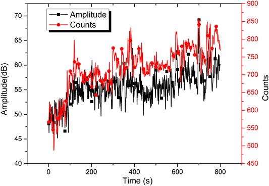
FIGURE 5. The trends of parameters with PF = 30 Hz, VP = 35%.
Comparison of Different Model Structures and Hyper-Parameters
For pattern recognition with deep learning, many trainable parameters directly influence the model performance. However, there are no generic hyperparameter selection criteria. Hence, it is necessary to analyze and compare different hyperparameters to obtain an optimal model for the RUL prediction.
Optimizable hyperparameters in TCN include the learning rate, learning rate delay factor, maximum iterations, batch number, selection of training algorithm, and dropout coefficient, among others. From the authors’ experience, the fine-tuning of these hyperparameters has little impact on the overall results. Therefore, the hyperparameters selected in this work is motivated by the performance recorded in recent literature. The default structure and hyperparameters of the proposed ITCN are shown in Table 1.
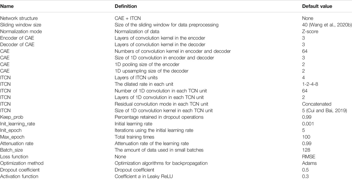
TABLE 1. The architecture definition of ITCN.
In addition to the above hyperparameters, we analyzed the effect of the CAE preprocessing layer and different dilation rates on the predictive performance of TCN. Finally, explained variance score (EVS), mean absolute error (MAE), RMSE, and R2 score metrics are obtained to evaluate the performance of the RUL predictive model.
With or Without Convolutional Auto-Encoder
First, an experiment is performed by adding the CAE layer without changing the structure of the proposed TCN, and the effect of the CAE layer is analyzed. Figure 6 shows the training and test curve for the specified epochs. It is seen that the network neither underfit nor overfit.
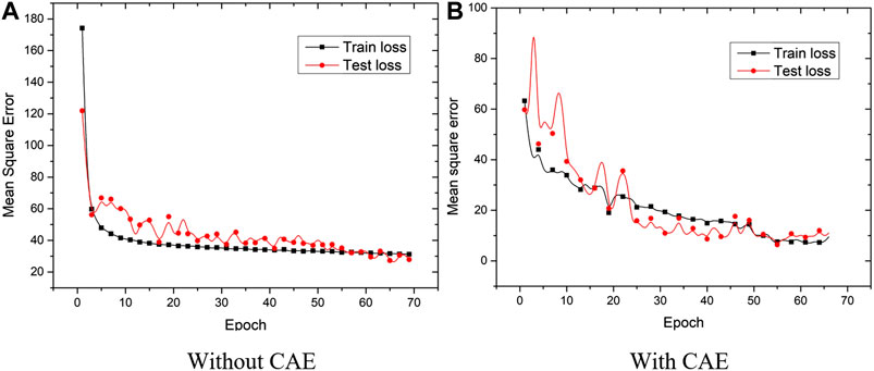
FIGURE 6. Training and testing curves with or without CAE.
Metrics are calculated for further analysis, as shown in Table 2. From the table, the metric for the model with CAE is better than that without CAE, which means CAE has a positive effect on feature extraction. Furthermore, after combining the feature extraction results of CAE with the original data, the explained variance score, RMSE, and R2 score are better than those without the parallel structure. This is mainly because after adopting the parallel structure of CAE and the original data, the dimension of the feature map expanded from the original 9 dimensions to 18 dimensions, which is equivalent to enhancing the feature performance. Therefore, the CAE layer has a significant effect on the improved TCN network for RUL prediction.
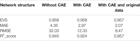
TABLE 2. Metrics with or without CAE.
Receptive Field With Different Layers and Dilated Factors
After evaluating the effect of the CAE layer, we compared a different number of causal convolution layers and the dilated factors for TCN optimization. As shown in Figure 1, two layers of dilated causal convolution and activation function are included in each causal convolution layer. Table 3 shows the comparison result. It is seen that the best metric for the predictive model is obtained when there is four causal convolutional layer and dilated factor is set to 1, 2, 4, 8. Therefore, it is concluded that this structure optimizes the RUL predictive model.
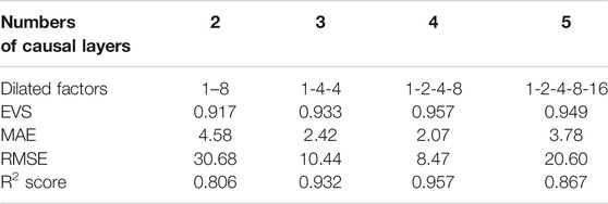
TABLE 3. Average test loss with different layers and neurons of CAE.
Comparison of the Proposed Method With Conventional Algorithms
To verify the performance of the proposed improved TCN model, a fully connected network (FCN), Convolutional Neural Network (CNN), LSTM model, and its variation were implemented and compared for the same dataset. For FCN, it adopts the full connection of neurons between different layers, which is different from the TCN network during the training process. Therefore, by comparing with FCN, the advantage of DNNs is demonstrated. Also, to show that the improved TCN method is better than other DNNs, this paper compared the results of CNN, LSTM, and TCN. The relevant comparison results are shown in Table 4. From the results, it is seen that the accuracy and performance of TCN are better than other networks on the task of predicting the RUL of electric gate valves. Moreover, two operating conditions are selected at random, and the predicted RUL curves obtained from different models are shown in Figure 7. The RUL prediction trend for the improved TCN is the closest to the real RUL, which shows that the best prediction is obtained from the improved TCN model. This result is also consistent with the metric shown in Table 4.
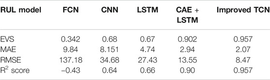
TABLE 4. Average test losses of different RUL prediction models.
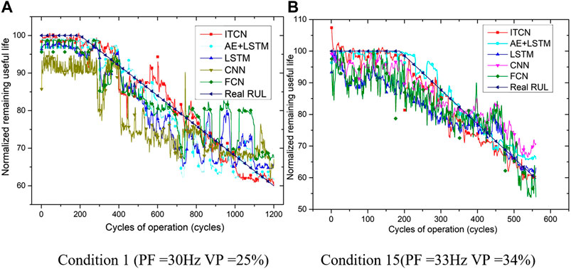
FIGURE 7. RUL results with different algorithms.
To further verify the predictive performance and demonstrate the generalization capability of the proposed improved TCN model, we also applied it to predict RULs for the turbofan engines in the NASA C-MAPSS benchmark datasets. The C-MAPSS dataset contains the degradation history of aero-propulsion engines operating under different fault modes. The dataset has four subsets composed of multi-variate temporal data obtained from 21 sensors. Detailed information on the composition of the dataset can be found in reference (Ramasso, 2014). Due to space constraints, we evaluated the proposed method only on the FD001 subset of the C-MAPSS dataset.
Similarly, the different methods mentioned in this section are compared. The relevant comparison results are shown in Table 5. It is seen that the improved TCN network still has the highest accuracy for FD001 data and all TCN evaluation metrics are better than other networks.
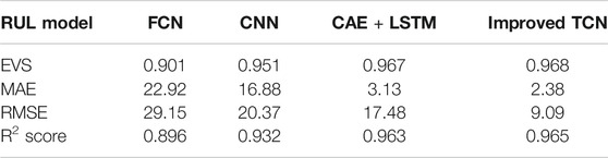
TABLE 5. Average test losses of different RUL prediction models.
Remaining Useful Life Prediction Results
This section presents the RUL prediction results under different aging conditions. As shown in Figure 8, the average RMSE of the improved TCN and the original TCN under different operating conditions are presented. It is seen that there is an impressive increase in accuracy of improved TCN compared with that of the original (vanilla) TCN under different operating conditions.
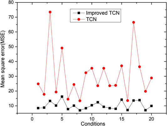
FIGURE 8. RMSE results of ITCN vs, vanilla TCN under different operating conditions.
Moreover, Figure 9 is the results of the RUL prediction curve after randomly selecting different operating conditions. It is seen that the RMSE in Figure 8 is consistent with the RUL prediction curve of the improved TCN, which is significantly better than the original TCN. Moreover, it can be seen that before and at the beginning of the equipment degradation, the errors between the predicted curves and the real curve is large, which is mainly caused by the sensor measurement error and noise during normal operation. With the gradual development of degradation, the improved TCN could better track the real RUL. As the equipment approaches the end of life, there is a minor deviation between predicted and real RUL but within the acceptable range.
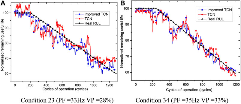
FIGURE 9. Results of RUL prediction under different operating conditions.
Conclusion
This work proposes an improved TCN (ITCN) model for nuclear power plant electric gate valve remaining useful life estimation. Multi-variate training datasets that represent the degradation history of the valve are acquired from an experimental platform. The dataset is subsequently preprocessed and normalized. High-performing convolution auto-encoder layers are also integrated into the ITCN model to improve model performance. Moreover, we experimented with different model hyperparameters and convolution dilation factors to determine the best parameters for the model. The research result and evaluation metric show the impressive performance of the ITCN model. To further verify the generalization capability of the proposed method, the model is evaluated on NASA’s C-MAPSS dataset, to predict RUL for aero-propulsion engines. Evaluation results show similar impressive performance on the benchmark dataset. The results also show that the work can be further extended to other mechanical components and devices. Other advantages of the proposed method are its ability to solve the problem of large computing resources and memory requirements that is common to LSTM and other RNNs. The originality of this study is summarized below:
(1) We present and analyze major issues that constraint the implementation of PHM for nuclear power systems
(2) We propose an improved TCN predictive model, based on CAE and improved residual convolution. The parallel structure of the TCN is augmented to enhance feature processing for accurate RUL prediction.
(3) The proposed method is extensively evaluated using aging characteristics of electric gate valves and other benchmark datasets. The RUL prediction result and the comparative analysis of other state-of-the-art models show an impressive performance of the proposed method.
The results also show that the proposed method can be applied to critical components and devices in other industries. It could also enable predictive maintenance which reduces maintenance downtime and part replacement cost, and improves productivity. Nevertheless, we observed some limitations of the research. First, the data acquisition procedure presented in this work needs to be optimized. Aging and degradation modes in experiments also need to be extended to completely reflect the real degradation process. Further, the proposed method needs to be verified using real degradation information from operating NPPs. Moreover, the hyper-parameters and layer numbers of the proposed ITCN are selected manually which is time-consuming. The application of heuristic optimization algorithms and auto-tuners could further optimize the predictive model performance. These limitations will be addressed in our future work.
Data Availability Statement
The raw data supporting the conclusions of this article will be made available by the authors, without undue reservation.
Author Contributions
HW: writing and tested RUL prediction algorithms. MP: designed the whole architecture. RX: experiment and acquiring data. HX: comparison with other typical methods. HS: writing and English grammar problem revision.
Funding
This work was supported by the Foundation project of nuclear power technology innovation center of science, technology and industry under Grant HDLCXZX-2019-ZH-036.
Conflict of Interest
The authors declare that the research was conducted in the absence of any commercial or financial relationships that could be construed as a potential conflict of interest.
References
An, Q., Tao, Z., Xu, X., El Mansori, M., and Chen, M. (2020). A data-driven model for milling tool remaining useful life prediction with convolutional and stacked LSTM network. Measurement. 154, 107461. doi:10.1016/j.measurement.2019.107461
Ayo-Imoru, R. M., and Cilliers, A. C. (2018). A survey of the state of condition-based maintenance (CBM) in the nuclear power industry. Ann. Nucl. Energy. 112, 177–188. doi:10.1016/j.anucene.2017.10.010
Bai, S., Kolter, J. Z., and Koltun, V. (2018). An empirical evaluation of generic convolutional and recurrent networks for sequence modeling. [Preprint]. arXiv :1803.01271v2 [cs.LG].
Chen, L. T., Xu, G. H., Zhang, S. C., Yan, W. Q., and Wu, Q. Q. (2020). Health indicator construction of machinery based on end-to-end trainable convolution recurrent neural networks. J. Manuf. Syst. 54, 1–12. doi:10.1016/j.jmsy.2019.11.008
Chiachío, J., Jalón, M. L., Chiachío, M., and Kolios, A. (2020). A Markov chains prognostics framework for complex degradation processes. Reliab. Eng. Syst. Saf. 195, 106621. doi:10.1016/j.ress.2019.106621
Coble, J., Ramuhalli, P., Bond, L. J., Hines, J. W., and UIpadhyaya, B. R. (2015). A review of prognostics and health management applications in nuclear power plants. Intl. J. Progn. Health Manag. 16, 2153–2648.
Cui, H., and Bai, J. (2019). A new hyperparameters optimization method for convolutional neural networks. Pattern Recogn. Lett. 125, 828–834. doi:10.1016/j.patrec.2019.02.009
Deng, S. J., Jia, S. Y., and Chen, J. (2019). Exploring spatial–temporal relations via deep convolutional neural networks for traffic flow prediction with incomplete data. Appl. Soft. Comput. 78, 712–721. doi:10.1016/j.asoc.2018.09.040
Downey, A., Liu, Y. H., Hu, C., Laflamme, S., and Hu, H. (2019). Physics-based prognostics of lithium-ion battery using non-linear least squares with dynamic bounds. Reliab. Eng. Syst. Saf. 182, 1–12. doi:10.1016/j.ress.2018.09.018
Gouriveau, R., Medjaher, K., and Zerhouni, N. (2016). From prognostics and health systems management to predictive maintenance 1: monitoring and prognostics. Editor A. EL Hami (London, UK: John Wiley & Sons), 15–26.
Hinchi, A. Z., and Tkiouat, M. (2018). Rolling element bearing remaining useful life estimation based on a convolutional long-short-term memory network. Procedia Comput. Sci. 127, 123–132. doi:10.1016/j.procs.2018.01.106
Huang, X. M. (2020). Intelligent remote monitoring and manufacturing system of production line based on industrial Internet of Things. Comput. Commun. 150, 421–428. doi:10.1016/j.comcom.2019.12.011
Jardine, A. K. S., Lin, D., and Banjevic, D. (2006). A review on machinery diagnostics and prognostics implementing condition-based maintenance. Mech. Syst. Signal Process. 20 (7), 1483–1510. doi:10.1016/j.ymssp.2005.09.012
Kundu, P., Darpe, A. K., and Kulkarni, M. S. (2019). Weibull accelerated failure time regression model for remaining useful life prediction of bearing working under multiple operating conditions. Mech. Syst. Signal Process. 134, 106302. doi:10.1016/j.ymssp.2019.106302
Lee, C. Y., and Kwon, D. (2019). A similarity based prognostics approach for real time health management of electronics using impedance analysis and SVM regression. Microelectron Reliab. 83, 77–83. doi:10.1016/j.microrel.2018.02.014
Lee, J., Ni, J., Djurdjanovic, D., Qiu, H., and Liao, H. T. (2006). Intelligent prognostics tools and e-maintenance. Comput. Ind. 57 (6), 476–489. doi:10.1016/j.compind.2006.02.014
Lin, Y. H., Li, X. D., and Hu, Y. (2018). Deep diagnostics and prognostics: an integrated hierarchical learning framework in PHM applications. Appl. Soft. Comput. 72, 555–564. doi:10.1016/j.asoc.2018.01.036
Mardar, E., Klei, R., and Bortman, J. (2019). Contribution of dynamic modeling to prognostics of rotating machinery. Mech. Syst. Signal Process. 123, 496–512. doi:10.1016/j.ymssp.2019.01.003
Mishra, M., Martinsson, J., Rantatalo, M., and Goebel, K. (2019). Bayesian hierarchical model-based prognostics for lithium-ion batteries. Reliab. Eng. Syst. Saf. 172, 25–35. doi:10.1016/j.ress.2017.11.020
Nguyen, K., and Medjaher, K. (2019). A new dynamic predictive maintenance framework using deep learning for failure prognostics. Reliab. Eng. Syst. Saf. 188, 251–262. doi:10.1016/j.ress.2019.03.018
Papadopoulos, C. T., Li, J. S., and O’Kelly, M. (2019). A classification and review of timed Markov models of manufacturing systems. Comput. Ind. Eng. 128, 219–244. doi:10.1016/j.cie.2018.12.019
Pawar, P., and Ganguli, R. (2007). Fuzzy-logic-based health monitoring and residual-life prediction for composite helicopter rotor. J. Aircr. 44 (3), 981–995. doi:10.2514/1.26495
Peng, K. X., Jiao, R. H., Dong, J., and Pi, Y. T. (2019). A deep belief network based health indicator construction and remaining useful life prediction using improved particle filter [J]. Neurocomputing. 361, 19–28. doi:10.1016/j.neucom.2019.07.075
Ramasso, E. (2014). Investigating computational geometry for failure prognostics. Int. J. Progn. Health Manag. 5 (1), 1–18.
Sato, M., Moura, L. S., Galvis, A. F., Albuquerque, E. L., and Sollero, P. (2019). Analysis of two-dimensional fatigue crack propagation in thin aluminum plates using the Paris law modified by a closure concept. Eng. Anal. Bound. Elem. 106, 513–527. doi:10.1016/j.enganabound.2019.06.008
Tang, D. Y., Cao, J. R., and Yu, J. S. (2019). Remaining useful life prediction for engineering systems under dynamic operational conditions: a semi-Markov decision process-based approach. Chinese J. Aeronaut. 32 (3), 627–638. doi:10.1016/j.cja.2018.08.015
Vichare, N. M., and Pecht, M. G. (2006). Prognostics and health management of electronics. IEEE T Comp. Pack. Man. 29 (1), 222–229. doi:10.1109/tcapt.2006.870387
Wang, B., Lei, Y. G., Yan, T., Li, N., and Guo, L. (2020a). Recurrent convolutional neural network: a new framework for remaining useful life prediction of machinery. Neurocomputing. 379, 117–129. doi:10.1016/j.neucom.2019.10.064
Wang, H., Peng, M. J., Miao, Z., Liu, Y. K., and Ayodeji, A. (Forthcoming 2020b). Remaining useful life prediction techniques of electric valves based on CAE and LSTM. ISA Trans. doi:10.1016/j.isatra.2020.08.031
Wang, S. X., Chen, H. W., Wu, L., and Wang, J. F. (2020c). A novel smart meter data compression method via stacked convolutional sparse auto-encoder. Int. J. Elec. Power. 118, 105761. doi:10.1016/j.ijepes.2019.105761
Wang, H., Ma, X. B., and Zhao, Y. (2019). An improved Wiener process model with adaptive drift and diffusion for online remaining useful life prediction. Mech. Syst. Signal Process. 127, 380–387. doi:10.1016/j.ymssp.2019.03.019
Wang, Y. F., Xue, C., Jia, X. H., and Peng, X. Y. (2015). Fault diagnosis of reciprocating compressor valve with the method integrating acoustic emission signal and simulated valve motion. Mech. Syst. Signal Process. 56–57, 197–212. doi:10.1016/j.ymssp.2014.11.002
Xia, T., Song, Y., Zheng, Y., Pan, E., and Xi, L. (2020). An ensemble framework based on convolutional bi-directional LSTM with multiple time windows for remaining useful life estimation. Comput. Ind. 115, 103182. doi:10.1016/j.compind.2019.103182
Yu, F., and Koltun, V. (2015). Multi-scale context aggregation by dilated convolutions. [Preprint]. arXiv:1511.07122v3 [cs.CV].
Keywords: remaining useful life prediction, electric gate valve, temporal convolutional network, residual convolution, nuclear power plant
Citation: Wang H, Peng M, Xu R, Ayodeji A and Xia H (2020) Remaining Useful Life Prediction Based on Improved Temporal Convolutional Network for Nuclear Power Plant Valves. Front. Energy Res. 8:584463. doi: 10.3389/fenrg.2020.584463
Received: 17 July 2020; Accepted: 08 October 2020;
Published: 06 November 2020.
Edited by:
Jun Wang, University of Wisconsin-Madison, United StatesReviewed by:
Khalil Ur Rahman, Pakistan Nuclear Regulatory Authority, PakistanCheng Liu, University of Wisconsin-Madison, United States
Copyright © 2020 Wang, Peng, Xu, Xia and Saeed. This is an open-access article distributed under the terms of the Creative Commons Attribution License (CC BY). The use, distribution or reproduction in other forums is permitted, provided the original author(s) and the copyright owner(s) are credited and that the original publication in this journal is cited, in accordance with accepted academic practice. No use, distribution or reproduction is permitted which does not comply with these terms.
*Correspondence: Hang Wang, d2FuZ2hhbmcxOTkwMzEyQDEyNi5jb20=