CFD-Based Wind Assessment for Suburban Buildings. The Case Study of Aarhus University, Herning Campus

The development in the field of wind turbines is continuously growing. However, most of the times, the energy of wind is exploited by using huge wind-power plants, while wind energy installations in urban and suburban areas, as space and available land, are a lot more limited, is something relatively new, with great potential though. The major challenge regarding small urban wind turbines can be summarized as a lack of understanding of the wind resource in the built environment, with a combination of missing measurements in this field that needed to be addressed. Aarhus University Campus Herning, located in the suburban area of Herning, is looking for a suitable place to install one small wind turbine (SWT). This study attempts to provide a comprehensive framework for SWTs and the characteristics of urban wind flow. The analysis helped in identifying the two most appropriate sites for SWTs installation sites in the AU Herning building.

Introduction

Background of the Research

The global energy consumption is estimated to increase between 2010 and 2040 by 56% (U.S. Department of Energy, 2016). Despite the decreasing coal, petroleum and natural gas resources, and all the issues their appliance evoke (such as global warming and climate change), in 2015, the share of fossil fuels was 78.4% of the final global energy consumption, while renewables and nuclear power accounted for only 19.3% and 2.3% (REN21, 2017).

On the 14^th of June, 2018 the European Commission, the European Parliament, and the Council agreed to set a new binding target of 32% final energy consumption from renewable sources by 2030 (European Commission, 2018). Conventional fuels are replaced with renewable energy in four distinct areas, namely, heating and cooling, power generation, transport fuels, as well as rural/off-grid energy services (Al-Bahadly, 2009; REN21, 2017; Hansen and Xydis, 2018).

The installed capacity of renewables was over 28% of the world’s total power-generating capacity by the end of 2016, which was more than 2000 GWs. 23% of the total renewable power capacity coming from wind power, was only preceded by hydropower (IRENA, OECD/IEA, and REN21, 2018). Generating 1 kWh power with wind energy saves approximately 800 g of carbon dioxide emission since that amount is rejected in the atmosphere during the combustion of fossil fuels (Bernard, 2001).

In urban and suburban areas, space and available land are a lot more limited, which sets a significant restriction against the establishment of larger plants. Wind energy installations close to buildings have received significantly less attention (Campbell and Stankovic, 2001; Beller, 2009; Sharpe and Proven, 2010). The idea of on-site micro wind energy generation is impressive considering the advantage that the energy is then being produced close to the location where it is needed (Xydis, 2015; Xydis and Mihet-Popa, 2016; Stathopoulos et al., 2018).

Despite the vast potential in wind energy, the technology for its utilization is not fully mature yet, although it is well established. Therefore, several areas require further improvements in order to reduce the cost of wind energy (Islam et al., 2013; Xydis, 2013). Some of the major barriers of wind farms include the lack of available sites, the high costs of investments in these systems, the impact of the grid on power quality, the degree of public acceptance, as well as the losses in power transmission when distributed to consumers (Musial and Ram, 2010). In order to reduce some of these barriers, one possible alternative can be the application of small wind turbine technology (Smith et al., 2012; Anup et al., 2018). Urban wind turbines can provide several benefits to the society, such as the generation of power right where it is needed, lack of transmission and distribution losses, the promotion of decentralized power and sustainable development, reduced greenhouse gas emissions, as well as the elimination of the dependency on grid electricity (Kumar et al., 2018).

Problem Statement

Within the built environment, small wind turbines (SWTs) can represent an excellent potential for integration. Research studies suggest that the reason for this growing uncertainty is closely related to poorly developed and unfounded decisions about the locating and positioning of urban wind turbines, which is supported by the lack of consideration regarding the accelerating effect that derives from the different heights of buildings as well as the surrounding urban configurations (Abohela, 2012; Suchada, 2012).

The potential of wind in urban areas and the technology that makes it possible to exploit this wind power through common models of turbines are studied in various case studies (Cace et al., 2007; Xydis, 2009; Ishugah et al., 2014). Studies also highlighted wind flow features in urban settings (Anup et al., 2018; U.S. Department of Energy 2015). According to Ledo et al. (2011), the main reasons for the limited establishment of SWTs in urban areas are the high intensity of turbulence, the low wind speeds, as well as the relatively high erodynamic noise, and displacement (Blackmore, 2010).

Another issue is that the direction of the wind changes frequently and there is a higher vertical inflow as well. The lack of understanding resulted in the improper use of SWTs and poor siting which can lead to potential turbine failure and liabilities (Smith et al., 2012). Therefore, the evaluation of wind power in urban and suburban areas is the biggest challenge regarding urban wind turbine projects, in which topic only a very few studies were conducted (Ishugah et al., 2014).

Aarhus University Campus Herning, located in Jutland peninsula, in the suburban area of Herning, is looking for a suitable place to install one small wind turbine.

Research Questions

This study attempts to approach and solve the real-life issue of Aarhus University, through the following research questions:

- How can CFD simulation be used in order to get a comprehensive picture of wind assessment within urban and suburban areas?

- How the optimal installation site can be determined for a small wind turbine within the area of Aarhus university Herning campus?

This study attempts to understand the effect of urban wind on the performance and loading of SWTs and facilitate decision-makers. It also deals with the appropriate installation location of SWTs in the built environment. The novelty of the study if focused on the simulation of a well-established phenomenon (fluid dynamics) in an intense and complex suburban environment. Literature and research findings are limited on the optimal siting of small wind turbines in university campuses (campi) and this is a piece of research covering this gap. The concept of small wind turbines has been around for long, however, challenges have not been thoroughly thought and opportunities have not been widely explored (Vilar et al., 2019). El Bahlouli and Bange (2018) experimentally and numerically had the opportunity to dig in the suburban campus buildings of the University of Tübingen. It was proven that the software based simulation results improved when the trees representation was considered as a canopy. Another study from Daniela et al. (2014), analyzed the wind resource in Transilvania University, in specific in the Colina Campus, where the profitability of installing small wind turbines in the campus area was revealed. Older studies, such as the one of Lu et al. (2011), and the one of Ozgur and Kose (2006), in practice tried with the available tools ten or more than ten years ago to prove the viability of small scale wind turbine projects in the Purdue University Calumet and in the Dumlupinar University. However, small wind turbines are more interesting for campi nowadays and we have decided to shed more light with this study.

The International Energy Agency has been documenting all the testing and research relating SWTs by requesting wind and turbine data of SWTs within the built environment from all of its member countries since 2013 (IEA Wind, 2017). Due to the broad aspect of several barriers associated to micro-site selection of SWTs in the built environment, this study needs to be narrowed down and focuses on one aspect of the site selection process, by using wind assessment data only.

The structure of this study is made up of five main sections, and the objective is to obtain a coherent picture of SWTs and the characteristics of urban wind flow, and to find the appropriate installation location of SWTs within the built environment following a deductive approach. After the introduction and the theoretical foundation of the study, the research methodology section follows, which provides a detailed explanation and description of the method and system of the research. The detailed description of the research itself comes after and in the last part the data collected in the previous section is analyzed, discussed, and evaluated, the research questions are answered, the conclusions of the research are drawn as well as the recommendations are made (Hevner, 2007).

Theoretical Background

Wind Characteristics and Urban Environment

In general, wind moves in a three-dimensional (3D) pattern from high to low atmospheric pressure areas. These differences in the atmospheric pressure and additionally, the rotation of the earth, develop currents within the atmosphere. These currents work as an enormous energy transfer medium (Ishugah et al., 2014). Urban boundary layer (UBL) is part of the planetary boundary layer, it is the layer where most of the Earth’s population lives now, and it has one of the least known and most complex microclimates. UBL has several impacts on urban airflow and the dispersion of air pollution, such as effects on thermal turbulence, local circulation systems, atmospheric stability, plume trajectories, convective structures, mixed layer depth, and on numerous other elements (Oke, 2015), such as air pollution (Arnfield, 2003; Barlow, 2014).

The UBL is characterized by the following features: Horizontal scales can be determined such as street (scale of 10–100 m), neighborhood (scale of 100–1000 m), and city (scale of 10–20 km). These scales can be explained as dimensions on which the urban structure becomes homogeneous, like an individual house or street, a group of buildings with similar shape and height within the same neighborhood or a town/city which is more rugged than the surrounding non-urban areas) (Oac.med.jhmi.edu, 2018).

In contrast with the open terrain of rural areas, the prevailing urban wind is defined by low annual mean wind speeds (AMWS) and rapidly changing wind direction with several obstacles, which causes more turbulent flow occurring in the atmospheric boundary layer (ABL). The low AMWS is the result of the uneven ground, while the increased turbulent flow originates from wind interacting with buildings and other obstacles (Mücke et al., 2011). As a result of the human-made surfaces’ high heat capacity, urban surfaces have significantly higher thermal inertia. This phenomenon leads to a non-negligible storage flux. In addition to the solar-driven energy balance, anthropogenic heat sources increase the sensible heat flux effectively. The urban roughness sublayer (RSL) can be defined as the atmospheric layer from the ground to approximately 2–5 times the mean building height (H). Within this layer, flow can be highly determined by space, it can be driven by turbulence which is affected by large-scale coherent structures. Close to the ground surface, Urban Canopy Layer (UCL) is formed by buildings. According to its determination, the layer ranges from the surface up to the average roof height.

At a neighborhood scale, roughness elements are continuously varying, and the flow continually adjusts to the ever-changing conditions. Due to the overlapping neighbourhood-scale, Interacting Boundary Layers (IBLs), these numerous changes of roughness result in a complex three-dimensional structure of the lower section of the UBL. Despite its complexity, it is essential to understand the function of the roughness sub-layer within the UBL, since being the interface between the atmosphere and the surface, is strongly affected by the activities of humankind. The Monin–Obukhov Similarity theory and other similar presumptions about flow and fluxes within the atmospheric surface layer (ASL) need to be abandoned, even though as a result of some progress more general characteristics are developing over the last decade (Pelliccioni et al., 2012). As buildings are 3D objects, as height increases, the speed of wind that flows around them increases as well, while the turbulence decreases. Simultaneously, whenever air collides buildings and other obstacles within the built environment, complex air vortex waves are developed as a result (Ricciardelli and Polimeno, 2006).

Airflow is measured in meters per second. Depending on the turbulence, two types of airflow can be distinguished: laminar (latin word “lamina” means straight), if there is no turbulence and turbulent flow when turbulence occurs (Testo.com, 2014). In order to translate the different flow types into mathematical models, a numerical description is crucial. The laminar and turbulent nature of the flow is determined by the value of the Reynolds number. It is a dimensionless number that predicts the fluid flows characteristics taking into account several properties such as viscosity, density, velocity, and so on. In the case of external flows, it can be observed that around the physical domain, the Reynolds number increases simultaneously, which concludes the presence of turbulent flow (Schechter, 1961).

When studying turbulence and its evolution in the UBL Turbulent Kinetic Energy (TKE) is one of the most critical variables to consider. If it is assumed that the flow can be separated into mean and turbulent parts, then the total kinetic energy of the flow is the sum of the kinetic energy of the mean as well as the turbulent flows. TKE is the mean kinetic energy/unit mass associated with currents in a turbulent flow. It can be expressed as follows:

$\mathit{TKE}=\overline{e}=\frac{1}{2}\left(\overline{u^2}+\overline{v^2}+\overline{w^2}\right)(1)$

where u, v, w are the velocity components.

SWTs

Only two wind turbine types are classified within the urban areas. These are the horizontal axis wind turbines (HAWTs) and the vertical axis wind turbines (VAWTs) (Chen et al., 2009). Although HAWTs are the most commonly applied types of wind turbines according to recent research, the VAWTs are more suitable for urban installation. As follows, HAWTs and VAWTs will be assessed based on the Wineur Project report (Cace et al., 2007) according to their advantages and disadvantages within the urban environment.

In urban applications, HAWTs do not outperform VAWTs, as VAWTs are almost as efficient as them, but HAWTs do not cope well with the increased turbulent flow. VAWTs, perform well in case of different wind directions and turbulence (Cace et al., 2007). They can multi-directionally rotate in turbulent flow, which makes them favourable within areas where the direction and speed of the wind frequently change (Elkhoury et al., 2015; Wineur, 2018).

With the tremendous development of information technology and hardware, three-dimensional modeling has also evolved over the years. In three-dimensional computer graphics, 3D modeling is the process that mathematically illustrates any three-dimensional objects. Modeling can be determined as the process of taking an object’s shape into a finished 3D mesh within a 3D environment as well (MediaFreaks, 2018). In their study, Gal et al. (2008) promoted the use of 3D modeling technologies within architecture, engineering, and construction industry. Xui-Gui (2008) applied the modeling software tool Sketchup to demonstrate how it increases the operating efficiency of the design, up to a certain extent.

Methodology

For studying this topic, potential research methods could be used, namely mathematical and statistical evaluation as well as computer simulations (Goddard and Melville, 2004; Saunders et al., 2007; May, 2011; Bryman, 2012). The former is mainly practical for handling large amounts of data since the examination of adequately selected parameters (such as mean values, distributions) can already be a sufficient foundation for some conclusions to be deduced. There is, however, a disadvantage of this method: it ignores the timeliness of each process. In order to overcome this problem, a set of computer simulation methods has been created that can be applied to examine input data with known timing as well. The approach has a deductive nature, as the aim is to select and gather already existing appropriate theories which are related to the investigated subject (Kothari, 2004; Wiles et al., 2011; Silverman, 2013).

Due to the fact that too many variables are defined in the problem statement, experimental research is necessary in order to fulfill the requirements for examining the results of slight modifications within well-defined and settled conditions, such as the CFD method (Saunders et al., 2007). On the other hand, by reason of the complexity, a retrospection was necessary to cover all the uncertain areas, which can be covered by the principles of action research (Hevner et al., 2004).

The research was conducted by performing the steps that are presented in the illustration shown in Figure 1. The research can mainly be divided into two connected main parts, the data collection and the numerical modeling respectively.

FIGURE 1

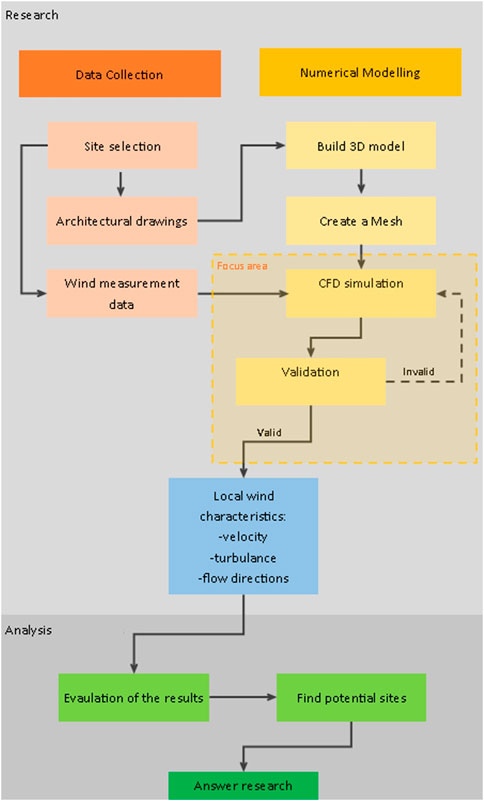
FIGURE 1. Methodology and research steps.

In his famous book, Principles of Operations Research, Wagner refers to simulation as the “...method of last resort...,” “...when all else fails....” However, since then, the popularity of computer simulation is growing, and it is now considered a serious and scientific methodology (Wagner 1975; Dooley, 2002; Kleijnen, 2017; Trochim, 2018).

When testing in real life is too expensive, dangerous or in situations when decision making is not feasible with the available information prediction is necessary (Kleijnen, 2017). In their book, Sargent et al. (2016) suggest various methods for verification and validation. However, this research focuses only on the use of metamodels. When running the simulation on metamodels, there should be signs that the simulation complies with the prior expert knowledge about the identical real system.

The Case Study of Aarhus University, Campus Herning

Specific Site and Wind Characteristics

The building of Aarhus University Campus Herning (later referred to as AU building) is used as the objective building, to assess the optimal installation sites for SWTs. The AU building is located in the Midtjylland region of Denmark (Figure 2A) within the suburb area of Herning, called Birk Centerpark (Figures 2B,C). The building is a standalone mixed-level structured construction, with 80 m in width (W), 25.2 m in height (H) and its longest extension (L) being 155 m. Therefore, it can be classified as a low-rize building, and according to its structural properties, it can be divided into three major parts, as follows:

- First part: a Six-story building containing the offices of the University (L 29.5 m × W 9.4 m × H 25.2 m) marked with A (Figure 2D)

- Second part: a two-story building which is rotated with 30 degrees—compared to the other two sections—for bigger lecture halls and community space (L 38.5 m × W 76 m × H 9.5 m) marked with B (Figure 2D)

- Third part: Two-story building for smaller lecture rooms (L 101.5 m × W 27.5 m × H 8.5 m) marked as C (Figure 2D).

FIGURE 2

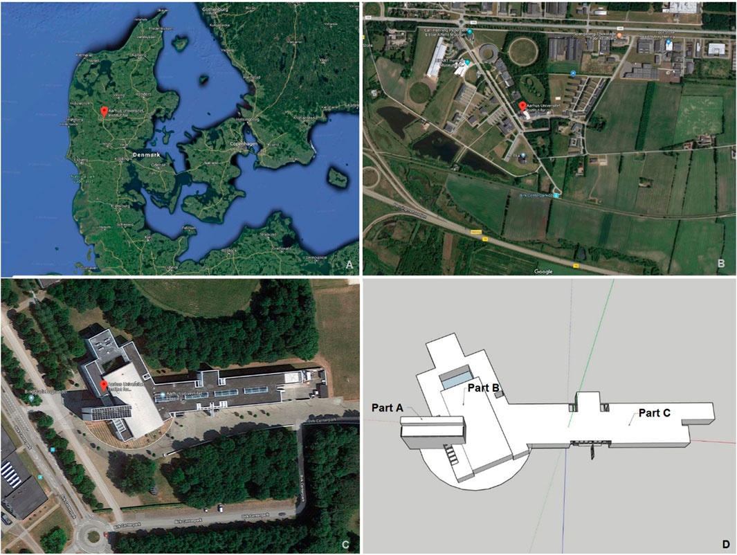
FIGURE 2. AU building/parts (A, B, C).

The most accurate data could be obtained by local measurements, however, due to limitations of this research, in the absence of these data, this study relied on online available sources. The first source is available from the website of the Global Wind Atlas (2019), where average data can be collected for the year in the area of the university. These data include velocity, wind roses at different heights.

The average velocity at 50 m and 100 m height can be seen on the figures below (Figures 3A,B). In addition to the above, surface roughness data are available as well, which may be necessary for more accurate wind profiling and selection (Figure 3C). The wind rose around the area of the University is defined in Figure 3D.

FIGURE 3

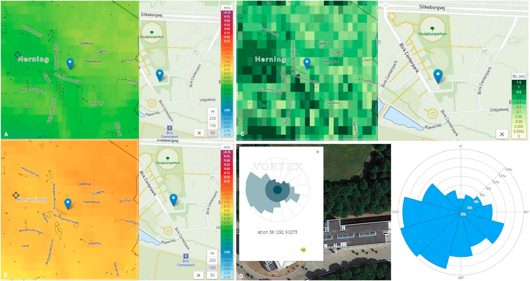
FIGURE 3. Average Velocity at 50 m (A), at 100 m (B), Surface Roughness (C), and wind roses (D).

The frequency of wind occurring in all of the directional sectors is indicated on the radial axis. To specify the corresponding predominant wind directions across the field the wind rose chart was applied. In order to use the above information with greater certainty, a private company’s data has been asked concerning the area of the site where the same velocity data was received. The wind rose is slightly different (Figure 3D—VORTEX wind rose), however, the deviation is minimal, since the 270-degree winds and the 240-degree winds fall in the same direction within the simulation. Based on this, it can be stated that the western wind direction is decisive in the area, therefore the focus will be put on this direction during the running of the simulation. To conclude, the facts for the simulation given based on the previous sections are the following:

- The site: Aarhus University’s standalone mixed-level structured building

- The main wind direction, which is 270 degree

- The velocity at 100 and 50 m height. The given values are 7 m/s and 5.75 m/s respectively

- The roughness level around the area is 0.3, since the surface of the AU building’s environment is almost flat with few surrounding trees.

3D Model Creation

The other necessary element is the 3D model of the AU building for the preparation of the simulation. For the construction of the 3D model, the building details and data were required for which the official layout plans of the AU building were received from the university. These plans made it possible to create the 3D model of the building with 0.1 m accuracy. As a starting point, the 3D models were created from the layout plans by using SketchUp, 2018 software. SketchUp is one of the most user-friendly and easy-to-use 3D modeling software that is widely used in architecture, engineering, film industry and video game design (SketchUp, 2018). Running the simulation requires a closed, watertight geometry (Download.autodesk.com, 2019), which is not supported by all formats. The construction that was obtained from SketchUp was transferred to the Rhinoceros 5 (Rhino) software. Rhino is a 3D computer graphics and computer-aided design (CAD) application software that can create, edit, document and render surfaces, bodies, point clouds, and polygon nets regardless of complexity and size. Due to their accuracy and flexibility, these models can be used in any process from illustration through animation to production. Therefore, the model was converted in this program, and the final format used for the simulation was Rhino file format (LLC, 2018).

Simple building geometries were used for the AU building model without facade details. The reason for the simplification is the fact that in case of a mesh creation it is more efficient to keep the number of edges as low as possible. Otherwise, as a result of a greater amount of edges, it would be necessary to generate a higher resolution mesh, which means that more calculations should be taken during the simulation and these effects would increase the duration process as well as the expense of the process. The 3 d model of the school can be seen in the following illustrations (Figures 4A–C).

FIGURE 4

FIGURE 4. AU Building 3D Model (direction x-y-z).

Mesh Generation

A mesh is a discrete representation of a geometric domain. Mesh can be identified as a bounding box (using sub-domains e.g. tetrahedra or hexahedra in 3D), where during the simulation, the calculations are made (Frey and George, 2013). To identify its extensions, a simple calculation can provide some help, which can also be used regarding wind tunnel and mock-up sizing. The dimensions of the fluid domain can be seen in Figure 5.

FIGURE 5

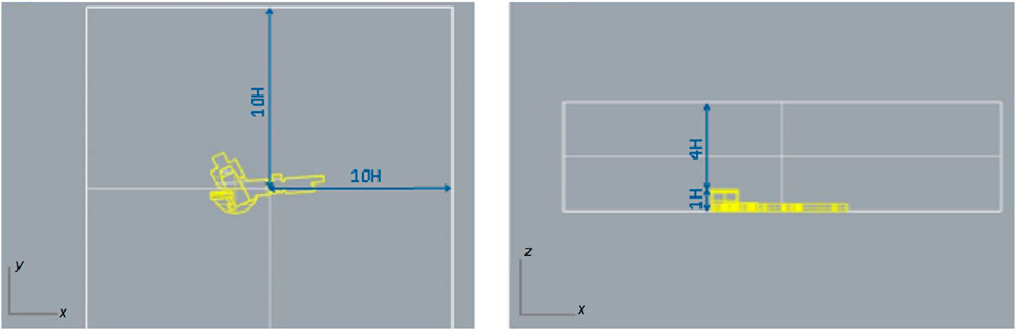
FIGURE 5. Mesh dimensions.

The number of infinite points, needs to be reduced to a certain amount of simply defined and controlled volumes in order to provide a feasible background for the mathematical calculations (Gokhale et al., 2008). Therefore, in this study, a hex-dominant parametric algorithm is used to decompose the fluid domain into 3D objects. The following steps were used:

- Region refinement: for the refinement of the region, a cylinder was defined around the building’s geometry, in order to identify that particular region as the most important, which also means that out of the given cylinder, a smaller number of 3 d objects are generated. In this case, as well, the scale is from zero to five, and a level of four can be seen in the following example (Figure 6A).

- Surface refinement: On the surfaces of the investigated geometry, the most diverse results are focused around the surface edges and corners. Thus, the refinement level for these polygons can be determined on a scale from zero to five. In this case the value is three to five, where five is the greatest value. It can be seen in Figure 6B. Finally, the last step is to determine the refinement for the outer bounding box, which is out of the cylinder, at a level of 2.

- It was necessary to run a grid independence test to analyze whether the result depends on the mesh grid or not. Therefore, the mesh size was varied from coarse to fine while the simulations were running with the same settings. The results are shown in Table 1; Figure 7. We could find that case 1 and 2 have too coarse grid, since the result variations are not significant after case 3. This mesh size can be considered as optimal in relation to the results and the number of calculations needed during the simulation.

FIGURE 6

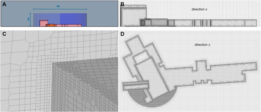
FIGURE 6. Region (A) and Surface (B) Refinement/Mesh Illustration direction x (C) and z (D).

TABLE 1

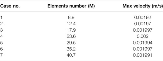
TABLE 1. Grid independence analysis.

FIGURE 7

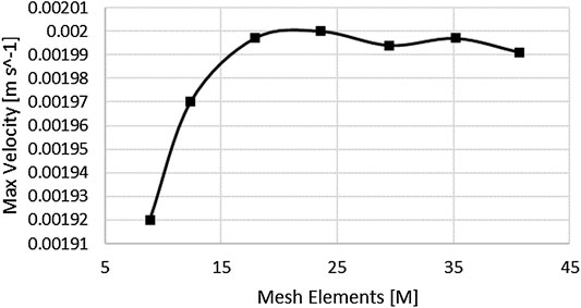
FIGURE 7. Max velocity compared to mesh elements.

With this method, a sufficient mesh can be achieved, which has a high level of 3D object density around the investigated surfaces, while in general low level in the outer areas. It takes approximately 45 h to generate such a mesh with a 4-core computer. It has 17,891,809 volumes in total. The detailed illustrations of the mesh can be found in Figures 6C,D.

CFD Simulation

In order to set up a sufficient simulation, there are several critical points that need to be met. Since there is a pre-defined method to follow, it makes it easier to check whether all previous conditions are fulfilled or not. All CFD simulations require a 3D model or geometry as a foundation, besides that it is indispensable to have a fluid domain, as a boundary for the simulation itself. To establish a valuable simulation, different levels of input data are required. The first option that can be chosen is the input material, namely the physical volume which is the subject of the flow simulation (air). Viscosity values, should be applied as follows:

Viscosity model: Newtonian

Kinematic viscosity (v): 0.000015295 m²⁄s

Density (p): 1.1965 kg⁄m³

The implementation of different turbulence models into CFD methods has a significant impact on the outcomes, therefore it is substantial to select an appropriate model, which will simulate the reality as accurately as possible. In this case, the grid size, the number of time steps, and the Reynolds number dependence provide a good direction toward a method called Reynolds averaged Navier-Stokes equations (RANS) (Girimaji, 2005). Within this method, a popular and commonly used model is called K-omega shear stress transport (SST), which uses a two-equation model in order to include the turbulent kinetic energy and its dissipation. It also covers the wall functions within the simulation, and the combination of k-epsilon and k-omega behaviors in the outer region and the inner boundary layer (Menter, 1994).

After defining the volume of the flow, the boundary conditions should be characterized as well. Figure 8 contains all the applied properties.

FIGURE 8

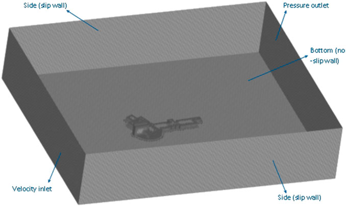
FIGURE 8. Outer Boundary Box.

FIGURE 9

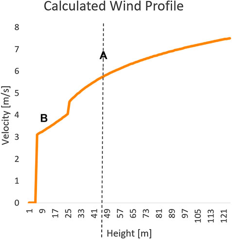
FIGURE 9. Wind profile.

The significant wind direction is at θ = 270°, in accordance with that, the velocity inlet is defined for the western side of the bounding box. One of the greatest challenges is to setup the velocity inlet, as well as to include the wind profile which should also reflect on the surrounding area.

One challenge is to specify the effects of the ground roughness on the lower level of the wind profile. However, as it is argued by Balczó and Tomor (2016), a roughness level below 0.5 has no significant consequences or effects on the development of wind profile (Balczó and Tomor, 2016). Nevertheless, it is essential to determine a level, so called zero-plane displacement (d), which can be determined as height in meters above the main surface level, where the velocity equals 0 due to surrounding obstacles in the flow (Burton et al., 2011). In order to represent the vegetation around the building, this value can be identified with the three-fourths of the average canopy height. Therefore, regarding the present setup, a logarithmic wind profile is used, and in order to reach proper accuracy, is made up of two sections. The first section is an exponential profile, where the previously defined value (d) is considered, while the second part is a logarithmical wind profile above the highest point of the building.

In order to solve the following equations, as a first step it is necessary to identify the friction velocity (u*), which can be calculated as follows:

$u_{\ast }=\frac{k\left(u\left(z2\right)-u\left(z1\right)\right)}{\ln \left(z2-d/z1-d\right)}(2)$

$u_{\ast }=\frac{0.41\left(7\text{m}/\text{s}\left(100\text{m}\right)-5.75\text{m}/\text{s}\left(50\text{m}\right)\right)}{\ln \left(100\text{m}-5\text{m}/50\text{m}-5\text{m}\right)}=0.686\text{m}/\text{s}(3)$

In these equations, (k) is the Von Kármán constant, which equals 0.41, while (z1) and (z2) are the measurement point heights. These are 100 m and 50 m respectively. The value for (d), can be specified as above, where the average canopy height is at 7.5 m, therefore the value of (d) can be determined as 5 m in this particular case. The logarithmic part of the wind profile can be calculated with the use of friction velocity as follows (a—on Figure 9):

$U\left(z\right)=\frac{u^{\ast }}{k}\ln \left(\frac{z-d}{z_0}\right),(4)$

$U\left(z\right)=\frac{0.68\text{m}/\text{s}}{0.41}\ln \left(\frac{z-5}{\mathrm{1,3}}\right)(5)$

In this equation, (z) is the reference height.

The exponential part of the wind profile can be calculated as follows (B – on Figure 8):

$U\left(z\right)=U_{\text{ref}}\exp \left(\alpha \left(\frac{z}{z_{\text{ref}}}-1\right)\right)(6)$

$U\left(z\right)=5.75\text{m}/\text{s}\exp \left(0.7\left(\frac{z}{50\text{m}}-1\right)\right)(7)$

Here, the attenuation coefficient (α) depends on building morphology, which can be determined as it is stated by Macdonald (2000), which is 0.7 in this particular case. As a result, sections of the excel data can be found in Table 2, as well as the wind profile (Figure 8).

TABLE 2

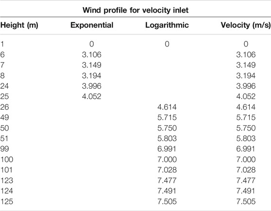
TABLE 2. Calculated wind profile.

For the remaining boundary layers, the wall functions are important to be classified. The top as well as the two slide walls, are “slip” walls, which means that it allows the initiation of a better simulation, even when compared to wind tunnel simulations, since the incompressible air will not circulate back from the side walls. The bottom part as well as the geometry itself are “no-slip” walls, therefore, the air is not able to penetrate through, and pressure can be measured on those surfaces as well. Consequently, in order to maintain the realistic airflow, the pressure outlet needs to be placed at the opposite side of the velocity inlet. The following step is to define the numeric within the simulation run, where the determination of the Courant-Friedrisch-Lewy number (C) has the utmost effect. In general, it is a condition for the stability which is used in any unstable numerical calculations, such as the CFD method. It has a connection with the definition of the data writing time set, since it is avoidable to write data files slower than the applied velocity. The reason can be seen in the following equation:

$C=\frac{u\Delta t}{\Delta x}=\frac{\text{physical}\text{domain}}{\text{numerical}\text{domain}}\le 1(8)$

In this equation, velocity (u) times the timestep between writing data, and (x) is the size of the cells, namely the 3D objects of the mesh. Therefore, the equation suggests, that the Courant number must be lower than 1, in order not to skip data writings between mesh objects, which leads to simulation termination. The shortening of the wiring steps has a huge effect on computational time, and as well a higher demand on the hardware. The other solution in this case is to increase the value of (x), by creating a lower quality mesh, which, in turn, also has a disadvantage as discussed in the mesh generation subsection. The smallest object on the created mesh is 9 cm, and the 0.7 Courant number classified as stable. The following equation shows that the numerical setup is feasible.

$C=\frac{5.75\text{m}/\text{s}\ast 0.001\text{s}}{0.0082\text{m}}=0.7(9)$

Another important setup option is related to the timeframe, which means how long should a simulated scene run. In this case, the termination time set to 3600 s. With the above described setups, running the simulation takes exactly 1,280 min when running on a 4-core computer. As a result, a dataset is available for post processing, which takes up more than a massive 31 GB of space.

Validation

This step has huge importance, to obtain reliable data through the simulation. A common practice to validate numerical calculations is to translate the applied process onto a well-known analyzed and simplified form (Sargent et al., 2016). Therefore, in order to validate the simulation (since there are no real-life wind measurements), a separate running flow is necessary to take on a standard cube with the same settings as it is used for the AU building.

From the result dataset, similarities have to be drawn both on the calculated results and flow streams around the cube. As a reference, the following two studies have been used for comparison. The first illustration (Figure 10A) shows how the airflow separates as it hits the obstacle. Two vortexes are also visible, which are very distinctive. The second graph shows how high and low velocity areas are built up around a cube (Figure 10B). Compare to these two figures, the simulation results on the test cube seems relevant (Figure 10C) (Gao and Chow, 2004; Lim et al., 2008).

FIGURE 10

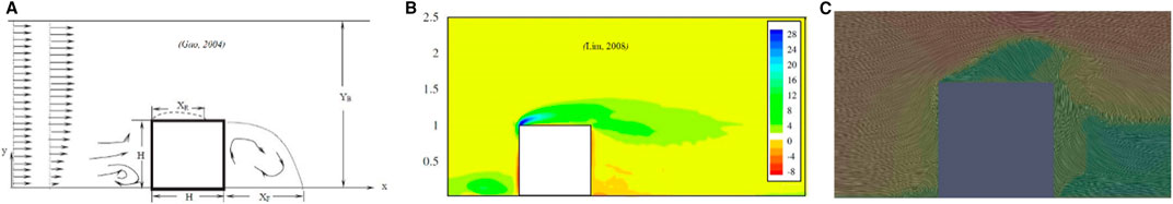
FIGURE 10. Flows around a test cube.

Analysis

Post Processing

As a result of the simulation, an enormous amount of data were available. Thus, it was necessary to follow the steps beneath, and answer the research question; a) extract the data: as soon as a simulation is completed without an error, we can access and extract the dataset, b) process the data: at this step, data conversion is needed, and as a result, the simulation data can be shown in different graphs and illustrations. The open source tool ParaView was used for post-processing. The visualization of the data was challenging, since for each desired parameter, a serial and parallel connection of subtractive filters were needed.

Evaluation of Results—Step 1

Exclude Unsuitable Areas

Under normal circumstances, whenever an airflow hits an obstacle that appears in its way, a separation can be observed. Right after the obstacle, reattachment can be expected, and within this area, high turbulence. However, on the other hand, as the air gets compressed during this separation, a change will occur in the velocity as well. To be able to identify the prior installation point, the regularities, as mentioned earlier, can be used. It is sufficient to exclude those areas already, where low velocity with high turbulence can be detected. Apparently, for appropriate decision making, a qualitative test is required.

For the SWTs, the cut-in speed is usually between 2–3 m/s. Therefore, those areas can be excluded from the list of possible locations, where velocity results stay beneath that certain level. To represent this data during post-processing, several filters are needed.

Since turbulent airflow has an adverse effect on the power output of SWTs, it is necessary to investigate those areas where the intensity is on a lower level. In order to reach that, an isovolume filter can be applied, whereas a fix value k = 0.4 m²s² is defined. Thus, the boundaries of turbulence kinetic energy (TKE) can be explored. The combination of the two results, high velocity, and low turbulence, can determine, and narrow down the possible installation sites.

Building Part A

In this section, the tallest part of the AU building, part A (Figure 11A), was investigated. As it can be seen on the velocity isovolume illustrations (Figure 11B), only the lower part of the top of the building has results of less than 3 m/s. Therefore, from this point of view, the upper top part of the building should be suitable for installation. The TKE (Figure 11C) is also low in those areas, so two possibilities should be investigated further.

FIGURE 11

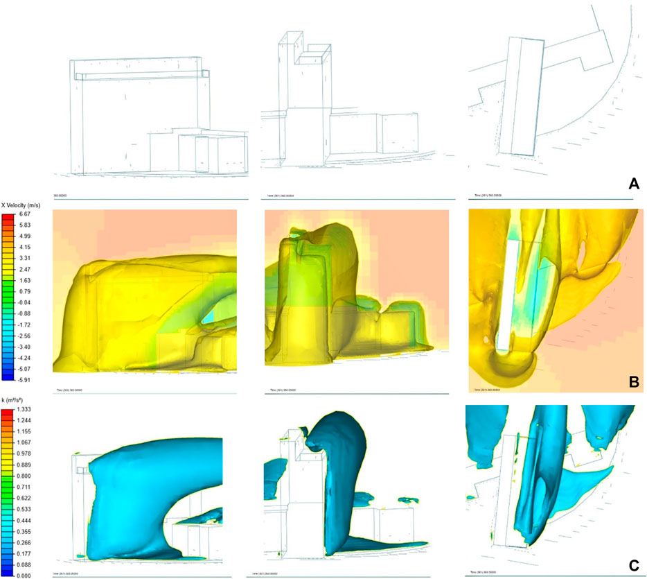
FIGURE 11. Building A (direction X, Y, Z) (A) – velocity (B) and TKE (C) isovolume.

Building Part B

The middle part of the AU building is broad in range, and it has a more significant extension in depth as well (Figure 11A). Velocity and TKE isovolume analyses are shown in Figures 12B,C. Since the A part cuts the middle, it has a substantial effect on the wind flow above the building. Thereafter, these four possible installation points are going to be considered later.

FIGURE 12

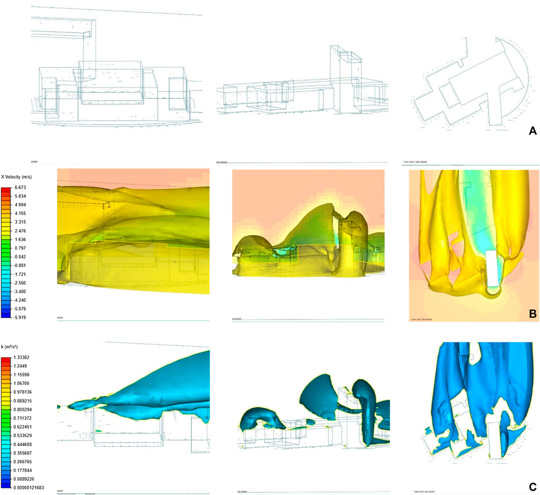
FIGURE 12. Building B (direction X, Y, Z) (A) – velocity (B) and TKE (C) isovolume.

Building Part C

Finally, the last section, part C, has a relatively wide dimension (Figure 13A). Unfortunately, as opposed to building B, this section of the AU building is almost entirely hidden from the favourable 270-degree wind flow, because of the covering of building part A. As it can be seen on both velocity (Figure 13B) and turbulence illustrations (Figure 13C) there is no location to select regarding feasible installation.

FIGURE 13

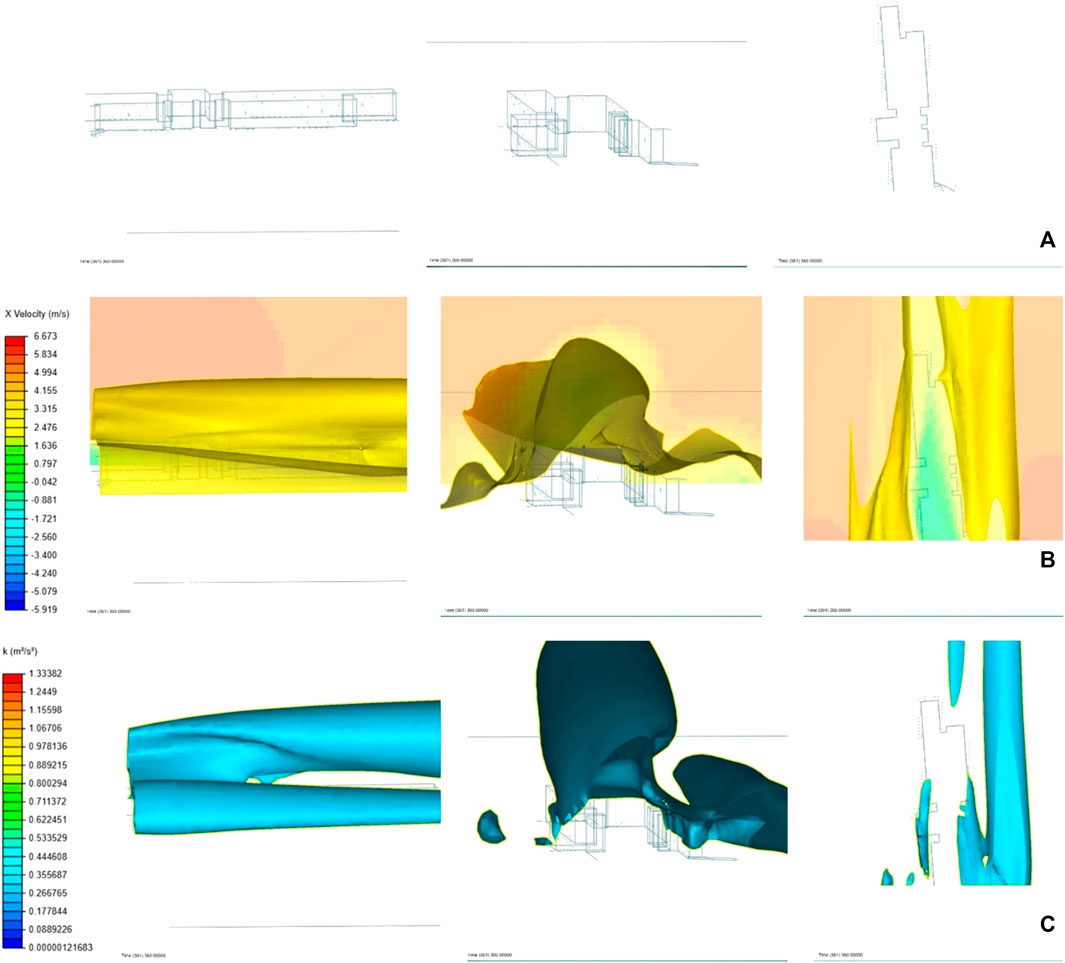
FIGURE 13. Building C (direction X, Y, Z) (A) – velocity (B) and TKE (C) isovolume.

The list of the narrowed suitable for SWTs points and its locations are presented in Table 3 and in Figure 14.

TABLE 3

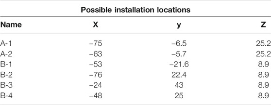
TABLE 3. Possible installation locations.

FIGURE 14

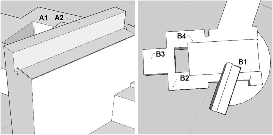
FIGURE 14. Building A and B (possible locations).

The following aspects should be considered during the second step of the evaluation:

- During the simulation, a 60 min period was conducted, so each result for each time step needs to be applied.

- The result should include the average of a larger area of the mesh in order to take the diameter of the turbine into account. Thus a 2.5 m times 2.5 m square is taken from the mesh for each point.

- Since the tower height of the turbine can vary, data should be presented from several different heights. In this case, five different heights were identified. By using the above-described method, the data extraction and visualization contains 40 elements for each possible installation point. The structure of these data can be seen in Figure 15A.

FIGURE 15

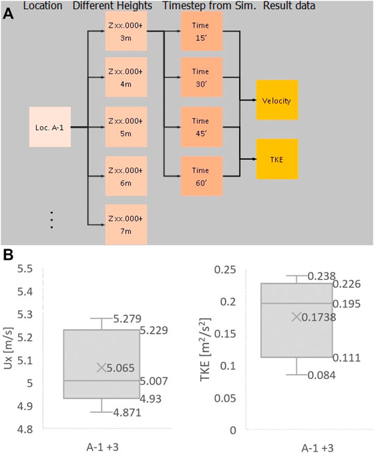
FIGURE 15. Data structure (A) and A1 average velocity and TKE (z + 3) (B).

Average Velocity and Turbulent Kinetic Energy

With the use of the already specified ParaView software, the average data values can be exported for each pre-defined mesh clips, so eventually, it is possible to visualize the average values on each location at each height levels (example in Figure 15B).

The data can be clustered based on the different parts of the AU building since the measured points have the same (z) coordinate values. In the Supplemenatary Appendix, the accumulated results combined for building part A (Supplementary Appendix Figures A1–A10), also, for building part B (Supplementary Appendix Figures A11–A20) and a graphical representation of the results (Supplementary Appendix Figure A21) can be found.

From the two selected points on building part A, at lower heights there is no significant difference between the two installation points, however, as the height increases, the velocity value grows slower on the second point (A-2). Moreover, the turbulence ratio is getting higher. Therefore, from those two points (A-1) provides better wind flow characteristics. Impressive results can be discovered on the other building, so in order to conclude all the details, each of them will be evaluated separately below.

- B-1 Velocity value starts at a reasonable level (compared to the calculated velocity at the same height) but, with higher turbulence. However, after reaching the height of (z) + 5, the turbulence flow starts to decrease, and velocity has a sharp increase in parallel.

- B-2 At the back of building section A, it starts on a higher velocity level, compared to B-1, however, during height increase, the turbulence flow will increase and therefore, the velocity value will drop slightly.

- B-3 at the height of (z) + 3 has good results regarding turbulent flows. Most probably it has no wind acceleration effect thanks to the fact that there are no surrounding buildings. Therefore, the velocity level remains on a lower scale, compared to the other points of building part B.

- B-4 had a great velocity value at (z) + 3, however as soon as it reached (z) + 5 height level, the turbulent flow out-powers the high velocity flows.

The following table contains the summarized results (Table 4), and in the last row, another calculation regarding the wind acceleration factor, which can be calculated with the following equation:

$Cv=\frac{U\left(z\right)}{U_0\left(z\right)}-1(10)$

where U(z) is the velocity result from simulation, and U₀(z) is the calculated wind (. CFD Simulation) velocity at the same height. Thus, the higher the number, the better the wind accelerating factor.

TABLE 4

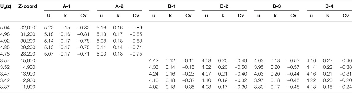
TABLE 4. Summarized results.

Based on the above-presented simulation results, there are two locations which show good properties for the possible turbine installation. One of them is at the top of the AU building, where, due to the great height, uninterrupted high-velocity flow can be reached. However, there is another possible location, which is situated at the front part of building part C. It is expected, that around the middle of building part A, there is a wind acceleration area, thanks to the building facing direction, and due to the western wind flows. In the case of height restrictions, point B-1 should be considered as a great installation point regarding the area’s wind characteristic nature.

Conclusion

The study was able to contribute to the understanding and solving of the leading research problem as well as to facilitate decision-making for given issue of AU Herning. It is essential to stress, that the particular area in this research is not a typical, dense urban area, as it is located in a suburban area of a city. The studied building itself is a standalone building and even the constructions located within its close environment are not that considerable. According to other studies, as well as the validation of this research for isolated buildings and small groups of buildings the simulation gives reasonably accurate results with a relatively low error level (Reiter, 2008).

It is also important to emphasize that this study only attempted to answer what is the most optimal installation site with regard to the wind conditions. For the selection of the installation point, a two-step method was used. In the first step by defining the high and low turbulence areas, it was possible to reduce the location of possible installation points, while, in the second step, the quantitative analysis of these points followed. Thus, given the so-obtained points taking into account all the results collected by the simulation, the ideal site location points are either location point A-1 or B-1.

Data Availability Statement

Publicly available datasets were analyzed in this study. This data can be found here: Global Wind Atlas (https://globalwindatlas.info/).

Author Contributions

DS performed the software simulations and GX conceived the initial idea. DS analyzed the data and wrote the draft paper. GX supervised and reviewed the paper.

Disclaimer

Frontiers Media SA remains neutral with regard to jurisdictional claims in published maps and institutional affiliations.

Conflict of Interest

The authors declare that the research was conducted in the absence of any commercial or financial relationships that could be construed as a potential conflict of interest.

Supplementary Material

The Supplementary Material for this article can be found online at: https://www.frontiersin.org/articles/10.3389/fenrg.2020.539095/full#supplementary-material.

References

Abohela, I. (2012). Effect of Roof Shape. Wind Direction, Building Height and Urban Configuration on the Energy Yield and Positioning of Roof Mounted Wind Turbines. PhD thesis. Sydney (Australia): Newcastle University.

Al-Bahadly, I. (2009). Building a wind turbine for rural home. Energy Sustain. Dev. 13 (3), 159–165. doi:10.1016/j.esd.2009.06.005

Google Scholar

Anup, K., Whale, J., and Urmee, T. (2018). Urban wind conditions and SWTs in the built environment: a review. Renew. Energy 131, 268–283. doi:10.1016/j.renene.2018.07.050

CrossRef Full Text | Google Scholar

Arnfield, A. (2003). Two decades of urban climate research: a review of turbulence, exchanges of energy and water, and the urban heat island. Int. J. Climatol. 23 (1), 1–26. doi:10.1002/joc.859

CrossRef Full Text | Google Scholar

Balczó, M., and Tomor, A. (2016). Wind tunnel and computational fluid dynamics study of wind conditions in an urban square. Theodore von Kármán Wind Tunnel Laboratory 120 (2), 199–229

CrossRef Full Text | Google Scholar

Barlow, J. (2014). Progress in observing and modelling the urban boundary layer. Urban Clim. 10, 216–240. doi:10.1016/j.uclim.2014.03.011

Google Scholar

Beller, C. (2009). Urban wind energy -state of the art 2009, RISOE-R-1668 (EN), risø DTU, national laboratory for sustainable energy. Roskilde, DK: Technical University of Denmark.

CrossRef Full Text | Google Scholar

Bernard, J. (2001). Le gaz naturel remonte le courant. Sci. Vie 214, 68–73.

Google Scholar

Blackmore, P. (2010). Building-mounted micro-wind turbines on high-rise and commercial buildings. Editor B. R. Watford UK IHS BRE Press.

Google Scholar

Bryman, A. (2012). Social research methods. 5th Edn. Oxford, UK: Oxford University Press.

Google Scholar

Burton, T., Sharpe, D., Jenkins, N., and Bossanyi, E. (2011). Wind energy handbook. Chichester, WS: John Wiley and Sons, Ltd.

Google Scholar

Cace, J., ter Horst, E., Syngellakis, K., Niel, M., Clement, P., Heppener, R., et al. (2007). Urban wind turbines- guidelines for small wind turbine in the built environment. WINEUR. Available at: www.urban−wind.org, 1–41.

Google Scholar

Campbell, N. S., and Stankovic, S. (2001). A report for Joule III Contract. Wind energy for the built environment – project WEB. .

Google Scholar

Chen, Z., Guerrero, J., and Blaabjerg, F. (2009). A review of the state of the art of power electronics for wind turbines. IEEE Trans. Power Electron. 24 (8), 1859–1875. doi:10.1109/tpel.2009.2017082

Google Scholar

Daniela, C., Radu, S., Codruta, J., and Oliver, C. (2014). Wind potential analysis in brasov built environment. Appl. Mech. Mater. 659, 337–342. doi:10.4028/www.scientific.net/amm.659.337

CrossRef Full Text | Google Scholar

Dooley, K. (2002). “Simulation research methods,” in Companion to organizations (London, United Kingdom: Blackwell).

CrossRef Full Text | Google Scholar

Download.autodesk.com. (2019). Tracking down watertight problems. [online] [Accessed 10 November, (2019).

Google Scholar

European Commission (2018). Renewable energy—energy—European commission. Available at: https://ec.europa.eu/energy/en/topics/renewable-energy. [Accessed 5 August, 2018].

Google Scholar

El Bahlouli, A., and Bange, J. (2018). Experimental and numerical wind-resource assessment of a university campus site, Green Energy and Technology. PartF 10, 1–15. doi:10.1007/978-3-319-74944-0_1

Google Scholar

Elkhoury, M., Kiwata, T., and Aoun, E. (2015). Experimental and numerical investigation of a three-dimensional vertical-axis wind turbine with variable-pitch. J. Wind Eng. Ind. Aerod. 139, 111–123. doi:10.1016/j.jweia.2015.01.004

CrossRef Full Text | Google Scholar

Frey, P., and George, P. (2013). Mesh generation. Hoboken, NJ: Wiley.

CrossRef Full Text | Google Scholar

Gal, U., Lyytinen, K., and Yoo, Y. (2008). The dynamics of IT boundary objects, information infrastructures, and organisational identities: the introduction of 3D modelling technologies into the architecture, engineering, and construction industry. Eur. J. Inf. Syst. 17 (3), 290–304. doi:10.1057/ejis.2008.13

Google Scholar

Gao, Y., and Chow, W. (2004). Numerical studies on air flow around a cube. J. Wind Eng. Ind. Aerod. 93 (2), 115–135. doi:10.1016/j.jweia.2004.11.001

CrossRef Full Text | Google Scholar

Girimaji, S. (2005). Partially-averaged Navier-Stokes model for turbulence: a Reynolds-averaged Navier-Stokes to direct numerical simulation bridging method. J. Appl. Mech. 73 (3), 413–421. doi:10.1115/1.2151207

CrossRef Full Text | Google Scholar

Global Wind Atlas (2019). Global wind Atlas. Available at: https://globalwindatlas.info. (Accessed 13 December, 2019).

CrossRef Full Text | Google Scholar

Goddard, W., and Melville, S. (2004). Research methodology: an introduction. 2nd Edn. Oxford, United Kingdom: Blackwell Publishing.

Google Scholar

Gokhale, N., Bedekar, S., Thite, A., and Deshpande, S. (2008). Practical finite element analysis. Maharashtra, India: Finite to Infinite.

Google Scholar

Hansen, J. M., and Xydis, G. A. (2018). Rural electrification in Kenya: a useful case for remote areas in sub-Saharan Africa. Energy Effic. 13 (2), 257–272. doi:10.1007/s12053-018-9756-z

Google Scholar

Hevner, A. (2007). A three cycle view of design science research. Scand. J. Inf. Syst. 19 (2), 87–92.

CrossRef Full Text | Google Scholar

Hevner, A., March, S., Park, J., and Ram, S. (2004). Design science in information systems research. MIS Q. 28 (1), 75–105. doi:10.2307/25148625

Google Scholar

IEA Wind (2017). IEA wind TCP annual report 2017, Paris, France: International Energy Agency.

CrossRef Full Text | Google Scholar

IRENA, OECD/IEA and REN21 (2018). Renewable energy Policies in a time of transition. Abu Dhabi, UAE: IRENA, OECD/IEA and REN21.

Google Scholar

Ishugah, T., Li, Y., Wang, R., and Kiplagat, J. (2014). Advances in wind energy resource exploitation in urban environment: a review. Renew. Sustain. Energy Rev. 37, 613–626. doi:10.1016/j.rser.2014.05.053

Google Scholar

Islam, M., Mekhilef, S., and Saidur, R. (2013). Progress and recent trends of wind energy technology. Renew. Sustain. Energy Rev. 21, 456–468. doi:10.1016/j.rser.2013.01.007

CrossRef Full Text | Google Scholar

Kleijnen, J. (2017). Regression and Kriging metamodels with their experimental designs in simulation: a review. Eur. J. Oper. Res. 256 (1), 1–16. doi:10.1016/j.ejor.2016.06.041

CrossRef Full Text | Google Scholar

Kothari, C. R. (2004). Research methodology: methods and techniques. 2nd Edn. New Delhi, India: New Age International.

CrossRef Full Text | Google Scholar

Kumar, R., Raahemifar, K., and Fung, A. (2018). A critical review of vertical axis wind turbines for urban applications. Renew. Sustain. Energy Rev. 89, 281–291. doi:10.1016/j.rser.2018.03.033

Google Scholar

Ledo, L., Kosasih, P. B., and Cooper, P. (2011). Roof mounting site analysis for micro-wind turbines. Renew. Energy 36 (5), 1379–1391. doi:10.1016/j.renene.2010.10.030

CrossRef Full Text | Google Scholar

Lim, H., Thomas, T., and Castro, I. (2008). Flow around a cube in a turbulent boundary layer: LES and experiment. J. Wind Eng. Ind. Aerod. 97 (2), 96–109. doi:10.1016/j.jweia.2009.01.001

CrossRef Full Text | Google Scholar

LLC, N. (2018). Rhino 6.0. Available at: https://novedge.com/products/2217. (Accessed 10 February, 2019).

CrossRef Full Text | Google Scholar

Lu, L., Wang, X., Zhou, C. Q., Kothakapu, S., and Moreland, J. (2011). Wind field simulation for placement of small scale wind turbines on a college campus, ASME 2011 World Conference on Innovative Virtual Reality. WINVR 2011, 415–422. doi:10.1115/winvr2011-5578

Google Scholar

Macdonald, R. (2000). Modelling the mean velocity profile in the urban canopy layer. Boundary-Layer Meteorol. 97 (1), 25–45. doi:10.1023/a:1002785830512

CrossRef Full Text | Google Scholar

May, T. (2011). Social research: issues, methods and research. London, United Kingdom: McGraw-Hill International.

CrossRef Full Text | Google Scholar

MediaFreaks (2018). The process of 3D animation | media-freaks.com. Available at: https://www.media-freaks.com/the-process-of-3d-animation/. (Accessed 10 August, 2018).

Google Scholar

Menter, F. (1994). Two-equation eddy-viscosity turbulence models for engineering applications. AIAA J. 32 (8), 1598–1605. doi:10.2514/3.12149

Google Scholar

Mücke, T., Kleinhans, D., and Peinke, J. (2011). Atmospheric turbulence and its influence on the alternating loads on wind turbines. Wind Energy 14 (2), 301–316. doi:10.1002/we.422

CrossRef Full Text | Google Scholar

Musial, W., and Ram, B. (2010). Large scale on-shore wind power in the United States: assessment of opportunities and barriers. Golden, CO: National Renewable Energy Lab.(NREL).

CrossRef Full Text | Google Scholar

Oac.med.jhmi.edu (2018). Air flow. Available at: http://oac.med.jhmi.edu/res_phys/Encyclopedia/AirFlow/AirFlow.HTML. (Accessed 18 September, 2018).

Google Scholar

Oke, T. (2015). Vancouver: Causes and Effects. The heat island of the urban boundary layer: characteristics. Dordrecht, Netherlands: Springer.

Google Scholar

Ozgur, M. A., and Kose, R. (2006). Assessment of the wind energy potential of Kutahya, Turkey. Energy Explor. Exploit. 24 (4-5), 331–348. doi:10.1260/014459806779398820

Google Scholar

Pelliccioni, A., Monti, P., Gariazzo, C., and Leuzzi, G. (2012). Some characteristics of the urban boundary layer above Rome, Italy, and applicability of Monin–Obukhov similarity. Environ. Fluid Mech. 12 (5), 405–428. doi:10.1007/s10652-012-9246-3

CrossRef Full Text | Google Scholar

Reiter, S. (2008). “Validation process for CFD simulations of wind around buildings,” Proceedings of the European Built Environment CAE Conference. London, UK, July 2008.

CrossRef Full Text | Google Scholar

REN21 (2017). Technical Report. Renewables 2017 global status report. Paris, France. REN21 Secretatiat, 91–93.

Google Scholar

Ricciardelli, F., and Polimeno, S. (2006). Some characteristics of the wind flow in the lower Urban Boundary Layer. J. Wind Eng. Ind. Aerod. 94 (11), 815–832. doi:10.1016/j.jweia.2006.06.003

Google Scholar

Sargent, R., Goldsman, D., and Yaacoub, T. (2016). “A tutorial on the operational validation of simulation models,” in 2016 winter simulation conference. Arlington Virginia. December, 2016.

CrossRef Full Text | Google Scholar

Saunders, M., Lewis, P., and Thornhill, A. (2007). Research methods for business students. 6th Edn. London, United Kingdom: Pearson.

CrossRef Full Text | Google Scholar

Schechter, R. (1961). Transport phenomena (Bird, R. Byron; Stewart, Warren E.; Lightfoot, Edwin N.) J. Chem. Educ. 38 (9), A640.

Google Scholar

Sharpe, T., and Proven, G. (2010). Crossflex: concept and early development of a true building integrated wind turbine. Energy Build. 42 (12), 2365–2375. doi:10.1016/j.enbuild.2010.07.032

CrossRef Full Text | Google Scholar

Silverman, D. (2013). Doing qualitative research: a practical handbook. London, United Kingdom: Sage.

CrossRef Full Text | Google Scholar

SketchUp, (2018). SketchUp pro. [Accessed 21 January, 2019].

Google Scholar

Smith, J., Forsyth, T., Sinclair, K., and Oteri, F. (2012). Built-environment wind turbine roadmap. Golden, CO: National Renewable Energy Laboratory (NREL).

Google Scholar

Stathopoulos, T., Alrawashdeh, H., Al-Quraan, A., Blocken, B., Dilimulati, A., Paraschivoiu, M., et al. (2018). Urban wind energy: some views on potential and challenges. J. Wind Eng. Ind. Aerod. 179, 146–157. doi:10.1016/j.jweia.2018.05.018

Google Scholar

Suchada, J. (2012). New green business ideas. Available at: Newgreenbusinessideas.blogspot.com. (Accessed 5 June. 2019).

CrossRef Full Text | Google Scholar

Testo.com. (2014). Measurement knowledge from testo |Flow velocity| physical principles | testo New Zealand. [Accessed 18 September, 2018].

Google Scholar

Trochim, W. (2018). Introduction to simulations. Available at: Socialresearchmethods.net. [Accessed 9 September, 2018].

Google Scholar

U.S. Department of Energy (2015). Washington, DC: Distributed Wind Market Report 2015.

Google Scholar

U.S. Department of Energy (2016). International energy outlook 2016. Washington, DC: U.S. Energy Information Administration.

Google Scholar

Vilar, A. A., Xydis, G., and Nanaki, E. (2019). Chapter: “Small wind: a review of challenges and opportunities,” in Sustaining resources for tomorrow, green energy and technology. Editors J. A. Stagner, and D. S.-K. Ting (London, United Kingdom: Springer Nature). doi:10.1007/978-3-030-27676-8_10

Google Scholar

Wagner, H. (1975). Principles of Operations research. 2nd ed. Englewood Cliffs, NJ: Prentice-Hall, 903–905.

CrossRef Full Text | Google Scholar

Wiles, R., Crow, G., and Pain, H. (2011). Innovation in qualitative research methods: a narrative review. Qual. Res. 11 (5), 587–604. doi:10.1177/1468794111413227

Google Scholar

Wineur (2018). Urban wind turbines technology review- A companion text to the catalogue of European urban wind turbine manufacturers.

CrossRef Full Text | Google Scholar

Xiu-Gui, W. A. N. G. (2008). Application of SketchUp in architectural design. Shanxi Architecture, 6, 231.

Google Scholar

Xydis, G. (2009). Exergy analysis in low carbon technologies — the case of renewable energy in the building sector. Indoor Built Environ. 18 (5), 396–406. doi:10.1177/1420326x09344280

Google Scholar

Xydis, G. (2015). Wind energy integration through district heating. A Wind Resource Based Approach. Resources 4 (1), 110–127. doi:10.3390/resources4010110

CrossRef Full Text | Google Scholar

Xydis, G. (2013). Wind energy to thermal and cold storage—a systems approach. Energy Build. 56, 41–47. doi:10.1016/j.enbuild.2012.10.011

CrossRef Full Text | Google Scholar

Xydis, G., and Mihet-Popa, L. (2016). Wind energy integration via residential appliances. Energy Effic. 10 (2), 319–329. doi:10.1007/s12053-016-9459-2

CrossRef Full Text | Google Scholar