An Interpretation Model for the Production Profile on the Same Angle of a Horizontal Well Trajectory

An accurate interpretation of the fluid production profile is the essential scientific step required for the dynamic monitoring and management of a reservoir. Currently, an accurate interpretation of conventional logging is generally available for vertical wells. However, high-accuracy interpretation is still a blank for horizontal wells, especially for those wells with low production. Therefore, it is of great importance to develop a new model that can efficiently improve the interpretation accuracy of horizontal wells' production profiles. Practically, it was observed from experiments that, for multiphase flow in a horizontal well, the flow pattern changes significantly with the varied inclination angle along the well trajectory. This is because the flow pattern is critically related to the flow rate and the measured phase flow data (i.e., the production data of oil, gas, and water), which varies with the inclination angle along the horizontal well trajectory. Based on the above observations, a new methodology is proposed to interpret horizontal wells' production profiles with the same inclination angle. A comparison of the measured data and numerically calculated results indicates that the newly established method can significantly improve the interpretation accuracy of horizontal wells' production fluid profile. The interpretation method is, therefore, enriched by production logging for different types of wells. By comparing the experimentally measured data and the calculated results, the newly established method is indicated to be capable of significantly improving the interpretation accuracy of horizontal wells' fluid production profile. The interpretation method is further extended to production logging for different well types. By applying this new methodology, the main water-producing layer can be precisely identified to prevent and control the water burst from horizontal wells as well as the formation of water plugging. Consequently, oil and gas recovery can be effectively enhanced.

Introduction

In recent decades, more horizontal wells have been drilled worldwide to enhance production from various types of hydrocarbon reservoirs. So far, existing logging interpretation models that were originally developed and utilized for vertical wells have not been utilized efficiently for horizontal wells with desirable interpretation accuracy. Due to the gravity effect, the fluid flow patterns inside horizontal wells change significantly compared with those in vertical wells. Although a lot of research has been performed to examine the mechanisms of flow patterns and interpretation of production logging for horizontal wells, the advances are still very limited. Obviously, those logging interpretation models cannot be utilized efficiently for horizontal wells with acceptable interpretation accuracy. Due to gravity segregation, the fluid flow patterns within horizontal wells are changed significantly compared with those of vertical wells. Many scientists have done research on the oil–water two-phase flow holdup of horizontal wells. Chang Ya proposes a method for measuring the phase holdup of gas–liquid two-phase flow based on c-4d technology at Zhejiang University (Wang et al., 2006). Zhao Xin does research work on phase holdup of oil–water two-phase flow at Tianjin University (Lum et al., 2004). Xue Ting analyzes the cause of the error in measuring oil content at Tianjin University (Yue et al., 2015) and puts forward a method of measuring oil–water two-phase flow oil content based on thermal diffusion (Lian et al., 2013). Dong Yong points out, through experiments, that the change phenomenon of well-deviation angle, water-holding capacity, water cut, and total flow exists in horizontal wells (Ji, 2012). They did not carry out in-depth analysis and study on the relationship between them, nor did they give a solution method for the slippage speed of oil–water two-phase flow. Wang Haiqin analyzes the flow characteristics of oil–water two-phase flow (Xu et al., 2012), studies nine flow patterns, and describes their phase distribution and flow characteristics (Zhai et al., 2012). Wang Haiqin's experiment is carried out in a small diameter of 50 mm. Whether it is accurate to apply his conclusion to a large diameter needs further analysis. Zhao Xin designed a BP neural network water-cut prediction model for oil–water two-phase flow in a vertical pipe diameter (Tang, 2013) under the condition that the water cut in the vertical well is 51–91% and the flow rate is within 60 m³/day. The calculation result is more accurate. Zheng Xike analyzes the difficulty of water-cut calculation for the oil–water two-phase flow in horizontal wells (Zong, 2009) and puts forward a support vector machine regression model (SVR model; Tian et al., 2015) of response time domain and frequency domain eigenvalues of a water-cut meter. This model is only for capacitance- and impedance-measuring instruments. Other measuring instruments are not described. Zhai Lusheng studies the correction algorithm of liquid holdup in a static oil–water two-phase stratified flow (Lian et al., 2015). In recent years, many scholars have put forward some interpretation models for horizontal well production logging interpretation, such as the variable coefficient drift model by Lovick and Angeli (Li et al., 2013) and the Vedapuri three-layer flow model of an oil–water mixture (Tan et al., 2019). These also include Peebles and Garber's improved one horizontal well slippage speed calculation model (Li et al., 2018), the Harmthy slippage speed calculation model (Luo et al., 2015), Duckler's (Luo et al., 2020a) liquid gas correction model (Luo et al., 2020b), the Nicolas correction model (Yue et al., 2020), the Choquette correction model (Pang et al., 2020), the Abb deviated model (Xie et al., 2020), the Beggs and Brill model (Wu et al., 2020), the CTE slippage model (Jinghong et al., 2020), and the statistical model prediction split phase flow calculation method. Song Yufeng proposes a data fusion expert knowledge base logging interpretation method (Keles et al., 2020). Guo Liejin's team has done numerical simulation analysis of stratified turbulence in horizontal wells (Liu et al., 2020). These models or methods have been verified by production tests (Hayati-Jafarbeigi et al., 2020), and their application in high-productivity horizontal wells can meet the requirements of accuracy (Tian et al., 2020). But the accuracy and interpretation conclusions in low-productivity horizontal wells are worth studying. Therefore, in view of the low production of horizontal wells, it is necessary to study the relevant interpretation model of the production profile. In this study, a new logging interpretation model has been developed based upon analysis of the relationship between water holdup and water content from the flow-pattern perspective (Wu et al., 2020). The newly developed methodology for horizontal wells combines the existing interpretation methods with the consideration of flow at the same horizontal angle. Functionally simulating software is specifically developed for this interpretation model, and the interpretation accuracy of the horizontal wells is considerably improved.

Experimenting on the Horizontal Well Tilt Angle Influences Flow Pattern

The pilot-scale experimental tests to mimic multiphase fluid flow within horizontal wells are performed in the laboratory of Yangtze University (Song et al., 2015) as shown in Figure 1. The experimental oil–water distribution is shown in Table 1.

FIGURE 1

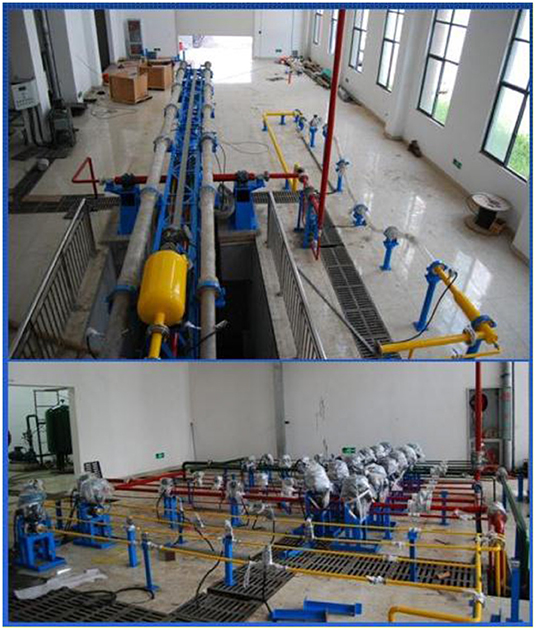
Figure 1. Photos of experimental setup at Yangtze University.

TABLE 1

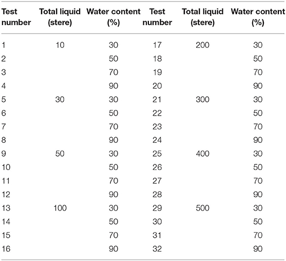
Table 1. Measured liquid volume and water cut of oil–water two-phase flow experiments.

The fluids utilized in the experiments include diesel (with a light brown color), tap water, and air. The density and viscosity of diesel oil are, respectively, at standard temperature and pressure. A Newtonian fluid flow behavior is displayed (Xu et al., 2020). The density and viscosity of tap water is 0.9884 g/cm³ and 1.16 mPa·s at standard temperature and pressure, respectively (Pang et al., 2020). The air density is 0.001223 g/cm³ at standard temperature and pressure (Vollestad et al., 2020). Table 1 lists the experimental measurements of total liquid and water cut for each test.

A simulation wellbore and bench are used with the experimental equipment as shown in Figure 1. The simulated wellbore is 159 mm (7 inches) in diameter and 124 mm (5.5 inches) in diameter. The simulated well in the laboratory is 12 m long, and there are 10-m transparent wells in the middle. Each section of the transparent well is 2 m long, and there are 1-m stainless steel wells at both ends of the well. The center distance between the two shafts is 800 mm, and the bottom of the shaft and the height of 5 m are equipped with a gas–liquid mixer. Three pressure sensors and three temperature sensors are arranged uniformly from top to bottom in each wellbore, and they are used to measure the pressure and temperature changes in the wellbore simulated by glass. The procedures for each experimental test can be described as follows: (1) design the ratio of different phases based on data listed in Table 1, (2) fill up the fluids in the experiment platform, (3) run the equipment through a computer controlling system, (4) observe transformations of flow pattern directly through the transparent glass pipe and capture the images (as shown in Figure 2) of such transformations by a digital camera. The flow rates of oil, gas, and water in the experiments are specifically designed according to field data. The experimental oil–water distribution is shown in Table 1. Under the current circumstances, the oil–water flow is a common flow pattern. The images of the gas–water two- and three-phase flow are captured during the tests. The experiment is conducted at standard temperature and pressure. Specifically, a transparent glass pipe with an inner diameter of 124 mm and length of 5.2 m is installed for visual observation of fluid morphology within the flow line (Feng et al., 2017).

FIGURE 2

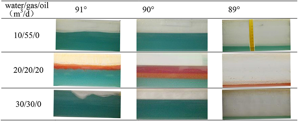
Figure 2. Experimental Images of the Multiphase Flow within a Horizontal Well.

The experimental platform consists of an orientation-adjustable pipeline, which can be adjusted with an angle from vertical (0°) to horizontal (90°) so that multiphase fluid flow analyses based on various angles can be conducted within this pipe. In the meantime, the fluid phase transmission can be directly observed from the translucent pipeline. Figure 2 shows the captured images of a flow pattern of the multiphase flow.

As shown in Figure 2, different angles represent different orientations of the pipeline, e.g., 89° and 91°, respectively, mean an upswept pipeline and a sloping-down pipeline, and 90° indicates that the pipeline is in a standard horizontal direction. We can take pictures of two- and three-phase flow. For a fixed proportion of fluid mixtures with a low flow volume as shown in experiments 1–12 in Table 1, a tiny change of angle (e.g., 1°) could lead to a significant variation of the flow pattern. More specifically, at 90°, the fluid pattern is laminar with a flat fluid interface (i.e., water–gas, water–oil, and oil–gas) that can be clearly observed; however, the interface becomes more indistinct and uneven when the tilt angle changes to 91° or 89°. It appears to be a mixed color when the tilt angle changes for different zones' flow volume. It is also observed from the experiments that, for a system with a fixed fluid proportion, no change of flow pattern can be observed if the tilt angle stays unchanged.

The Production Profile Interpretation Model

In practice, a real horizontal well is not absolutely horizontal in that a certain fluctuation exists on the well trajectory of the production section as shown in Figure 3. As demonstrated in Figure 2, when the tilt angle changes, the flow pattern also changes without the flow volume, velocity, and phase fraction of each component kept the same. Based on this observation, a calculation model using the same tilt angle is presented to calculate the fluid distribution profile of each phase by utilizing the optimized method. The same tilt angle is at A1 and A2 or B1 and B2 as shown in Figure 3. This is the interpretation model for the production profile on the same angle of the horizontal well trajectory. By using this methodology, we can design a model to calculate the value of the production layer. The differences among the different layers are used to calculate the production of each interpretation layer.

FIGURE 3

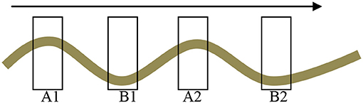
Figure 3. Division of Interpretation Layer of Horizontal Well.

The calculation model is summarized below. In Figure 3, the oil, gas, and water are flowing simultaneously from left to right. The wave line in Figure 3 is the horizontal well trajectory. The rightward direction of the arrow indicates the flow direction. First, the production value of each interpretation layer is calculated according to the marked signs (i.e., A1, A2, B1, B2) in the graph; all these layers are horizontal (i.e., 90°), and the flow patterns are laminar as indicated in Figure 2. Then, the flow difference between every interval is calculated.

$\begin{array}{ll}\begin{array}{c}{\Delta }_1=Q_{A2}-Q_{A1}\\ {\Delta }_2=Q_{B2}-Q_{B1}\end{array}& (1)\end{array}$

where Q_A1, Q_A2, Q_B1, and Q_B2 are the production value of each layer; Δ₁ is the production value of Q_A2 minus Q_A1; and Δ₂ is the production value of Q_B2 minus Q_B1.

Three interpretations for the calculated values of Δ are presented as follows: (1) Δ = 0 means there is no production value between these two layers, (2) Δ > 0 means production exists with a value of Δ between those two layers, and (3) Δ < 0 means there is a suction value of the layer. In this way, the producing layer can be identified, and the production rate of each layer can be calculated more precisely.

According to the formula (1) of the multiphase production Q, the key point of the interpretation methods is to precisely calculate the apparent velocity of fluid (Va) and the velocity correction factor (Cv) (Zeng and Yao, 2020). The Va can be determined from the measurement of turbine flow velocity, tracer measurement, etc. Va value is a relied-upon measurement (China University of Petroleum-Beijing, 2020). The Va value method depends on the difference in the measuring instrument. For example, in turbine flow measurement, Va is obtained by turbine measures. In tracer flow measurement, Va value is the tracer measurement value.

The new interpretation method proposes a back calculation to generate the value of Va. The formula is as follows: Va = Q/Cv × Pc. In this formula, Q represents the set-point value of the production layer, Cv is the fluid velocity profile correction factor, and Pc is the pipe diameter constant. If the correct Cv value is utilized, the calculated Va is equal to the measured value, which indicates that the correct production value of Q is achieved. If the calculated Va is not matched with the experimental data, the value of Q is optimized until matching is achieved.

In order to calculate Cv, several important parameters, such as the inner diameters of casing pipes (D, unit: m), mean velocity of fluid (Vm, unit: m/s), fluid density (unit: kg/m3), and fluid viscosity (unit: mPa·s), are calculated. Furthermore, the Reynolds number is calculated, and the corresponding Cv value is determined by using the interpolation algorithm.

Upon completion of the aforementioned calculations, the production value of each fluid phase, Q (where Q is the calculation value; the previous Q is a set-point value), can be calculated. Upon completion of the calculation of Q, the output of every interpretation layer can be determined.

Design of the Calculation Principle

For this study, an algorithm that is designed to automatically recognize the true slope angle of the horizontal well trajectory was developed. The slope angle is according to the same tilt angle value, and the same tilt angle value directly affects the interpretation accuracy of the model. At the same tilt angle, the design scheme to calculate the production value of each phase of the horizontal well is shown in Figure 4. The values of Qw, Qo, and Qg were calculated by using the respective fluid physical properties, velocity profile correction factor, and tilt angle interpretation model. The process includes the inversion calculations of oil, gas, and water phase holdup, flow velocity, density, and apparent flow velocity contour. These values can be obtained from measuring production data. The flow pattern includes both the laminar and turbulent flow.

FIGURE 4

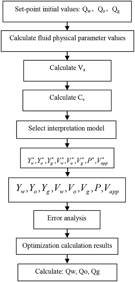
Figure 4. Calculation model of corotating angle of multiphase flow.

The water/oil/gas holdup represents the fraction of the flowing volume of water/oil/gas with respect to the total volume of the pipe per unit length. In Figure 4, the Qw is initially the set-point water value of the producing layer, Qo is initially the set-point oil value of the producing layer, and Qg is initially the set-point gas value of the producing layer. The water, oil, and gas holdup is Yw^*, Yo^*, and Yg^*, respectively. The water, oil, and gas flow rate is Vw^*, Vo^*, and Vg^*. The flow density is P^*, and the apparent fluid velocity is Vapp^*. They are all calculated from the inversion method in formula (2) to formula (11). In Figure 4, the water, oil, and gas holdup is Yw (Yw is measured by an instrument), Yo (Yo is measured by an instrument), and Yg (Yg is measured by an instrument), respectively. Water, oil, and gas flow rates are Vw (Vw is measured by an instrument), Vo (Vo is measured by an instrument), and Vg (Vg is measured by an instrument). The flow density is P (P is measured by an instrument), and the apparent fluid velocity is Vapp (Vapp is measured by an instrument). The values for each variable are initially assumed and then the values are calculated and compared with the measured data. If the retrieved calculation data are consistent with the measured values, the results of the inversion calculation are treated as accurate. The initial production values for the water, oil, and gas phases (Qw, Qo, Qg) of the interpretation layer are established, and the value of each phase is optimized until the calculated value and the measured data are matched. The key point is to design the same-angle calculation model or a related algorithm through the analysis of the relevant experimental data.

A calculation model of the production logging profile under the same tilt angle is developed, and the specific process is presented below.

In step 1, the horizontal well track is drawn, the near horizontal level is found qualitatively according to the track, and the interpretation of each layer is determined for different tilt angles.

In step 2, an initial production value for the whole zone flow layer is assumed. The mean fluid velocity of each phase of the well is calculated, and the production value is the flow value within the well. The Va is calculated according to the relationship between the Reynolds number and the velocity profile, and then the value of apparent velocity of fluid is determined.

In step 3, the drift and slip velocities are calculated according to the drift and slip models. Then, the value of each water holdup for each layer is calculated. If the calculated value is the same as the practical value, the assumed initial total production value should be consistent with the practical production value. If not, the calculated holdup value is used as a known parameter for further calculation. Then, the initial production value is reset, and the value of each water holdup is recalculated. Next, repeat steps 1 and 2.

In step 4, the value of flow velocity of each phase is calculated after the water holdup. If the velocity stays the same as the practical value, the density value of each phase is calculated. Otherwise, the initial production value is reset, and the water holdup and flow velocity values are recalculated. Repeat steps 3 and 4 until the holdup value and the density value of each phase match the practical value.

In step 5, based on the correct holdup and flow velocity values, the density value is calculated. If the calculated density value is the same as the practical value, cease the calculation process. If not, reset the initial production value and repeat steps 2–5 until the values of the water holdup, flow velocity, and density are similar to the practical values. Then the process is terminated, and the values are finalized, which includes mean flow velocity, apparent velocity, slip velocity, drift velocity, water holdup, fluid velocity, and fluid density.

In step 6, based on the calculated parameters from the expert fluid property database and combined with the values from step 5, the flow value (the flow can mean flux) of each phase is calculated by decreasing the whole flow layer by layer.

The method is demonstrated by using the water–oil case as an example. The interpretation model for the production profile on the same angle of horizontal well trajectory is used to calculate the whole flow layer production, average flow velocity, apparent velocity, slip velocity, drift velocity, water holdup of each phase, each phase's fluid velocity, and fluid density.

According to the well track, the initial values (Q_o, Q_w, unit per day) of the oil and gas phase flows are set on the full flow layer, the apparent flow velocity (V_a, unit m/min), the slip velocity (V_s, unit m/min), the oil holdup Y_o, water holdup Y_w, actual flow velocity of oil (V_o, unit m/min), and the actual flow velocity of water (V_w, unit m/min); the other data are the pipe diameter constant (P_c, (m³/d)/(m/min)), the external diameter (D, unit mm), the density of water (ρ_w, unit g/cm³), the density of oil (ρ_o, unit g/cm³), which are determined by using the inversion optimization method.

Formula (2) is used to calculate the pipe diameter constant.

$\begin{array}{ll}{P}_c=\frac{1}{4}\pi D^2\times 60\times 24\times {10}^{-6}& (2)\end{array}$

Then formula (3) is used to calculate the mean fluid velocity.

$\begin{array}{ll}{V}_m=\frac{Q_o+Q_w}{P_c}& (3)\end{array}$

After that, according to the initial values of Q_o and Q_w, by combining the expert knowledge database and the fluid-producing profile by using the method of optimized iteration computation, the value of Cv is obtained. Formula (4) is used to calculate the apparent fluid velocity Va, and formulas (5) and (6) are used to calculate the superficial velocity of the oil and gas. The relationship is that Cv multiplied by Va makes the velocity profile (Vm).

$\begin{array}{ll}{v}_a=\frac{v_m}{C_v},& (4)\end{array}$

$\begin{array}{ll}{v}_{so}=\frac{Q_o}{P_c},& (5)\end{array}$

$\begin{array}{ll}{v}_{sw}=\frac{Q_w}{P_c}.& (6)\end{array}$

Combine the known parameters v_so, v_sw, v_m, ρ_w, ρ_o, θ, and formulas (7) and (8) to calculate the values of v_s and Y_w.

$\begin{array}{l}{v}_s=12.013{({\rho }_w-{\rho }_o)}^{{}^1{/}_4}exp[-0.788(1-Y_w)ln\frac{1.85}{{\rho }_w-{\rho }_o}]\\ (1+0.04*\theta ),& (7)\end{array}$

$\begin{array}{ll}{V}_{so}=(1-Y_w)V_m+Y_w(1-Y_w)V_s.& (8)\end{array}$

In formula (7), the density values of water and oil are obtained from the expert database, and θ is the tilt angle of the horizontal well (unit °). The oil holdup can be calculated by using formula (9).

$\begin{array}{ll}{Y}_o=1-Y_w,& (9)\end{array}$

$\begin{array}{ll}{V}_o=\frac{V_{so}}{1-Y_w}=\frac{Q_o}{P_c(1-Y_w)},& (10)\end{array}$

$\begin{array}{ll}{V}_w=\frac{V_{sw}}{Y_w}=\frac{Q_w}{P_c{Y}_w}.& (11)\end{array}$

Finally, formulas (9) and (10) are used to calculate the actual velocity of oil and water. The density also can be found from using a measuring tool to measure.

By comparing the data obtained from the inversion method and the measured value, the initial production values of oil and water are determined to be correct or not. If the data from the inversion analogy are similar to those of the measured values, the production value is the target value. Otherwise, the production value is optimized.

The production profile Q_A1, Q_A2, Q_B1, and Q_B2 values of the horizontal well are compared with those data generated by using formula (1) to obtain the difference between tilt angles Δ₁, Δ₂ values for the purpose of finding the productive interval and the corresponding parameters.

Precise Verification of the Interpretation Result

In order to verify the rationality of the interpretation results, a total of five horizontal wells' production logging data were analyzed, and the interpretation results were further compared with the actual measured values. Table 2 shows the difference of the single-phase flow between the interpretation results and the measured data by using the logging tool. The measured data were calculated by using the model to get the interpretation values. The model is the interpretation model for the production profile on the same angle of the horizontal well trajectory.

TABLE 2

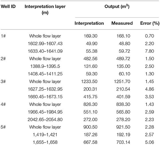
Table 2. Comparison of interpreted single-phase flow with the measured data.

Table 2 shows that for the actual measured data in the wellhead area, the maximum and minimum errors of layer flow are 7.8 and 0.7%, respectively. The error is the difference between the measured data and the interpreted values divided by the measured value.

Table 3 shows that the maximum error of the simulated result is 9.8% in a three-phase flow horizontal well, and the maximum error of the two-phase flow is 0.5%.

TABLE 3

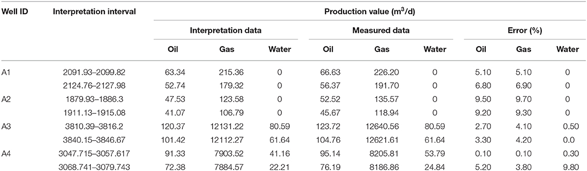
Table 3. Comparison of interpreted wellhead multiphase flow results with measured data.

Conclusions

In this paper, a multiphase flow pattern mechanism for a horizontal well is studied and analyzed by a proposed calculation methodology that uses the same tilt angle for a highly deviated well. The main innovation point of this research is the interpretation method with the same tilt angle. The production logging interpretation method and the model proposed in this paper are only applicable to the production logging interpretation of a single well and not applicable for cluster wells.

The change of the tilt angle has great influence on the flow pattern when the flow rate is low. Thus, an interpretation method for calculating the production profile with the same tilt angle was developed. The algorithm flow chart of the interpretation model was constructed and the relevant algorithm model and formula was deduced based on the two-phase example. This study designs an inclined angle interpretation method by studying the horizontal flow pattern. Furthermore, it leads to the development of a series of interpretation models for production logging of a horizontal well by studying relevant calculation methods and models. Therefore, interpretation accuracy of horizontal wells is significantly improved. Further study will be focused on the study for multiphase flow and improvement of the current calculation model.

Data Availability Statement

All datasets generated for this study are included in the article/supplementary material.

Author Contributions

WS: conceptualization, funding acquisition, investigation, and writing—original draft. NJ and WS: data curation and writing—review and editing. QJ: formal analysis, methodology, project administration, resources, software, supervision, validation, and visualization. All authors contributed to the article and approved the submitted version.

Conflict of Interest

The authors declare that the research was conducted in the absence of any commercial or financial relationships that could be construed as a potential conflict of interest.

Acknowledgments

The author would like to thank the support received from Xinjiang Uygur Autonomous Region Innovation Environment (talent, base) Construction Foundation (Xinjiang NSFC Program Foundation 2020D01A132): Research and implementation of horizontal well inversion optimization interpretation method. Jingzhou Science Technology Foundation (2019EC61-06) and Hubei Science and Technology Demonstration Foundation (2019ZYYD016).

References

China University of Petroleum-Beijing (2020). Patent Issued for Apparatus for Physical Simulation Experiment for Fracturing in Horizontal Well Layer by Layer by Spiral Perforation and Method (USPTO 10,550,688). Electronics Newsweekly.

Google Scholar

Feng, Q., Xia, T., Wang, S., and Singh, H. (2017). Geofluids; research institute of petroleum exploration and development researchers report recent findings in geofluids (transient pressure analysis for multifractured horizontal well with the use of multilinear flow model in shale gas reservoir). Sci. Lett. 111–117.

Google Scholar

Hayati-Jafarbeigi, S., Mosharaf-Dehkordi, M., Ziaei-Rad, M., and Dejam, M. (2020). A three-dimensional coupled well-reservoir flow model for determination of horizontal well characteristics. J Hydrol. 585:124805. doi: 10.1016/j.jhydrol.2020.124805

CrossRef Full Text | Google Scholar

Ji, B. (2012). Progress and prospects of enhanced oil recovery technologies at home and abroad. Oil Gas Geol. 33,111–117.

Google Scholar

Jinghong, H., Ruofan, S., and Yuan, Z. (2020). Investigating the horizontal well performance under the combination of micro-fractures and dynamic capillary pressure in tight oil reservoirs. Fuel 269:117375. doi: 10.1016/j.fuel.2020.117375

CrossRef Full Text | Google Scholar

Keles, C., Tang, X., Schlosser, C., Louk, A. K., and Ripepi, N. S. (2020). Sensitivity and history match analysis of a carbon dioxide “huff-and-puff” injection test in a horizontal shale gas well in Tennessee. J. Nat. Gas Sci. Eng. 77:103226. doi: 10.1016/j.jngse.2020.103226

CrossRef Full Text | Google Scholar

Li, G., Qin, Y., Liu, L., He, Q., Chen, F., and Zhang, Y. (2013). Application of overall fracturing technology for cluster horizontal wells to the development of low permeability tight gas reservoirs in the Daniudi Gas Field, Ordos Basin. Nat. Gas Industry 33, 49–53.

Google Scholar

Li, H., Tan, Y., Jiang, B., Wang, Y., and Zhang, N. (2018). A semi-analytical model for predicting inflow profile of horizontal wells in bottom-water gas reservoir. J. Petrol. Sci. Eng. 160, 351–362. doi: 10.1016/j.petrol.2017.10.067

CrossRef Full Text | Google Scholar

Lian, L., Qin, J., Yang, S., Yang, Y., and Li, Y. (2013). Analysis and evaluation on horizontal well seepage models and their developing trends. Oil Gas Geol. 34, 821–827. doi: 10.11743/ogg20130616

CrossRef Full Text

Lian, Z., Zhang, Y., Zhao, X., Ding, S., and Lin, T. (2015). Establishment and application of mechanical and mathematical models for multi-stage fracturing strings in a horizontal well. Nat. Gas Industry 35, 85–91.

Google Scholar

Liu, S., Zhu, Z., and Balint, S. (2020). Application of composite deflecting model in horizontal well drilling. Hindawi 2020:4672738. doi: 10.1155/2020/4672738

CrossRef Full Text | Google Scholar

Lum, J. Y. L., Lovick, J., and Angeli, P. (2004). Dual continuous horizontal and low inclination two-phase liquid flows. Canad. J. Chem. Eng. 83, 303–315. doi: 10.1002/cjce.5450820211

CrossRef Full Text | Google Scholar

Luo, H., Li, H., Lu, Y., and Zhenhua, G. (2020a). Inversion of distributed temperature measurements to interpret the flow profile for a multistage fractured horizontal well in low-permeability gas reservoir. Appl. Math. Model. 77, 360–377. doi: 10.1016/j.apm.2019.07.047

CrossRef Full Text | Google Scholar

Luo, H., Li, H., Tan, Y., Li, Y., Jiang, B., Lu, Y., et al. (2020b). A novel inversion approach for fracture parameters and inflow rates diagnosis in multistage fractured horizontal wells. J. Petrol. Sci. Eng. 184:106585. doi: 10.1016/j.petrol.2019.106585

CrossRef Full Text | Google Scholar

Luo, W., Li, H., Wang, Y., and Wang, J. C. (2015). A new semi-analytical model for predicting the performance of horizontal wells completed by inflow control devices in bottom-water reservoirs. J. Nat. Gas Sci. Eng. 27, 1328–1339. doi: 10.1016/j.jngse.2015.03.001

CrossRef Full Text | Google Scholar

Pang, Z., Jiang, Y., Wang, B., Cheng, G., and Yu, X. (2020). Experiments and analysis on development methods for horizontal well cyclic steam stimulation in heavy oil reservoir with edge water. J. Petrol. Sci Eng. 188:106948. doi: 10.1016/j.petrol.2020.106948

CrossRef Full Text | Google Scholar

Song, W., Jiang, Q., Li, J., and Li, M. (2015). Equal-tilt-angle production profile calculation model of horizontal wells. Oil Gas Geol. 36, 688–694.

Google Scholar

Tan, Y., Li, H., Zhou, X., Wang, K., Jiang, B., and Zhang, N. (2019). Inflow characteristics of horizontal wells in sulfur gas reservoirs: a comprehensive experimental investigation. Fuel 238, 267–274. doi: 10.1016/j.fuel.2018.10.097

CrossRef Full Text | Google Scholar

Tang, Q. (2013). Application of geosteering technology in the developent of Sulige gas field—case studies of the Su10 and Su53 blocks. Oil Gas Geol. 34, 388–393. doi: 10.11743/ogg20130316

CrossRef Full Text | Google Scholar

Tian, Q., Cui, Y., Luo, W., Liu, P., and Ning, B. (2020). Transient flow of a horizontal well with multiple fracture wings in coalbed methane reservoirs. Energies 13:1498. doi: 10.3390/en13061498

CrossRef Full Text | Google Scholar

Tian, Z., Shi, L., and Qiao, L. (2015). Research of and countermeasure for wellbore integrity of shale gas horizontal well. Nat. Gas Industry 35, 70–76. doi: 10.3787/j.issn.1000-0976.2015.09.010

CrossRef Full Text | Google Scholar

Vollestad, P., Angheluta, L., and Jensen, A. (2020). Experimental study of secondary flows above rough and flat interfaces in horizontal gas-liquid pipe flow. Int. J. Multiphase Flow 125:103235. doi: 10.1016/j.ijmultiphaseflow.2020.103235

CrossRef Full Text | Google Scholar

Wang, X., Yu, G., and Li, Z. (2006). Productivity of horizontal wells with complex branches. Petrol. Explor. Dev. 33, 729–733.

Google Scholar

Wu, Z., Dong, L., Cui, C., Cheng, X., and Wang, Z. (2020). A numerical model for fractured horizontal well and production characteristics: comprehensive consideration of the fracturing fluid injection and flowback. J. Petrol. Sci. Eng. 187:106765. doi: 10.1016/j.petrol.2019.106765

CrossRef Full Text | Google Scholar

Xie, D., Huang, Z., Ma, Y., Vaziri, V., Kapitaniak, M., and Wiercigroch, M. (2020). Nonlinear dynamics of lump mass model of drill-string in horizontal well. Int. J. Mech. Sci. 174:105450. doi: 10.1016/j.ijmecsci.2020.105450

CrossRef Full Text | Google Scholar

Xu, J., Dong, N., Zhu, C., Liu, J., and Chen, T. (2012). Application of seismic data to the design of horizontal well trajectory in tight sandstone reservoirs. Oil Gas Geol. 33, 909–913.

Google Scholar

Xu, Y., Li, X., and Liu, Q. (2020). Pressure performance of multi-stage fractured horizontal well with stimulated reservoir volume and irregular fractures distribution in shale gas reservoirs. J. Nat. Gas Sci. Eng. 77:103209. doi: 10.1016/j.jngse.2020.103209

CrossRef Full Text | Google Scholar

Yue, M., Zhang, Q., Zhu, W., Zhang, L., Song, H., and Li, J. (2020). Effects of proppant distribution in fracture networks on horizontal well performance. J. Petrol. Sci. Eng. 187:106816. doi: 10.1016/j.petrol.2019.106816

CrossRef Full Text | Google Scholar

Yue, P., Du, Z, Chen, X., Zhu, S. Y., and Jia, H. (2015). Critical parameters of horizontal well influenced by semi-permeable barrier in bottom water reservoir. J. Central South Univer. 22, 1448–1455. doi: 10.1007/s11771-015-2662-z

CrossRef Full Text | Google Scholar

Zeng, Q., and Yao, J. (2020). Production calculation of multi-cluster fractured horizontal well accounting for stress shadow effect. Int. J. Oil Gas Coal Tech. 23:293. doi: 10.1504/IJOGCT.2020.105773

CrossRef Full Text | Google Scholar

Zhai, L., Jin, N., and Zheng, X. (2012). The analysis and modeling of measuring data acquired by using combination production logging tool in horizontal simulation well. Chin. J. Geophys. 55, 1411–1421. doi: 10.6038/j.issn.0001-5733.2012.04.037

CrossRef Full Text | Google Scholar

Zong, Y. (2009). Measurement of the Properties of Oil-Water Two-Phase Flow in Inclined and Horizontal Pipes. Tianjin: Tianjin University.

Google Scholar