Simultaneous Cycle Optimization and Fluid Selection for ORC Systems Accounting for the Effect of the Operating Conditions on Turbine Efficiency

The design of optimal organic Rankine cycle (ORC) systems requires the simultaneous identification of the optimal cycle architecture, operating conditions and working fluid, whilst accounting for the effect of these parameters on expander performance. In this paper, a novel method for predicting the design-point efficiency of a radial turbine is developed, which can predict the achievable efficiency based only on the thermodynamic conditions. This model is integrated into an optimization framework in which the working fluid is modeled using the Peng-Robinson equation of state and the fluid parameters (i.e., critical temperature) are simultaneously optimized alongside the cycle conditions. This framework can evaluate recuperated and transcritical cycles, whilst heat-transfer area requirements are estimated based on representative overall heat-transfer coefficients. For a range of heat sources, a single-objective optimization is first completed in which power output is maximized, which is then followed by a multi-objective optimization in which the trade-off between power output and total heat-transfer area is investigated. It is demonstrated that the optimization framework can simultaneously optimize the working fluid and cycle parameters, and identify whether a subcritical or transcritical cycle, with or without a recuperator, is best suited for a particular application, whilst accounting for the effect of these variables on the expander performance. This information is critical to identify optimal cycle configurations and working fluids that result in the best thermodynamic performance, yet exist in the design space in which feasible turbines can be designed. It is found that the optimal critical temperature does not vary significantly between different cycle architectures, and is not affected by whether a single or multi-objective optimization is completed. However, including the expander performance model results in significantly different cycles to optimal thermodynamic cycles.

1. Introduction

The use of organic Rankine cycle (ORC) technology to covert low-temperature heat (< 400°C) is widely studied (Imran et al., 2018), and the number of plants installed globally continues to grow (Tartière and Astolfi, 2017). However, challenges including high investment costs, and the lack of suitable components at the smaller scale mean the penetration of ORC technology into domestic and commercial-scale applications remains limited. Hence, interest in improving the performance, both from a technical and economic perspective, alongside the development of new expander designs remain pertinent research areas.

The identification of optimal thermodynamic cycles and working fluids for ORC systems has been studied in detail. These studies are numerous, and hence only a few notable studies are referred to here. The simplest of these involve a parametric optimization study in which a range of fluids are evaluated by comparing optimal cycles that maximize thermodynamic performance, such as power output or overall energy efficiency (Saleh et al., 2007; Schwoebel et al., 2017). These studies assume fixed component efficiencies and only consider thermodynamic performance. The next step is to integrate thermodynamic analysis with heat-exchanger sizing models, enabling the trade-off between performance and heat-transfer area to be investigated. Subsequently, the implementation of component cost correlations enables the trade-off between thermodynamic and economic performance to be investigated through multi-objective optimization (Quoilin et al., 2011; Lecompte et al., 2013; Pierobon et al., 2013; Andreasen et al., 2016; Oyewunmi and Markides, 2016).

Despite the increasing complexity of these models, most studies either consider a pre-prescribed fluid or apply the same optimization model to a group of fluids. However, the next generation of models integrate fluid selection with cycle optimization by introducing fluid parameters that describe the molecular structure of the fluid into the optimization process. Computer-aided molecular and process design (CAMPD) models are capable of combining the entire process into a single optimization, and of identifying fluid candidates that may otherwise be overlooked. The studies by Papadopoulos et al. (2010, 2013) were the first to apply this method to ORC system design, using it to identify optimal fluids based on thermodynamic performance, cost, toxicity and flammability. Later, Palma-Flores et al. (2016) identified fluids based on thermodynamic performance and safety characteristics, whilst Cignitti et al. (2017) considered heat-exchanger requirements alongside thermodynamic performance. All of these studies, alongside those by Brignoli and Brown (2015) and Su et al. (2017b) use cubic equations of state, such as the Peng-Robinson (Peng and Robinson, 1976) or Redlich-Kwong-Soave (Soave, 1972) models. Alternatively, more sophisticated equations of state, based on statistical-associating fluid theory (Chapman et al., 1990) have also been used. Research at RWTH Aachen University has developed ORC-CAMPD models based on the PC-SAFT equation of state (Lampe et al., 2014, 2015; Schilling et al., 2016, 2017), whilst research at Imperial College London has developed similar models based on the SAFT-γ Mie equation of state (Oyewunmi et al., 2016; White et al., 2017, 2018; van Kleef et al., 2018). Within both research groups, their latest research focussed on integrating heat-exchanger sizing models into the CAMPD model, thus facilitating optimal fluids and cycles to be identified based on economic performance indicators.

Another important consideration is the effect of the cycle operating conditions on expander performance. Optimal thermodynamic cycles typically require large volumetric expansion ratios, which have implications for expander design. For large-scale applications a multi-stage axial turbine is generally favored. However, for small-scale applications a single-stage expander is preferred. Volumetric expanders are suitable for low expansion ratios, whilst turbo-expanders are suitable for a larger range of expansion ratios. Furthermore, for low mass-flow rates radial turbines are preferred over their axial counterparts. Thus, radial turbines are the presumed expander technology within this work. However, even then, their performance is subject to the operating conditions, with high expansion ratios corresponding to small rotor-inlet blade heights and supersonic conditions within the turbine. Therefore, expander performance should be accounted for within cycle optimization studies. This involves developing mean-line turbine design and performance models, integrating these with thermodynamic cycle models, and completing the optimization of both turbine and cycle simultaneously. For a radial turbine, this typically involves optimizing six turbine design parameters, alongside the working fluid and cycle parameters. Examples of such studies include those by Bahamonde et al. (2017) and Meroni et al. (2018). However, the major disadvantage of these studies, particularly for preliminary sizing, is the complexity of the resulting model and optimization problem. Alternatively, non-dimensional parameters (i.e., specific-speed, specific-diameter and size parameter) are widely used to estimate the diameter and rotational speed required for a particular turbine to obtain a high efficiency. These methods rely heavily on empirical data for turboexpanders operating with ideal gases, although there have been important studies correlating these parameters against efficiency for single- and multi-stage ORC axial turbines (Macchi and Perdichizzi, 1981; Astolfi and Macchi, 2015). Whilst there have been attempts to develop similar maps for ORC radial turbines (Perdichizzi and Lozza, 1987; Lio et al., 2017; Mounier et al., 2018), these methods remain unvalidated, and to the authors' knowledge, have not been rigorously integrated within cycle optimization studies. Thus, there remains a need to develop methods to predict turbine efficiency without requiring more detailed expander performance models.

To improve the performance of ORC systems, alternative cycle architectures have been proposed, such as transcritical cycles (Chen et al., 2010), cycles operating with two-phase expansion (Fischer, 2011), and cycles operating with a fluid mixture (Angelino and Colonna, 1998). The intention behind these cycles is to completely, or partially, remove the isothermal heat-addition heat-transfer process into the system, thus reducing irreversibility and improving thermodynamic performance. However, in each case the reduced irreversibility does come at the cost of larger heat exchangers, whilst the three cycles are associated with higher operating pressures, a lack of suitable two-phase expanders, particular for high volume ratios, and detrimental heat-transfer properties, respectively. Thus, ORC optimization studies should account for different cycle architectures and consider these trade-offs.

The aim of this study is to combine these aforementioned aspects into a single framework. The framework is similar to ORC-CAMPD models in that it can simultaneously optimize key fluid parameters alongside the cycle operating conditions, based on both single and multiple objective functions. However, this study goes beyond previous studies by introducing a novel expander model that accounts for the effects of the working fluid and operating conditions on the expander performance, and by considering transcritical cycles. This allows a group of systems to be identified for a given application that optimally capture the trade-off between thermodynamic performance and heat-exchanger area, yet exist in a design space in which feasible turboexpanders can be designed. The first main novelty lies in the development of the new method for predicting the design-point efficiency of a radial turbine based only on thermodynamic conditions. The second lies in the completion of a multi-objective optimization of the fluid and cycle parameters for subcritical and transcritical cycles, with or without recuperation, accounting for expander performance. It is found that the optimal critical temperature does not vary significantly between different cycle architectures, and is not affected by whether a single or multi-objective optimization is completed. However, including the expander performance model results in significantly different cycles to optimal thermodynamic cycles. These results help to identify general relationships that can streamline fluid and cycle selection in the future. Following this introduction, a description of the developed model is provided in section 2. Then, in section 3, a case study is defined for which a group of single- and multi-objective optimization studies are completed. The results are presented and discussed in section 4, and the conclusions from this study are summarized in section 5.

2. System and Component Modeling

2.1. Peng-Robinson Equation of State

Within this work the cubic Peng-Robinson equation of state is used to model the working fluid (Peng and Robinson, 1976), which allows a potential fluid to be defined in a more generalized way than using more sophisticated models, such as REFPROP (Lemmon et al., 2013), which, in turn, allows the working fluid to become a variable within the optimization process. The precise details on how the Peng-Robinson model is implemented within the ORC model are described in White and Sayma (2018), but in summary, the Peng-Robinson equation state is defined as:

$\begin{array}{ll}p=\frac{RT}{V_{\text{m}}-b}-\frac{a\alpha (T)}{V_{\text{m}}^2+2b{V}_{\text{m}}-b^2},& (1)\end{array}$

where p is the pressure in Pa, R is the universal gas constant with units J/(mol K), T is the temperature in K, and V_m is the molar volume with units of m³/mol. The parameters a and b, and the function α(T), are fluid-specific and are functions of the critical temperature T_cr, critical pressure p_cr, and acentric factor ω. Alongside Equation (1) a second-order polynomial is used to model the ideal-gas specific-heat capacity:

$\begin{array}{ll}{c}_{p,\text{id}}(T)=A+BT+C{T}^2,& (2)\end{array}$

where the coefficients A, B, and C are constants that control the shape of the fluid's saturation dome, and thus whether the fluid has a saturated vapor line with a positive or negative gradient and is categorized as dry or wet, respectively. This has been demonstrated in our previous study (White and Sayma, 2018).

Using Equations (1, 2) all of the required properties to analyse the thermodynamic cycle, namely the specific enthalpy h in J/mol, the specific entropy s in J/(mol K), and the specific volume v = 1/ρ in m³/mol, can be determined based on a vector of six fluid parameters:

$\begin{array}{ll}\text{x}=\left[T_{\text{cr}},p_{\text{cr}},\omega ,A,B,C\right].& (3)\end{array}$

2.2. Thermodynamic ORC Model

The thermodynamic ORC model described in the same previous study (White and Sayma, 2018) is used here, although a number of modifications have been implemented. To summarize, the cycle is assumed to operate under a steady-state, and no heat losses or pressure drops are considered. The heat-source and heat-sink are defined by an inlet temperature, mass-flow rate, and temperature independent specific-heat capacity. The ORC state points are defined by: the condensation temperature T₁; the evaporation reduced pressure p_r, defined as ratio of the evaporation pressure to the critical pressure, i.e., p_r = p₂/p_cr; and the amount of superheat ΔT_sh. The pump is modeled with a fixed isentropic efficiency η_p, whilst the turbine is modeled using a new variable efficiency turbine model, described in section 2.3. A schematic of the ORC system under consideration is provided in Figure 1.

FIGURE 1

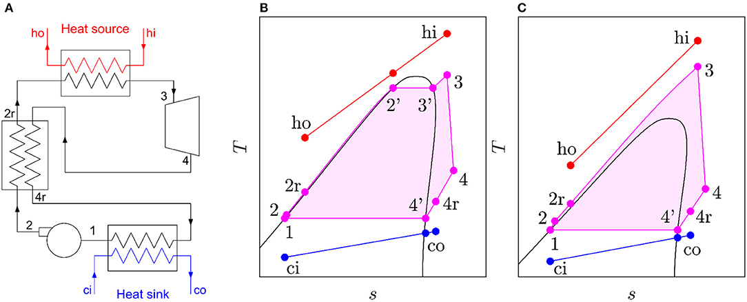
Figure 1. Description of the ORC systems considered within this study: (A) schematic of a recuperated ORC system; (B) T-s diagram of a subcritical recuperated ORC system; and (C) T-s diagram of a transcritical recuperated ORC system.

Within this current study the model has been adapted to also evaluate transcritical and recuperated cycles. The former is achieved by allowing p_r to exceed unity, and then defining ΔT_sh as:

$\begin{array}{ll}\Delta T_{\text{sh}}=\{\begin{array}{ll}{T}_3-T_{3^{\prime }}\hfill & \text{if }{p}_r<1\hfill \\ T_3-T_{\text{cr}}\hfill & \text{otherwise},\hfill \end{array}& (4)\end{array}$

where T₃ is the turbine inlet temperature and $T_{3^{\prime }}$ is the saturation temperature. Moreover, because there is no distinct location for the evaporator pinch-point in a transcritical cycle, the non-dimensional heat-source temperature drop is defined as:

$\begin{array}{ll}\theta =\frac{T_{\text{hi}}-T_{\text{ho}}}{T_{\text{hi}}-T_{\text{ci}}},& (5)\end{array}$

where T_hi and T_ci are the heat-source and heat-sink inlet temperatures and T_ho is the heat-source outlet temperature. Specifying θ, in turn, defines the ORC working-fluid mass-flow rate. The recuperator effectiveness is introduced as the last cycle variable, defined as:

$\begin{array}{ll}\epsilon =\frac{h_{2\text{r}}-h_2}{\Delta h_{\text{max}}}=\frac{h_4-h_{4\text{r}}}{\Delta h_{\text{max}}},& (6)\end{array}$

where h₂ and h₄ are the fluid enthalpies at the pump outlet and expander outlet, respectively, h_2r and h_4r are the recuperator outlet conditions for the high- and low-pressure streams, respectively, and Δh_max is the maximum possible enthalpy change within the recuperator. This parameter is found from:

$\begin{array}{ll}\Delta h_{\text{max}}=min\left\{h_{2\text{r},\text{max}}-h_2,h_4-h_{4\text{r},\text{min}}\right\},& (7)\end{array}$

where h_{2r, max} is found from the turbine outlet temperature, h_{2r, max} = f(T₄, p₂), and h_{4r, min} is found from the pump outlet temperature, h_{4r, min} = f(T₂, p₄). The performance of the ORC system is evaluated by the net power output:

$\begin{array}{ll}Ẇ=ṁ\left[(h_3-h_3)-(h_2-h_1)\right].& (8)\end{array}$

In summary, the ORC system can be described by a vector of five cycle parameters:

$\begin{array}{ll}\text{y}=\left[T_1,p_r,\Delta T_{\text{sh}},\theta ,\epsilon \right],& (9)\end{array}$

and by allowing p_r to take values both above and below unity, and ε to vary between 0 and 1, it is possible to evaluate subcritical and transcritical cycles with or without recuperation.

The validity of the ORC model for non-recuperated, subcritical cycles, based on the Peng-Robinson equation of state, has previously been confirmed by the authors (White and Sayma, 2018). It was observed that the optimal cycle parameters identified from the model were the same as those identified using an ORC model based on REFPROP, with the maximum deviation in the power output being <6%. These results were also in-line with results reported in the literature (Brignoli and Brown, 2015; Su et al., 2017a). Since recuperation does not change the main cycle state points it follows that the ORC model is also suitable for recuperated cycles. Extending this previous validation study to transcritical cycles, optimizations completed with either the Peng-Robinson or REFROP model identify similar optimal cycle parameters with similar power outputs. More specifically, the maximum deviations in the optimal condensation temperatures, reduced evaporation pressures and expander inlet temperatures are 0.8, 3.7, and 1.0%, respectively, whilst cycle pressures and power outputs agree to within 6.5 and 5.5%, respectively. Overall, this gives good confidence in the accuracy of the model to predict the thermodynamic performance of subcritical and transcritical ORC systems.

2.3. Turbine Modeling

As stated previously, it is important to consider the effect of the operating conditions on expander performance. Unfortunately, integrating a detailed turbine design model into the ORC model is associated with a number of challenges. Firstly, simultaneously optimizing the turbine design alongside the thermodynamic cycle introduces six design variables, which are in addition to the 11 variables associated with the working fluid and thermodynamic cycle. Furthermore, the thermodynamic model is formulated on a molar basis, whilst the detailed turbine design model would need to be formulated on a kilogram basis, thus requiring the fluid molecular mass to also be defined. Finally, a detailed turbine design model also introduces significant iterative calculation procedures. Besides computational expense, a detailed turbine design model would also require fluid properties, such as the viscosity, which cannot be calculated using the Peng-Robinson equation of state. Therefore, a detailed expander model can only be applied if the working fluid is predefined, or relatively complex group-contribution methods are applied, which, in turn, require the full molecular structure of the working fluid to be defined. In either case, introducing these elements moves away from the objective of this paper.

Instead of a detailed turbine design model, an alternative is sought that should estimate the turbine efficiency η_t, based only on the thermodynamic operating conditions. Expressed mathematically this model should estimate η_t from:

$\begin{array}{ll}{\eta }_{\text{t}}=f(\Delta h_{\text{s}},ṁ,V_{r,\text{s}}),& (10)\end{array}$

where Δh_s is the isentropic enthalpy drop across the turbine (h₃ − h_4s), ṁ is the working-fluid mass-flow rate, and V_{r, s} is the isentropic volumetric expansion ratio (ρ₃/ρ_4s), where the ‘4s’ subscript refers to the properties following an isentropic expansion.

For conventional turbomachines, operating with air or steam, the specific speed and specific diameter are used to identify the optimal rotational speed and diameter of the turbine to obtain the best efficiency. For ORC turbines the specific speed is also used, alongside V_{r, s} and the size parameter SP, defined by:

$\begin{array}{ll}SP=\frac{\sqrt{{\stackrel{\bullet }{V}}_{4\text{s}}}}{\Delta h_{\text{s}}^{1/4}},& (11)\end{array}$

where ${\stackrel{\bullet }{V}}_{4\text{s}}$ is the expander outlet volumetric-flow rate following an isentropic expansion (${\stackrel{\bullet }{V}}_{4\text{s}}=ṁ/{\rho }_{4\text{s}}$). Studies correlating V_{r, s} and SP against η_t have been completed for single- and multi-stage ORC axial turbines (Macchi and Perdichizzi, 1981; Astolfi and Macchi, 2015). However, for radial turbines, similar correlations have not been investigated in the same detail. Exceptions include the work by Perdichizzi and Lozza (1987) who derived a map for η_t as a function of V_{r, s} and SP (Figure 2), and Lio et al. (2017) who derived a similar map using a mean-line performance model.

FIGURE 2

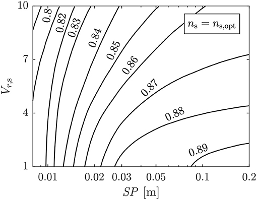
Figure 2. Performance map detailing the effect of the isentropic volume ratio V_r,s and size parameter SP on the maximum isentropic total-to-static efficiency of a radial-inflow turbine (reproduced from Perdichizzi and Lozza, 1987).

One option could be to digitize Figure 2 and calculate V_r,s using a look-up table. However, this approach is not valid since Figure 2 is derived on a kilogram basis, whilst the models described in sections 2.1 and 2.2 are defined on a molar basis. Instead, the authors propose an alternative model. Firstly, from Figure 2 the variation in η_t with V_{r, s} can be evaluated at different size parameters by taking vertical slices through the contour (e.g., for SP = 0.03, η_t = 0.88, 0.87, and 0.86 at V_{r, s} = 2, 4, and 6, respectively etc.). After repeating this process for different size parameters, Figure 3 is obtained. In this figure, each set of results for a particular size parameter are normalized by the maximum efficiency that could be obtained for that size parameter. This is done to remove any variability in η_t due to size effects. Applying a linear regression to this data leads to:

$\begin{array}{ll}\frac{{\eta }_{{\text{V}}_{\text{r}}}}{{\eta }_{\text{max}}}=-0.004615V_{r,\text{s}}+1.007,& (12)\end{array}$

which corresponds to R² = 0.9328. This line is shown by the solid black line in Figure 3.

FIGURE 3

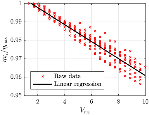
Figure 3. Relationship between the isentropic volume ratio V_r,s and the normalized turbine efficiency. The red crosses correspond to data-points taken from Figure 2 and the black line corresponds to Equation (12).

Using Equation (12) the maximum normalized turbine efficiency (η_Vr/η_max) for a given isentropic volume ratio can be obtained. According to similitude theory, as a turbine design that achieves this efficiency is scaled, the velocities and thermodynamic properties within the turbine, and hence turbine efficiency, will remain the same if the thermodynamic operating conditions and working fluid remain the same. However, in reality, scaling the turbine will lead to a change in turbine efficiency due to changes in the Reynolds number and relative clearance gaps.

The change in efficiency due to a change in the Reynolds number can be estimated from the correlation reported in Baines (2003), which is defined as follows:

$\begin{array}{ll}\frac{1-\eta }{1-{\eta }_{\text{ref}}}=K+(1-K){\left(\frac{R{e}_{\text{ref}}}{Re}\right)}^{0.2},& (13)\end{array}$

where η_ref and Re_ref are the efficiency and Reynolds number of the original turbine, η and Re are the efficiency and Reynolds of the scaled turbine, and K is a constant, which is set to 0.35 (Baines, 2003). The Reynolds number is defined as Re = ṁ/μr, where μ and r are the viscosity and radius at the rotor inlet, respectively. Applying the principle of similitude, the ratio of the Reynolds numbers reduces to a ratio of the blade heights. Hence, after setting the reference efficiency to the value obtained from Equation (12), the change in efficiency due to Reynolds number effects Δη_Re can be estimated as:

$\begin{array}{ll}\Delta {\eta }_{\text{Re}}=(1-{\eta }_{{\text{V}}_{\text{r}}})(1-K)\left({\left(\frac{b_{\text{ref}}}{b}\right)}^{0.2}-1\right),& (14)\end{array}$

where b_ref and b are the rotor inlet blade heights of the original and scaled turbines, respectively.

The enthalpy loss due to clearance losses can be estimated from Dixon (2005):

$\begin{array}{ll}\Delta h_{\text{cl}}=\Delta h_0\left(\frac{\delta }{b_{\text{av}}}\right),& (15)\end{array}$

where Δh₀ is the total enthalpy change across the turbine uncorrected for clearance, δ is the clearance gap, and b_av is the average of the rotor inlet and rotor outlet blade heights. It follows that the change in efficiency due to clearance losses can be calculated from:

$\begin{array}{ll}\frac{\eta }{{\eta }_{\text{ref}}}=\frac{\Delta h_0-\Delta h_{\text{cl}}}{\Delta h_0-\Delta h_{\text{cl},\text{ref}}},& (16)\end{array}$

where η_ref and Δh_{cl, ref} are the efficiency and clearance loss of the original turbine and η and Δh_cl are the efficiency and clearance loss for the scaled turbine. Combining Equations (15, 16), setting η_ref = η_Vr and assuming δ remains constant it follows that:

$\begin{array}{ll}\Delta {\eta }_{\text{cl}}={\eta }_{{\text{V}}_{\text{r}}}\left[\frac{\frac{\delta }{b_{\text{av},\text{ref}}}\left(\frac{b_{\text{av},\text{ref}}}{b_{\text{av}}}-1\right)}{1-\frac{\delta }{b_{\text{av},\text{ref}}}}\right],& (17)\end{array}$

where b_{av, ref} and b_av are the average blade heights for the original and scaled turbine, respectively.

From Equations (14, 17) it is observed that the change in efficiency is dependent on the two blade height ratios. From similitude theory it can be shown that:

$\begin{array}{ll}\frac{b}{b_{\text{ref}}}=\frac{b_{\text{av}}}{b_{\text{av},\text{ref}}}\approx \sqrt{\frac{Ẇ}{{Ẇ}_{\text{ref}}}},& (18)\end{array}$

where Ẇ and Ẇ_ref are the power output from the scaled and original turbines, respectively. This is only approximate since this is derived by assuming the isentropic efficiency of the turbine remains unchanged.

Combining everything, the turbine efficiency for a particular operating condition, defined in terms of V_{r, s}, Δh_ss, and ṁ, can be estimated from:

$\begin{array}{ll}{\eta }_{\text{t}}={\eta }_{{\text{V}}_{\text{r}}}-\Delta {\eta }_{\text{Re}}-\Delta {\eta }_{\text{cl}},& (19)\end{array}$

and the calculation procedure is as follows:

• using an assumed maximum efficiency η_max, calculate η_Vr using Equation (12);

• assuming the turbine efficiency is unchanged when the turbine design is scaled, calculate the turbine power output, Ẇ = ṁη_VrΔh_s;

• using an assumed reference power output Ẇ_ref calculate the blade height ratio (Equation 18);

• calculate the change in efficiency due to Reynolds number and clearance effects (based on an assumed relative clearance gap δ/b_{av, ref}) and hence calculate η_t.

In summary, η_t can be predicted based on three fixed parameters: the maximum efficiency η_max, the relative clearance of the reference turbine δ/b_{av, ref} and a reference power output Ẇ_ref. To identify suitable values for these parameters a parameter optimization study was completed to minimize the average absolute deviation (AAD) between efficiency predictions made using the method developed in this paper, and those reported in Figure 2. For this, a map of operating points was constructed, based on R245fa as the working fluid. To account for variations in V_{r, s}, the expansion process was modeled for p_r ranging between 0.05 and 0.9, with ΔT_sh = 15 K, to a condensation pressure that corresponds T₁ = 303 K. The mass-flow rate was varied between 0.1 and 100 kg/s. Within each step of the optimization process η_t is determined for each operating point for that current set of optimization variables. Moreover, SP is calculated and used to estimate η_t using Figure 2. The AAD between the two maps is calculated, and this is set as the objective function. The efficiency map obtained from this optimization is shown in Figure 4. The values for η_max, δ/b_{av, ref}, and Ẇ_ref are listed in Table 1.

FIGURE 4

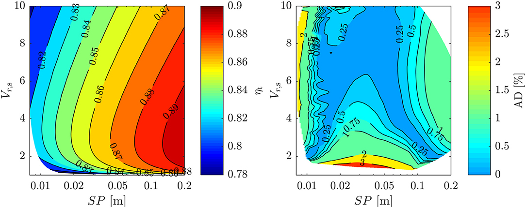
Figure 4. Turbine efficiency map defined by the parameters defined in Table 1 (left), and absolute deviation (AD) between this derived map and the original map in % (right).

TABLE 1

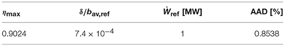
Table 1. Optimal parameter values that minimize the AAD between the turbine model and Figure 2.

It is observed from Figure 4 that for SP > 0.01 and V_{r, s} > 2 the absolute deviation between the model developed in this section and Figure 2 is <2%. At lower volume ratios, a larger deviation is observed, and this is accompanied with the turbine efficiency reducing at low volume ratios which is not observed in the original map. However, similar behavior to that shown in Figure 4 was observed in a more recent study (Lio et al., 2017). Having said this, this deviation is only of minor interest, as it is unlikely than any turbine within an ORC application will have V_{r, s} < 2.

Ultimately, the model enables of η_t to be estimated, based only on thermodynamic properties that can be defined on a kilogram or molar basis. This is extremely useful in thermodynamic optimization studies to consider the effect of the thermodynamic conditions on the turbine performance. However, it should be noted that in deriving this model, data was only available for V_{r, s} ≤ 10, and therefore further studies should be completed to confirm its validity for higher volume ratios.

2.4. Heat-Exchanger Sizing

For the same reasons discussed in section 2.3, of which the most notable is the lack of a simple method to estimate transport properties, a detailed heat-exchanger sizing model has not been included in the ORC system model. Instead, to account for the trade-off between thermodynamic performance and the required heat-transfer areas, a simple heat-exchanger sizing model has been implemented based on assumed values for the overall heat-transfer coefficient in each heat-transfer process.

For a particular heat-transfer process (i.e., preheater, evaporation, superheater, etc.), the required heat-transfer area is found using a discretized heat-exchanger model, which is defined as:

$\begin{array}{ll}A={\displaystyle \sum _{i=1}^n}\frac{ṁ(h_{\text{in},i}-h_{\text{out},i})}{U\Delta T_{\text{log},i}},& (20)\end{array}$

where ṁ is the working-fluid mass-flow rate, h_in and h_out are the enthalpy of the working fluid at the inlet and outlet of the i^th heat-exchanger element, U is the overall heat-transfer coefficient for that particular heat-transfer process and ΔT_log is the counter-flow log-mean temperature difference of the i^th element. The assumed U values for each heat-transfer process are listed in Table 2 and have been selected according to Hewitt (1994). Within this study, the waste-heat source is assumed to be a hot exhaust gas at atmospheric pressure, whilst the heat sink is assumed to be water. Therefore, for other applications, such as a liquid waste-heat stream, or an air-cooled condenser, alternative values to those reported in Table 2 should be used.

TABLE 2

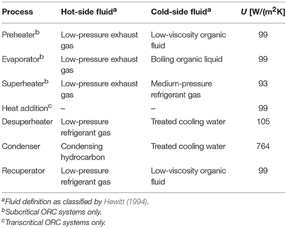
Table 2. Overall heat-transfer coefficients assumed for the different heat-transfer processes. Taken from Hewitt (1994).

The overall heat-transfer coefficient for heat transfer between a hot exhaust gas and a transcritical fluid is not defined by Hewitt (1994). However, it is reasoned that for heat-transfer between a low-pressure exhaust gas and any pressurized fluid, either subcritical or transcritical, the controlling heat-transfer coefficient will be the heat-transfer coefficient on the hot exhaust gas. Therefore, within this study it is assumed that the overall heat-transfer coefficient for transcritical cycles is similar to that of a subcritical cycle.

2.5. Optimization

Within this study two types of optimization will be completed. The first will seek to maximize the net power output, whilst the second will investigate the trade-off between maximizing power output and minimizing the total heat-transfer area. In general, the optimization is formulated as:

$\begin{array}{l}{\displaystyle \underset{\text{x},\text{y}}{min}}\left\{-{Ẇ}_{\text{n}}(\text{x},\text{y}),A(\text{x},\text{y})\right\}\\ \text{subject to:}\\ g(\text{x},\text{y})\le 0\\ h(\text{x},\text{y})\le 0\\ {\text{x}}_{\text{min}}\le \text{x}\le {\text{x}}_{\text{max}}\\ {\text{y}}_{\text{min}}\le \text{y}\le {\text{y}}_{\text{max}}& (21)\end{array}$

where x and y are the vectors defining the working fluid (Equation 3) and ORC system (Equation 9), respectively, g(x, y) and h(x, y) are the fluid and cycle constraints, respectively, and x_min ≤ x ≤ x_max and y_min ≤ y ≤ y_max are the bounds on the optimization variables. The single-objective optimization is completed using the sequential quadratic programming algorithm, suitable for solving non-linear constrained problems, whilst the multi-objective optimization is completed using the multi-objective genetic algorithm optimizer, both available within the Global Optimization Toolbox (MATLAB 2017a, The Mathworks, Inc.).

3. Case Study Definition

For the present study, heat-source temperatures ranging between 100 and 400 °C will be considered, and for each temperature eight different optimizations will be completed. The first four will involve a single-objective optimization aimed at identifying optimal systems that maximize Ẇ_n. These will consider both subcritical and transcritical cycles, and will be completed using either a fixed efficiency turbine model or the variable efficiency turbine model proposed in section 2.3. The second set of four optimizations will follow the same format, but will consider a multi-objective optimization. Overall, this will allow a complete investigation into the effects of the cycle architecture, turbine performance and the optimization objective on the optimal system parameters.

The case study follows that defined in White and Sayma (2018). The assumptions for this study are listed in Table 3. The heat source is hot exhaust gas at atmospheric pressure and the heat sink is water at T_ci = 288 K; hence the specific-heat capacities are set to c_{p, h} = 1 kJ/(kgK) and c_{p, c} = 4.2 kJ/(kgK), respectively. Moreover, the heat-sink and heat-source mass-flow rates are assumed to be equal, and hence τ = (ṁ_cp)c/(ṁ_cp)h = 4.2. However, it is noted that in the same previous paper it was shown that increasing this to τ = 100 did not significantly affect the optimal working fluid, with the maximum deviation between the optimal critical temperature for the τ = 100 and τ = 4.2 cases being <4%. Finally, to remove any scale effects on the turbine performance, ṁ_h for each value of T_hi is scaled so the power output from the system is ≈25 kW for all cases. To do this, the first optimization, which identifies the optimal subcritical cycle that maximizes Ẇ_n and is based on a constant efficiency turbine model, is completed for all heat-source temperatures assuming ṁ_h = 1 kg/s. The power output from this optimization is then used to obtain the scaled mass-flow rate (i.e., ṁ_h = 25/Ẇ_n) that is used in subsequent optimizations.

TABLE 3

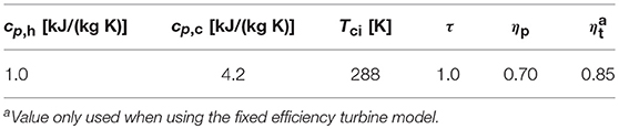
Table 3. Fixed parameters for the optimization case study.

The optimization variables and constraints are similar to those defined in the authors' previous paper, and are briefly summarized in Table 4. The main thing to note is that p_cr and ω are not included as variables, but are fixed to p_cr = 30 bar and ω = 0.3, respectively. As shown in Figure 5, this is found to accurately capture the relationship between critical temperature and normal boiling temperature that is observed for a range of common working fluids. These fluids include common hydrocarbons (n-alkanes, methyl-alkanes, cyclo-alkanes and aromatics with 21 ≤ p_cr ≤ 56 bar and 0.13 ≤ ω ≤ 0.39), siloxanes (9 ≤ p_cr ≤ 14 bar; 0.53 ≤ ω ≤ 0.83), and refrigerants (hydrofluorocarbons and hydrofluoroolefins with 29 ≤ p_cr ≤ 42 bar and 0.27 ≤ ω ≤ 0.38), alongside ammonia, ethanol, methanol, and Novec 649 and Novec 774. Moreover, a sensitivity study showed that ω has little effect on the optimal critical temperature for a particular heat source, whilst the percentage difference in power output for different values of ω varied by <2% (White and Sayma, 2018).

TABLE 4

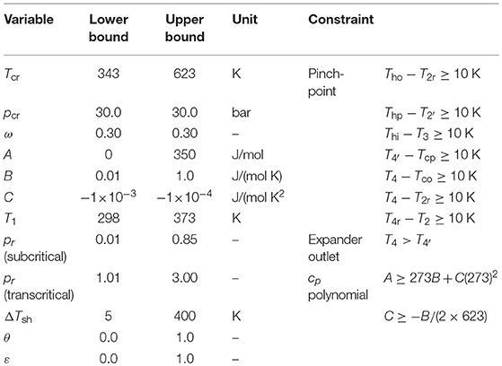
Table 4. Variables and constraints for the optimization case study.

FIGURE 5

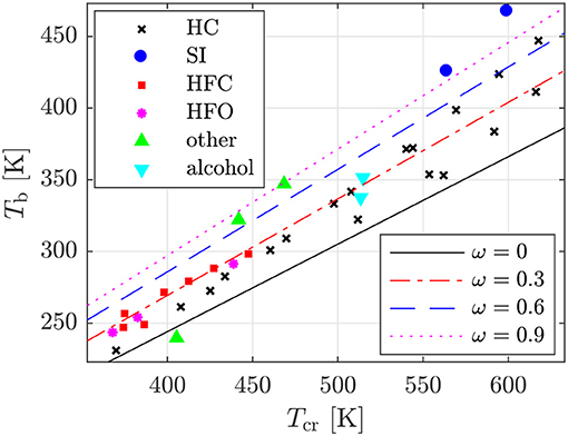
Figure 5. Critical temperature T_cr and normal-boiling temperature T_b of common working fluids available within the REFPROP program (markers) and the same parameters obtained using the Peng-Robinson equation of state for different values of ω with p_cr = 30 bar (lines). HC, hydrocarbons; SI, siloxanes; HFC, hydrofluorocarbons; HFO, hydrofluoroolefins.

4. Results and Discussion

4.1. Results From the Power Output Optimization

The first results to evaluate are the optimal systems that maximize the power output from each source (Figure 6). Before discussing these results, it is worth noting that, in all cases, the optimization converged to a solution with no recuperator (i.e., ε = 0), thus reaffirming the conclusion found within the literature that for unconstrained waste-heat streams there is little benefit in recuperation.

FIGURE 6

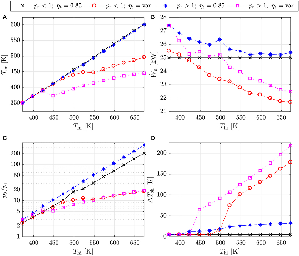
Figure 6. Optimal subcritical (p_r < 1) and transcritical (p_r > 1) cycles for different heat-source temperatures obtained using a fixed turbine efficiency (η_t = 0.85) and the variable efficiency model (η_t = var.): (A) Optimal critical temperatures; (B) net power output; (C) cycle pressure ratio; and (D) amount of superheat.

4.1.1. Working Fluid and Cycle Parameters

Previously, the authors have shown that, for a subcritical, non-recuperated ORC system, the optimal fluid critical temperature can be found using a linear correlation (T_cr = 0.830T_hi + 41.27) (White and Sayma, 2018). Referring to Figure 6A, the results for the subcritical, fixed expander efficiency optimization agree with this previous result. This is not surprising as the setup for both studies is the same, however, in the present study it is also observed that the transcritical, fixed expander efficiency optimizations identify optimal systems with very similar critical temperatures. This suggests that from a thermodynamic point of view the optimal fluid is independent of the cycle architecture.

As observed in Figure 6C, the increase in T_cr with T_hi in both the fixed efficiency subcritical and transcritical optimizations is associated with an increase in the cycle pressure ratio, which follows a power law. Therefore, for high-temperature heat sources the optimal pressure ratio is very high; more specifically, for T_hi > 600 K, the optimal pressure ratio exceeds 50. Pressure ratios this high are likely to have a significant effect on expander performance, particularly if it is a single-stage machine, and will also result in a sub-atmospheric condensation pressure, leading to not only physically large condensers, but also design challenges surrounding the prevention of air ingress.

In comparison, the results obtained using the variable efficiency model are significantly different. Firstly, the optimal value of T_cr still increases with T_hi, but the increase is no longer linear. For T_hi < 423 K, the optimal values for T_cr for the optimizations with the fixed and variable efficiency expander models are similar. However, above this temperature, to avoid significantly large volumetric expansion ratios, which lead to a reduction in the turbine efficiency, the increasing heat-source temperature is utilized by superheating the working fluid (Figure 6D), rather than increasing T_cr and maintaining a relatively low superheat. Consequently, the pressure ratios are reduced by an order of magnitude. In other words, the optimal thermodynamic cycles, identified using the fixed efficiency model, represent operating conditions where turbine performance is poor. Therefore, when the turbine is considered, thermodynamic performance is sacrificed in favor of improving turbine performance. Moreover, this reduction in cycle pressure also has the advantage of removing sub-atmospheric operating conditions.

It is also useful to highlight a number of findings not been reported in Figure 6 for brevity. Firstly, for all cycles, the optimal condensation temperature is similar, and increases linearly with T_hi. This behavior is observed since an increase in T_hi implies an increase in the heat available, and therefore an increase in the amount of heat that must be rejected to the heat sink. This, in turn, requires a larger heat-sink temperature increase, which increases the condensation temperature. Secondly, it is noted that whilst the working-fluid mass-flow rate reduces as T_hi increases, the difference in the mass-flow rate between the different cycles does not change significantly. With regards to the shape of the saturation dome for the optimal cycles, as defined by the optimized values of A, B, and C, it is found that when a fixed expander efficiency is assumed, the optimal fluid always has a saturated vapor line with a positive gradient. This result is found for both the subcritical and transcritical cycles. However, when the variable efficiency expander model is used, and the optimization converges on a cycle with a high superheat (i.e., the high-temperature systems), there appears to be a transition to fluids with a saturated vapor line that has a positive gradient. The reason for this is not yet fully apparent, but will be investigated in future studies.

Finally, for all the subcritical optimizations, the optimization converges on a system with the maximum reduced pressure (p_r = 0.85). This minimizes the latent-heat of vaporization, which in turn, minimizes the amount of isothermal heat exchange in the evaporator, and hence reduces exergy destruction. With regards to the variation in p_r for the transcritical cycles, these are reported in Figure 7. Combining these results with those reported in Figure 6A it is observed that the thermodynamically optimal transcritical cycles (η_t = 0.85) require fluids with high critical temperatures, but the maximum reduced pressure within the cycle remains <1.5. On the other hand, the optimal transcritical cycles identified using the variable efficiency turbine model require much lower critical temperatures, but to compensate require higher reduced pressures. This could suggest that in practical transcritical systems, the required evaporation pressure could be very high, which could have both technical and economic implications on the design of the system.

FIGURE 7

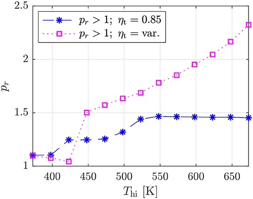
Figure 7. Evaporator reduced pressure for the optimal transcritical systems obtained using the fixed efficiency and variable efficiency turbine model.

4.1.2. Turbine Efficiency and Power Output

The turbine efficiencies, and variation in SP and V_{r, s}, for the optimal subcritical and transcritical systems obtained using the variable efficiency model are shown in Figure 8. The results shown in Figure 8B start on the right-hand side, and move from right to left as T_hi increases, and are reported on a molar basis, and hence cannot be directly compared with Figure 4.

FIGURE 8

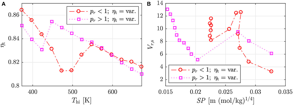
Figure 8. Turbine performance for the optimal subcritical (p_r < 1) and transcritical (p_r > 1) cycles for different heat-source temperatures obtained using the variable efficiency model: (A) turbine efficiency; and (b) expansion parameters.

For the subcritical cycles, the lowest temperature system starts with a high turbine efficiency, owing to low and relatively high values for V_{r, s} and SP, respectively. As T_hi increases, SP begins to reduce, whilst V_{r, s} increases rapidly, which, in turn, leads to a drop in efficiency. However, until this point, the cycle operating conditions are the same as the thermodynamic optimal conditions identified using the fixed efficiency model. After this, a transitional period is observed where SP and V_{r, s} simultaneously reduce and η_t increases, and this represents the point where the cycle operating conditions begin to deviate from the thermodynamic optimum, in search of higher turbine efficiencies. However, this can only occur for a short while until the drop in thermodynamic performance becomes significant enough that it is better to again sacrifice turbine performance. At this point, the optimal systems settle around a size parameter of ≈0.0225, and increasing T_hi is accommodated by increasing ΔT_sh. This, in turn, causes a gradual increase in the V_{r, s} and a reduction in η_t. For the transcritical cycles, similar behavior is observed as T_hi increases, although a transitional period is not observed, with a sudden jump in η_t observed instead.

Referring back to Figure 6, the net power outputs obtained from the four different optimizations are summarized in Figure 6B. Comparing the results obtained for a fixed turbine efficiency, it is observed that the transcritical cycles produce more power than the subcritical cycles for all heat-source temperatures, although the difference reduces as T_hi increases. More specifically, at T_hi = 373 K, the optimal transcritical cycle produces 9.7% more power than the optimal subcritical cycle, whilst this reduces to only 0.9% for T_hi = 648 K. This reduction can be associated with a reduction in the evaporator load, relative to the total load for the heat addition process [i.e., $(h_{3^{\prime }}-h_{2^{\prime }})/(h_3-h_{2\text{r}})$], for the subcritical cycles as T_hi increases. In other words, as T_hi increases, a larger proportion of the heat-transfer into the subcritical ORC occurs in the preheater, rather than in the evaporator. As the two-phase heat transfer in the evaporator is isothermal, it is associated with a large amount of exergy destruction. Therefore, reducing the evaporator load reduces this exergy destruction, and leads to better thermodynamic performance.

It is also observed from Figure 6B that using the variable turbine efficiency model, and the subsequent change in the thermodynamic operating conditions, has a significant effect on the net power output for both the subcritical and transcritical cycles. In general, the variable turbine efficiency model results in a reduction in the power output that can be produced, and the relative reduction in power increases as T_hi increases. For the subcritical systems, the relative change in net power output ranges between +2.0 and −13.2% for heat-source temperatures of 373 and 673 K, respectively. For the transcritical systems, the relative change ranges between 0.0 and −11.5%. This reduction in power output when using the variable efficiency model can be partly attributed to a reduction in the turbine efficiency (Figure 8), but also the result of the reduction in the cycle pressure ratio, as discussed previously. Ultimately, these results show that both the power output, and the cycle operating conditions, are quite different when the variable efficiency model is used instead of assuming a fixed isentropic efficiency. This demonstrates the importance of accounting for expander performance during working-fluid selection and cycle optimization studies. Comparing the results obtained for subcritical and transcritical cycles with the variable turbine efficiency model, it is observed that the optimal transcritical cycles generate more power than the subcritical cycles (Figure 6B). In particular, the increase in power output for the transcritical systems ranges between +2.1 and +7.8% for heat-source temperatures of 423 and 498 K, respectively.

4.1.3. Component Design Aspects

Overall, from the point of view of maximizing Ẇ_n, transcritical systems achieve better performance than subcritical systems (Figure 6). However, transcritical cycle have implications on the design of the system, owing to higher operating pressures. Moreover, maximizing Ẇ_n leads to systems associated with higher costs, due to large heat-transfer areas. Therefore, as a preliminary evaluation, the total required heat-transfer area for the different optimal systems are shown in Figure 9.

FIGURE 9

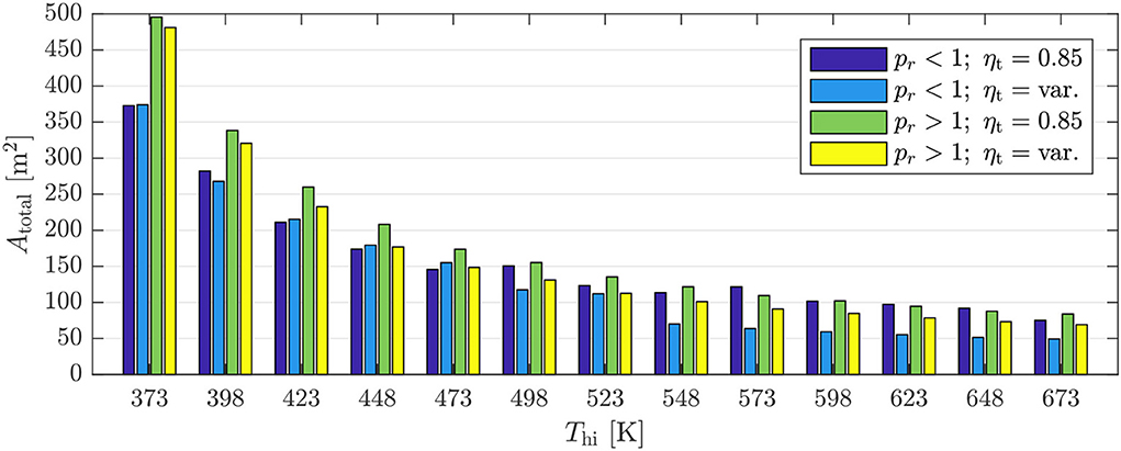
Figure 9. Total heat-transfer area required for the optimal subcritical (p_r < 1) and transcritical (p_r > 1) cycles for different heat-source temperatures obtained using a fixed turbine efficiency (η_t = 0.85) and the variable efficiency model (η_t = var.).

Firstly, despite the power output being similar in all cases, the low-temperature systems require significantly more heat-transfer area than the higher-temperature systems. It follows that the low-temperature systems will be associated with higher investment costs, as well-described within the literature. Comparing the results for the subcritical and transcritical results obtained with the fixed efficiency model, it is found that for T_hi ≤ 473 K, the transcritical cycles produce between 9.7 and 3.9% extra power, but require between 32.9 and 19.2% more heat-transfer area, respectively. Above 473 K the difference is less significant, owing to the reduced two-phase heat transfer in the optimal subcritical systems.

The results for the subcritical systems suggest that the subcritical cycles identified when considering turbine performance within the optimization actually result in significantly lower heat-transfer areas than the thermodynamically optimal systems, particularly for higher heat-source temperatures. More specifically, for T_hi ≥ 548 K, the subcritical systems are associated with a reduction in heat-transfer area between 34.5 and 43.9%, compared to the thermodynamically optimal cycles, with a reduction in power between 8.9 and 13.2%. Moreover, these systems are associated with a reduction in heat-transfer area between 28.9 and 30.6%, compared to the transcritical cycles identified using the variable efficiency model, with power reductions between 3.5 and 4.9%. These significant reductions are associated with the large amount of superheating that is required for the subcritical cycles, which leads to a relatively large proportion of the heat-addition process into the ORC occurring across a large temperature difference (relative to the temperature difference in the preheater). Moreover, the increasing superheat at the expander inlet is also associated with a larger superheat at the expander outlet, which also leads to both a larger desuperheater load, and a larger temperature difference within the desuperheater. These combined effects are a source of increasing irreversibility within the cycle, leading to a reduction in power output, but evidently a significant reduction in the required heat-transfer area.

4.2. Results From the Multi-Objective Optimization

To investigate in more detail the trade-off between thermodynamic performance, and the size of the heat exchangers, a multi-objective optimization for each case has been conducted. The Pareto fronts obtained from these optimizations for subcritical and transcritical cycles, both with the fixed and variable efficiency turbine models, are shown for the 373, 473, 573, and 673 K heat-source temperatures in Figure 10.

FIGURE 10

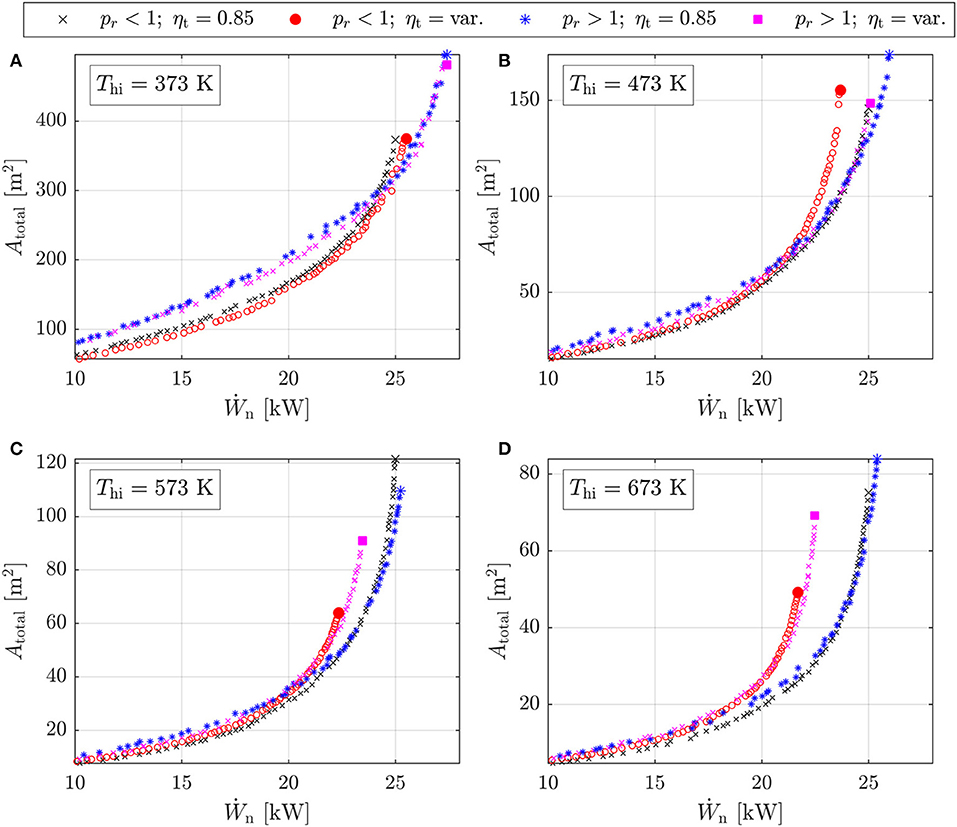
Figure 10. Pareto fronts identified from the multi-objective optimization for the subcritical (p_r < 1) and transcritical (p_r > 1) cycles using the fixed (η = 0.85) and variable (η = var.) efficiency models: (A) T_hi = 373 K; (B) T_hi = 473 K; (C) T_hi = 573 K; (D) T_hi = 673 K.

For the 373 K heat source (Figure 10A), there is no significant difference between the Pareto fronts for the fixed and variable turbine efficiency models. In other words, for low heat-source temperatures, the pressure ratios within the optimal thermodynamic cycles are sufficiently low such that turbine efficiency is not compromised; this reaffirms the observations in Figure 6. Secondly, for power outputs below 24 kW, subcritical cycles are capable of generating the same power output as a transcritical cycle, but with smaller heat exchangers, whilst for larger power outputs transcritical outperform subcritical cycles. Therefore, if one is interested in maximizing the power output from this heat source, a transcritical cycle should be selected, but from a more economic perspective, a subcritical cycle would be more suitable.

For the 473 K heat source (Figure 10B), a larger difference between the Pareto fronts obtained using the fixed and variable turbine efficiency models is observed, particularly for the subcritical cycles. These results are in-line with those reported in Figure 6, and are observed because at this temperature the optimal thermodynamic cycles begin to require larger pressure ratios which are detrimental to turbine efficiency. When comparing subcritical and transcritical cycles, it is observed that for power outputs below 20 kW, subcritical cycles perform the best, generating the same power output but with smaller heat exchangers. However, to obtain maximum heat recovery, transcritical cycles are more suitable.

Finally, for both the 573 and 673 K heat sources similar observations are made. The power output for both cycles, obtained using the variable turbine efficiency model, are lower than the power outputs obtained when using the fixed efficiency model. This demonstrates the importance of considering the turbine performance within the cycle optimization, particularly at higher heat-source temperatures. Comparing subcritical and transcritical cycles, it is again observed that transcritical cycles are the optimal choice in terms of maximizing power output. However, up until the maximum power point for the subcritical system, the thermodynamic performance and corresponding heat-transfer area requirements are similar for both the subcritical and transcritical systems. In other words, either cycle is a suitable. However, considering that transcritical cycles are associated with higher operating pressures, which, in turn, are associated with higher costs, it is likely that subcritical cycles may offer the most economical choice.

Besides comparing the Pareto fronts, it is also worth considering the fluid and cycle parameters for the cycles that form the Pareto fronts. For brevity, these results are not reported in detail, and instead will be briefly summarized. Firstly, the optimal condensation temperature T₁, reduced evaporation pressures p_r, and amount of superheat ΔT_sh are not found to vary significantly across each Pareto front. That is not to say that they do not vary between the different cycle architectures and heat-source temperatures, but that for a particular heat source and cycle architecture the optimal values for these parameters are not significantly affected by whether the objective is to maximize power output, or minimize heat-transfer area.

The optimal values for T_cr for each Pareto front are reported in Figure 11. In this plot, the results for each type of optimization (i.e., subcritical and transcritical either with the fixed or variable turbine efficiency model) are reported in the form of a box plot. Alongside this, the dashed-black boxes correspond to ±3% of the mean critical temperature for the Pareto front. These results show that, besides a few outliers for the transcritical cycles for the 473 and 673 K heat-source temperatures, all of the critical temperatures that lie on the Pareto front are within ±3% of the mean critical temperature. In other words, across the Pareto front there is no significant change in the optimal value for T_cr, and therefore the optimum is independent of whether the objective is to maximize power output or minimize heat-transfer area. On the other hand, the optimal critical temperature appears to be more dependent on the cycle architecture, and also on the performance of the expander.

FIGURE 11

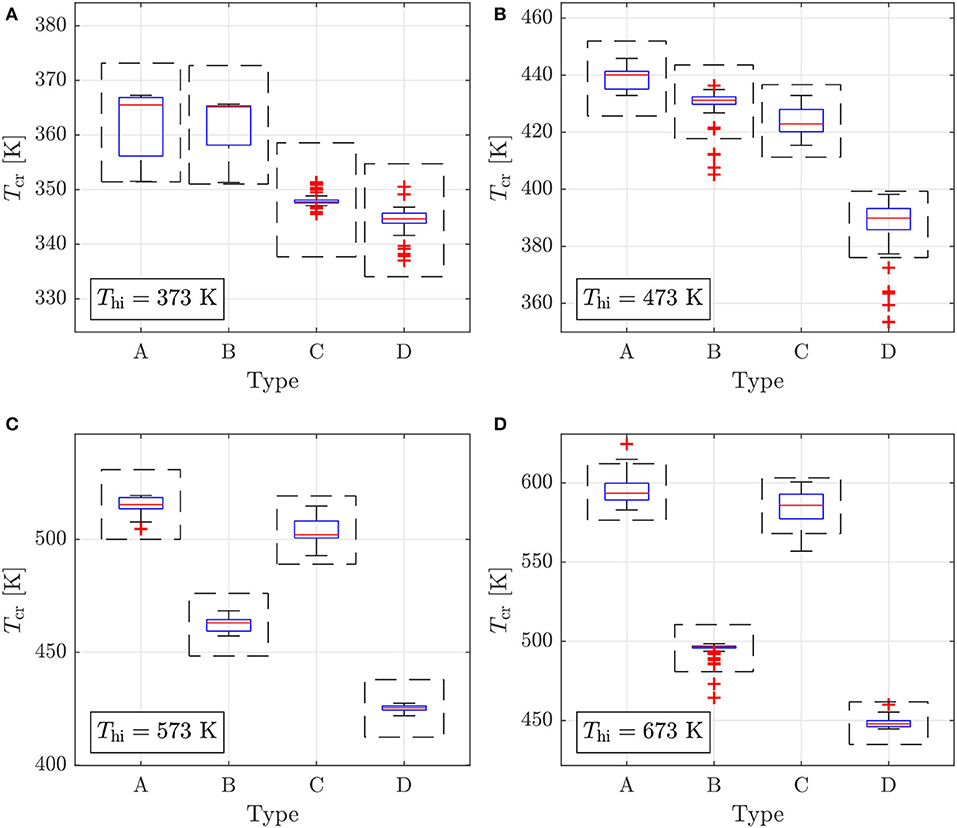
Figure 11. Box plots for the optimal critical temperatures T_cr that lie on the Pareto front for each optimization type (A: subcritical, η = 0.85; B: transcritical, η = 0.85; C: subcritical η = var.; D: transcritical η = var.). The black-dashed lines correspond to ±3% of the mean critical temperature, whilst the red crosses represent the outliers of the dataset.

From the observations for T_cr, T₁, p_r, and ΔT_sh it is inferred that the pressure ratio does not significantly change across the Pareto front, and neither do the state points in each cycle. Instead, the main parameter that controls the trade-off between thermodynamic performance and total heat-transfer area is the non-dimensional heat-source temperature drop θ, and for which a near-linear correlation between θ and Ẇ_n is observed across the Pareto front. This suggests that the optimal working fluid (i.e., critical temperature) and cycle operating conditions can be identified based on a single-objective optimization based on power output, and then modified to meet the power output and heat-transfer area requirements by adjusting θ. In other words, the optimal working fluid for a particular heat-source temperature can be identified from the results reported in Figure 6A. Neglecting expander performance, the optimal working-fluid critical temperature for either a subcritical or transcritical cycle can be identified through a linear correlation, such as that reported previously (White and Sayma, 2018). For a more realistic estimate, accounting for expander performance, a simple linear correlation cannot be derived, but none the less a qualitative assessment of Figure 6A can be used to identify the optimal working fluid. Finally, it is worth noting that within our previous study (White and Sayma, 2018), the results from the optimization, in which theoretically optimal working fluids were identified, were compared to results from an optimization completed for physical working fluids using REFPROP. The results showed that for heat-source temperatures below 120 °C the maximum deviation between the two models was 18%, but this reduced to 5% for heat-source temperatures exceeding 220 °C. This gives good confidence in the ability of the model to identify solutions that represent realistic ORC systems operating with physical working fluids.

5. Conclusions

Within this paper an integrated optimization framework for ORC systems has been proposed that can optimize fluid parameters and cycle conditions for different cycle architectures, whilst accounting for the effects of these parameters on the turbine performance. The latter has been achieved by developing a novel model to estimate the design-point turbine efficiency based only on the thermodynamic operating conditions.

The results indicate that including expander performance within the optimization process results in significantly different cycles to thermodynamically optimal cycles obtained by assuming a fixed turbine efficiency. More specifically, the pressure ratios in the former are reduced by an order of magnitude. Moreover, as heat-source temperature increases, the power outputs predicted using the variable efficiency model reduce, and reach a maximum reduction of 13.2 and 11.5% compared to the optimal cycles for subcritical and transcritical cycles, respectively. Comparing subcritical and transcritical cycles that generate maximum power from the defined waste-heat streams, transcritical cycles could produce between 2.1 and 7.8% more power than their subcritical counterparts. However, results from the multi-objective optimization studies suggest that when the trade-off between power output and heat-transfer area is considered, and power output is slightly reduced in favor of smaller heat exchangers, subcritical cycles can produce the same power output as transcritical cycles, but require smaller heat exchangers. This suggests that from an economic point of view subcritical cycles are more optimal. Finally, it is found that the optimal working-fluid critical temperature does not vary significantly across the Pareto front, but depends on the cycle architecture and the heat-source temperature. Consequently, within cycle optimization studies it may be suitable to conduct fluid selection based on a thermodynamic optimization, and subsequently adjust the heat-source temperature drop to meet the required trade-off between performance and heat exchanger size.

The next steps in this work are to validate further the expander model developed in this study, and implement a more detailed heat-exchanger sizing methodology. Moreover, there is the need to investigate the applicability of these results to a wider group of heat sources and heat sinks, including heat sinks with a smaller or larger heat capacity, and to consider liquid waste-heat streams or air-cooled systems.

Author Contributions

MW conceived and developed the methodology, conducted the case study, analyzed the data, and wrote the paper. AS provided valuable advice and feedback throughout the development of this research and preparation of the paper, and was responsible for proofreading the paper before submission.

Funding

This work was supported by the UK Engineering and Physical Sciences Research Council (EPSRC) [grant number: EP/P009131/1].

Conflict of Interest Statement

The authors declare that the research was conducted in the absence of any commercial or financial relationships that could be construed as a potential conflict of interest.

References

Andreasen, J., Kærn, M., Pierobon, L., Larsen, U., and Haglind, F. (2016). Multi-objective optimization of organic Rankine cycle power plants using pure and mixed working fluids. Energies 9:322. doi: 10.3390/en9050322

CrossRef Full Text | Google Scholar

Angelino, G., and Colonna, P. (1998). Multicomponent working fluids for organic Rankine cycles (ORCs). Energy 23, 449–463. doi: 10.1016/S0360-5442(98)00009-7

CrossRef Full Text | Google Scholar

Astolfi, M., and Macchi, E. (2015). “Efficiency correlations for axial flow turbines working with non-conventional fluids,” in 3rd International Seminar on ORC Power Systems (Brussels), 12–14 October, 83.

Google Scholar

Bahamonde, S., Pini, M., De Servi, C., Rubino, A., and Colonna, P. (2017). Method for the preliminary fluid dynamic design of high-temperature mini-organic Rankine cycle turbines. J. Eng. Gas Turbines Power 139:082606. doi: 10.1115/1.4035841

CrossRef Full Text | Google Scholar

Baines, N. (2003). “Chapter 7–9: Radial turbine design, Part 3,” in Axial and Radial Turbines, eds H. Moustapha, M. F. Zelesky, N. C. Baines, and D. Japikse (Concepts ETI), 198–326.

Brignoli, R., and Brown, J. S. (2015). Organic Rankine cycle model for well-described and not-so-well-described working fluids. Energy 86, 93–104. doi: 10.1016/j.energy.2015.03.119

CrossRef Full Text | Google Scholar

Chapman, W. G., Gubbins, K. E., Jackson, G., and Radosz, M. (1990). New reference equation of state for associating liquids. Ind. Eng. Chem. Res. 29, 1709–1721. doi: 10.1021/ie00104a021

CrossRef Full Text | Google Scholar

Chen, H., Goswami, D. Y., and Stefanakos, E. K. (2010). A review of thermodynamic cycles and working fluids for the conversion of low-grade heat. Renew. Sustain. Energy Rev. 14, 3059–3067. doi: 10.1016/j.rser.2010.07.006

CrossRef Full Text | Google Scholar

Cignitti, S., Andreasen, J. G., Haglind, F., Woodley, J. M., and Abildskov, J. (2017). Integrated working fluid-thermodynamic cycle design of organic Rankine cycle power systems for waste heat recovery. Appl. Energy 203, 442–453. doi: 10.1016/j.apenergy.2017.06.031

CrossRef Full Text | Google Scholar

Dixon, S. L. (2005). Fluid Mechanics and Thermodynamics of Turbomachinery. 5th Edn. Oxford: Butterworth-Heinemann.

Google Scholar

Fischer, J. (2011). Comparison of trilateral cycles and organic Rankine cycles. Energy 36, 6208–6219. doi: 10.1016/j.energy.2011.07.041

CrossRef Full Text | Google Scholar

Hewitt, G. (1994). Selection and Costing of Heat Exchangers. Technical report, ESDU 92013.

Imran, M., Haglind, F., Asim, M., and Zeb Alvi, J. (2018). Recent research trends in organic Rankine cycle technology: a bibliometric approach. Renew. Sustain. Energy Rev. 81, 552–562. doi: 10.1016/j.rser.2017.08.028

CrossRef Full Text | Google Scholar

Lampe, M., Stavrou, M., Bu, H. M., Gross, J., and Bardow, A. (2014). Simultaneous optimization of working fluid and process for organic Rankine cycles using PC-SAFT. Ind. Eng. Chem. Res. 53, 8821–8830. doi: 10.1021/ie5006542

CrossRef Full Text | Google Scholar

Lampe, M., Stavrou, M., Schilling, J., Sauer, E., Gross, J., and Bardow, A. (2015). Computer-aided molecular design in the continuous-molecular targeting framework using group-contribution PC-SAFT. Comput. Chem. Eng. 81, 278–287. doi: 10.1016/j.compchemeng.2015.04.008

CrossRef Full Text | Google Scholar

Lecompte, S., Huisseune, H., van den Broek, M., De Schampheleire, S., and De Paepe, M. (2013). Part load based thermo-economic optimization of the Organic Rankine Cycle (ORC) applied to a combined heat and power (CHP) system. Appl. Energy 111, 871–881. doi: 10.1016/j.apenergy.2013.06.043

CrossRef Full Text | Google Scholar

Lemmon, E., Huber, M., and McLinden, M. (2013). NIST Standard Reference Database 23: Reference Fluid Thermodynamic and Transport Properties-REFPROP. Gaithersburg, MD: National Institute for Standards and Technology (NIST).

Google Scholar

Lio, L. D., Manente, G., and Lazzaretto, A. (2017). A mean-line model to predict the design efficiency of radial inflow turbines in organic Rankine cycle (ORC) systems. Appl. Energy 205, 187–209. doi: 10.1016/j.apenergy.2017.07.120

CrossRef Full Text | Google Scholar

Macchi, E., and Perdichizzi, A. (1981). Efficiency prediction for axial-flow turbines operating with nonconventional fluids. J. Eng. Power 103, 718–724. doi: 10.1115/1.3230794

CrossRef Full Text | Google Scholar

Meroni, A., Andreasen, J. G., Persico, G., and Haglind, F. (2018). Optimization of organic Rankine cycle power systems considering multistage axial turbine design. Appl. Energy 209, 339–354. doi: 10.1016/j.apenergy.2017.09.068

CrossRef Full Text | Google Scholar

Mounier, V., Olmedo, L. E., and Schiffmann, J. (2018). Small scale radial inflow turbine performance and pre-design maps for Organic Rankine Cycles. Energy 143, 1072–1084. doi: 10.1016/j.energy.2017.11.002

CrossRef Full Text | Google Scholar

Oyewunmi, O., and Markides, C. (2016). Thermo-economic and heat transfer optimization of working-fluid mixtures in a low-temperature organic Rankine cycle system. Energies 9:448. doi: 10.3390/en9060448

CrossRef Full Text | Google Scholar

Oyewunmi, O. A., Taleb, A. I., Haslam, A. J., and Markides, C. N. (2016). On the use of SAFT-VR Mie for assessing large-glide fluorocarbon working-fluid mixtures in organic Rankine cycles. Appl. Energy 163, 263–282. doi: 10.1016/j.apenergy.2015.10.040

CrossRef Full Text | Google Scholar

Palma-Flores, O., Flores-Tlacuahuac, A., and Canseco-Melchor, G. (2016). Simultaneous molecular and process design for waste heat recovery. Energy 99, 32–47. doi: 10.1016/j.energy.2016.01.024

CrossRef Full Text | Google Scholar

Papadopoulos, A. I., Stijepovic, M., and Linke, P. (2010). On the systematic design and selection of optimal working fluids for organic Rankine cycles. Appl. Thermal Eng. 30, 760–769. doi: 10.1016/j.applthermaleng.2009.12.006

CrossRef Full Text | Google Scholar

Papadopoulos, A. I., Stijepovic, M., Linke, P., Seferlis, P., and Voutetakis, S. (2013). Toward optimum working fluid mixtures for organic Rankine cycles using molecular design and sensitivity analysis. Ind. Eng. Chem. Res. 52, 12116–12133. doi: 10.1021/ie400968j

CrossRef Full Text | Google Scholar

Peng, D.-Y., and Robinson, D. B. (1976). A new two-constant equation of state. Ind. Eng. Chem. Fundam. 15, 59–64. doi: 10.1021/i160057a011

CrossRef Full Text | Google Scholar

Perdichizzi, A., and Lozza, G. (1987). “Design criteria and efficiency prediction for radial inflow turbines,” in Gas Turbine Conference and Exhibition (Anaheim, CA), May 31–June 4, 87–GT–231.

Google Scholar

Pierobon, L., Nguyen, T. V., Larsen, U., Haglind, F., and Elmegaard, B. (2013). Multi-objective optimization of organic Rankine cycles for waste heat recovery: application in an offshore platform. Energy 58, 538–549. doi: 10.1016/j.energy.2013.05.039

CrossRef Full Text | Google Scholar

Quoilin, S., Declaye, S., Tchanche, B. F., and Lemort, V. (2011). Thermo-economic optimization of waste heat recovery organic Rankine cycles. Appl. Thermal Eng. 31, 2885–2893. doi: 10.1016/j.applthermaleng.2011.05.014

CrossRef Full Text | Google Scholar

Saleh, B., Koglbauer, G., Wendland, M., and Fischer, J. (2007). Working fluids for low-temperature organic Rankine cycles. Energy 32, 1210–1221. doi: 10.1016/j.energy.2006.07.001

CrossRef Full Text | Google Scholar

Schilling, J., Lampe, M., and Bardow, A. (2016). 1-stage CoMT-CAMD: an approach for integrated design of ORC process and working fluid using PC-SAFT. Chem. Eng. Sci. 159, 217–230. doi: 10.1016/j.ces.2016.04.048

CrossRef Full Text | Google Scholar

Schilling, J., Tillmanns, D., Lampe, M., Hopp, M., Gross, J., and Bardow, A. (2017). From molecules to dollars: integrating molecular design into thermo-economic process design using consistent thermodynamic modeling. Mol. Syst. Des. Eng. 2, 301–320. doi: 10.1039/C7ME00026J

CrossRef Full Text | Google Scholar

Schwoebel, J. A. H., Preissinger, M., Brueggemann, D., and Klamt, A. (2017). High-throughput screening of working fluids for the organic Rankine cycle (ORC) based on conductor-like screening model for realistic solvation (COSMO-RS) and thermodynamic process simulations. Ind. Eng. Chem. Res. 56, 788–798. doi: 10.1021/acs.iecr.6b03857

CrossRef Full Text | Google Scholar

Soave, G. (1972). Equilibrium constants from a modified Redlich-Kwong equation of state. Chem. Eng. Sci. 27, 1107–1203. doi: 10.1016/0009-2509(72)80096-4

CrossRef Full Text | Google Scholar

Su, W., Zhao, L., and Deng, S. (2017a). Developing a performance evaluation model of organic Rankine cycle for working fluids based on the group contribution method. Energy Conv. Manage. 132, 307–315. doi: 10.1016/j.enconman.2016.11.040

CrossRef Full Text | Google Scholar

Su, W., Zhao, L., and Deng, S. (2017b). Simultaneous working fluids design and cycle optimization for Organic Rankine cycle using group contribution model. Appl. Energy 202, 618–627. doi: 10.1016/j.apenergy.2017.03.133

CrossRef Full Text | Google Scholar

Tartière, T., and Astolfi, M. (2017). A world overview of the organic Rankine cycle Market. Energy Proc. 129, 2–9. doi: 10.1016/j.egypro.2017.09.159

CrossRef Full Text

van Kleef, L. M. T., Oyewunmi, O. A., Harraz, A. A., Haslam, A. J., and Markides, C. N. (2018). “Case studies in computer-aided molecular design (CAMD) of low- and medium-grade waste-heat recovery ORC systems,” in The 31st International Conference on Efficiency, Cost, Optimization, Simulation and Environmental Impact of Energy Systems (Guimarães), 17th–22nd June.

Google Scholar

White, M., and Sayma, A. (2018). A generalised assessment of working fluids and radial turbines for non-recuperated subcritical organic rankine cycles. Energies, 11(4):800. doi: 10.3390/en11040800

CrossRef Full Text | Google Scholar

White, M. T., Oyewunmi, O. A., Chatzopoulou, M. A., Pantaleo, A. M., Haslam, A. J., and Markides, C. N. (2018). Computer-aided working-fluid design, thermodynamic optimisation and thermoeconomic assessment of ORC systems for waste-heat recovery. Energy 161, 1181–1198. doi: 10.1016/j.energy.2018.07.098

CrossRef Full Text | Google Scholar

White, M. T., Oyewunmi, O. A., Haslam, A. J., and Markides, C. N. (2017). Industrial waste-heat recovery through integrated computer-aided working-fluid and ORC system optimisation using SAFT-Γ Mie. Energy Conv. Manage. 150, 851–869. doi: 10.1016/j.enconman.2017.03.048

CrossRef Full Text | Google Scholar