Typical Periods for Two-Stage Synthesis by Time-Series Aggregation with Bounded Error in Objective Function

Two-stage synthesis problems simultaneously consider here-and-now decisions (e.g., optimal investment) and wait-and-see decisions (e.g., optimal operation). The optimal synthesis of energy systems reveals such a two-stage character. The synthesis of energy systems involves multiple large time series such as energy demands and energy prices. Since problem size increases with the size of the time series, synthesis of energy systems leads to complex optimization problems. To reduce the problem size without loosing solution quality, we propose a method for time-series aggregation to identify typical periods. Typical periods retain the chronology of time steps, which enables modeling of energy systems, e.g., with storage units or start-up cost. The aim of the proposed method is to obtain few typical periods with few time steps per period, while accurately representing the objective function of the full time series, e.g., cost. Thus, we determine the error of time-series aggregation as the cost difference between operating the optimal design for the aggregated time series and for the full time series. Thereby, we rigorously bound the maximum performance loss of the optimal energy system design. In an initial step, the proposed method identifies the best length of typical periods by autocorrelation analysis. Subsequently, an adaptive procedure determines aggregated typical periods employing the clustering algorithm k-medoids, which groups similar periods into clusters and selects one representative period per cluster. Moreover, the number of time steps per period is aggregated by a novel clustering algorithm maintaining chronology of the time steps in the periods. The method is iteratively repeated until the error falls below a threshold value. A case study based on a real-world synthesis problem of an energy system shows that time-series aggregation from 8,760 time steps to 2 typical periods with each 2 time steps results in an error smaller than the optimality gap of the synthesis problem (2%). This corresponds to a reduction of the number time steps and thus a reduction of the size of the synthesis problem by a factor of 1,000 with excellent accuracy in cost estimation. Thus, the proposed method enables an efficient and accurate synthesis of energy systems.

1. Introduction

The European Union Strategy for 2030 (European Commission, 2014) aims at 27% energy savings compared with a business-as-usual scenario and identifies efficient energy supply as a main contributor to reach this aim. The efficiency of energy supply is mainly fixed during the design phase of energy systems (Biegler et al., 1997; Patel et al., 2009), the so-called synthesis. To support the synthesis of energy systems, mathematical optimization methods have been established. In pioneering work, Papoulias and Grossmann (1983) performed the optimal synthesis of an energy system for a single-operation state. However, synthesis of energy systems is influenced by multiple volatile time series, e.g., for demands or prices. This reveals the two-stage character in the synthesis of energy systems: Here-and-now decisions on investment in new components are simultaneously considered with the wait-and-see decisions for optimal operation at variable operation conditions. However, time-varying operation conditions are also present in other fields of energy and process systems engineering, e.g., the cyclic operation of batch plants has a similar character to operation periods in energy systems (e.g., Zhu and Majozi, 2001).

Consideration of multiple volatile time series results in large and complex synthesis problems (Mancarella, 2014) that are often not solvable today. To reduce computational complexity and allow solution of a synthesis problem, commonly, time series are aggregated and only a few time steps are considered. We distinguish the following 2 classes of synthesis problems:

1. Chronology of time steps is not required, i.e., all time steps are independent. In this case, time-series aggregation can be performed by standard clustering methods leading to small errors of aggregation (Bahl et al., 2017a).

2. Chronology of time steps is required to consider storage, ramp-ups, etc. The resulting time-series aggregation is more complex and is in the focus of this study.

Maintaining chronology of time steps during time-series aggregation does not allow using individual time steps but requires time periods as a repeating time horizon. Time-series aggregation to typical periods leads to the following 3 questions:

1. Which length is appropriate for typical periods?

2. How many typical periods are required?

3. How many time steps per typical period are required?

The length of periods is often set to days in literature for synthesis problems that require chronological time steps, e.g., the energy demand of a single building (Lozano et al., 2009), the electricity prices for power plants (Teichgraeber et al., 2017), the energy demands of city districts (Weber and Shah, 2011) and whole countries (Heuberger et al., 2017). However, aggregation to other typical periods is also employed, e.g., Rieder et al. (2014) consider 1 year as one typical period. Also the number of typical periods considered for synthesis differs in literature: Lozano et al. (2009) use 24 typical periods and Weber and Shah (2011) use 3 typical periods, while Rieder et al. (2014) consider a single period only. Moreover, the number of time steps per typical period differs: 24 time steps with duration of 1 h each are used by Lozano et al. (2009), 6 time steps with duration of 4 h each are used by Weber and Shah (2011) and Rieder et al. (2014). Recently, the impact of the number of time steps within a typical period was discussed: Yokoyama et al. (2015) use 3 typical periods with a variation of 3, 6, and 12 time steps per typical period, which corresponds to 8, 4, and 2 h duration. Kools and Phillipson (2016) consider 4 days as typical periods and compare the impact of a time-step duration of 1 h, 15 min, and 1 min (corresponding to 24, 96, and 1,440 time steps per typical period). Moreover, Bracco et al. (2016) show that the number of aggregated time steps within a day as typical period has a small impact on the accuracy. However, in literature, no systematic method is available to answer the 3 main questions required for time-series aggregation to typical periods.

The accuracy of aggregation methods is crucial to evaluate the results of synthesis problems (Sisternes et al., 2013; Poncelet et al., 2016). In addition, Pfenninger (2017) states that the selection of the aggregation method for synthesis problems should be justified within studies. Generally, this justification requires an accuracy measure. The accuracy of time-series aggregation in synthesis problems can be measured in different domains: time series, solution space, and objective function (Bahl et al., 2017a).

If clustering methods are used for time-series aggregation in energy systems (Marton et al., 2008), the accuracy of aggregation is commonly measured in the domain of the time series. The error load duration curve has been proposed by Domínguez-Muñoz et al. (2011) to measure the aggregation accuracy of typical periods as difference between the demand profile of the original time series and the typical periods. Fazlollahi et al. (2014) and Bungener et al. (2015) use a set of application-specific indicators to assess the accuracy of typical periods. The indicators include, e.g., the error load duration curve and a profile deviation metric. Al-Wakeel et al. (2017) estimate future energy demands based on historical data and assess the accuracy of the estimation by error measures in the domain of the time series. A tailored two-stage clustering algorithm is presented by Lythcke-Jøgensen et al. (2016). The accuracy of typical periods is evaluated before optimization in the domain of the time series, but further analysis of the solution after the optimization is suggested, which relies on the experience of the designer. Their results show that the method is not feasible for application to energy systems with storage that require chronology of time steps. Poncelet et al. (2017) propose an optimization-based approach to identify representative days as typical periods. Multiple accuracy metrics are used to evaluate the aggregation performance compared with other aggregation methods from literature.

An accuracy measure in the domain of the time series (used in the works cited above) is easy to implement and visualize. However, it does reflect the goal of optimization, which is to find an optimal solution regarding an objective function. Recently, the authors and other groups discussed the accuracy of aggregation methods in the domain of the objective function: Green et al. (2014) discuss the difference in resulting cost for an electrical system with typical periods compared with the original time series. Brodrick et al. (2015) generate typical periods using k-means, evaluate the accuracy of aggregation as difference in the objective function value, and analyze various numbers of typical periods. For the optimal design of building energy systems, Schütz et al. (2016) compare several clustering methods for typical periods by both time-series representation and differences in annual costs. Moreover, Fitiwi et al. (2015) use information from the objective function domain to cluster operational states. Recently, Oluleye et al. (2016) present an approach to obtain typical periods by consideration of accuracy measures in both the domain of the time series and the objective function. However, the objective function value is not calculated but only estimated before the actual optimization. The estimation assumes that a single combined heat and power unit satisfies the total heating demand. Nahmmacher et al. (2016) propose a hierarchical clustering method for typical periods to integrate variable (renewable) energy sources into an energy system. Accuracy of time-series aggregation is measured in the time-series domain and the resulting total system cost. Moreover, the impact of the number of typical periods is discussed. Our previous work highlights the benefits of an accuracy measure in the domain of the objective function (Bahl et al., 2017a): only few time steps are required in synthesis problems of energy systems to obtain good solutions with a bounded error in the objective function. However, the approach has been limited to synthesis problems that do not require chronology of time steps.

In this article, we propose a method for time-series aggregation for synthesis of energy systems requiring chronological time steps. The method systematically identifies typical periods for synthesis problems by addressing the 3 questions for time-series aggregation with chronological time steps: we identify the period length by autocorrelation and iteratively refine the aggregation to determine the required number of typical periods and the number of time steps per typical periods. The aggregation is based on a data-clustering algorithm (Jain et al., 1999), and a novel segment-clustering algorithm is proposed. The accuracy of the proposed time-series aggregation methods is measured by the error in the objective function. The error is bounded by the iterative refinement of the time-series aggregation. The synthesis problem and details of the time-series aggregation method are presented in Section 2, followed by an application to a real-world case study in Section 3. Conclusions are drawn in Section 4. A preliminary version of this method was presented in a conference paper (Bahl et al., 2017b). In this article, the time-series aggregation method is significantly extended (especially Sections 2.2.2 and 2.4).

2. Time-Series Aggregation to Typical Periods with Bounded Error

Decisions in synthesis problems of energy systems have typically a two-stage character (Lin et al., 2016): investment decisions and operation decisions. Only investment decisions are fixed by synthesis, operational planning can be adapted later. The two-stage character is represented in the objective function of the original synthesis problem as the objective is the sum of capital expenditure CAPEX and operational expenditure OPEX. In this article, we consider total annualized cost (TAC) as objective function:

$\mathit{\text{TAC}}=\mathit{\text{OPEX}}+\frac{1}{\mathit{\text{APVF}}}\mathit{\text{CAPEX}}.$ (1)

The capital expenditure is annualized with the annuity present value factor APVF. Both, investment decisions and operation decisions involve binary variables and continuous variables, thus the synthesis problem typically results in a mixed-integer non-linear program, MINLP (Goderbauer et al., 2016) or a mixed-integer linear program MILP (Voll et al., 2013). Here, we exemplarily use an MILP problem which is most commonly employed in practice. However, the proposed method can also be applied to MINLP problems. We refer to this problem as the original synthesis problem:

$\underset{{\dot{V}}_{n,t},{\delta }_{n,t},{\dot{V}}_n^{\text{N}},{\gamma }_n,x}{\text{min}}\stackrel{\mathit{\text{OPEX}}}{\overbrace{{\displaystyle \sum _{t\in \mathcal{T}}}\left(\mathrm{\Delta }{\text{t}}_t{\displaystyle \sum _{n\in \mathcal{C}}}{\text{c}}_{n,t}^{\text{o}}\frac{{\dot{V}}_{n,t}}{{\eta }_n}\right)}}+\frac{1}{\mathit{\text{APVF}}}\stackrel{\mathit{\text{CAPEX}}}{\overbrace{{\displaystyle \sum _{n\in \mathcal{C}}}{\text{c}}_n^{\text{i}}{\dot{V}}_n^{\text{N}}}},$ (2)

$\begin{array}{ll}\hfill \text{s}.\text{t}.{\displaystyle \sum _{n\in \mathcal{C}}}{\dot{V}}_{n,t}& ={Ė}_t,\forall t\in \mathcal{T},\end{array}$ (3)

$\begin{array}{ll}\hfill A_1{\dot{V}}_{n,t}+{\tilde{A}}_1{\delta }_{n,t}& \le b_1,\forall t\in \mathcal{T},\forall n\in \mathcal{C},\end{array}$ (4)

$\begin{array}{ll}\hfill A_2{\dot{V}}_n^{\text{N}}+{\tilde{A}}_2{\gamma }_n& \le b_2,\forall n\in \mathcal{C},\end{array}$ (5)

$\begin{array}{ll}\hfill A_3{\left({\dot{V}}_{n,t},{\delta }_{n,t},{\dot{V}}_n^{\text{N}},{\gamma }_n,x\right)}^{\text{T}}& \le b_3.\end{array}$ (6)

${\dot{V}}_{n,t}\in {\mathbb{R}}^{+},{\dot{V}}_n^{\text{N}}\in {\mathbb{R}}^{+},{\delta }_{n,t}\in \left\{0,1\right\},{\gamma }_n\in \left\{0,1\right\},x\in {\mathbb{R}}^a\times {\left\{0,1\right\}}^{\tilde{a}}.$

In equation (2), the operational expenditure OPEX is the sum of the output power ${\dot{V}}_{n,t}$ of a component n in time step t divided by the efficiency η_n and multiplied with the specific operation cost ${\text{c}}_{n,t}^{\text{o}}$ and the duration Δt_t of time step t. OPEX depends on the set of components 𝒞 and the set of time steps 𝒯. Thus, OPEX is directly influenced by the size of 𝒯. By contrast, the capital expenditure CAPEX is a one-time decision for the set of components 𝒞: the nominal capacity ${\dot{V}}_n^{\text{N}}$ is multiplied with the specific investment cost ${\text{c}}_n^{\text{i}}$.

The sum of the components’ output power ${\dot{V}}_{n,t}$ has to meet the energy demand ${Ė}_t$ at every time step t (equation (3)). The vector Ė may represent different energy demands in the synthesis problem, e.g., ${Ė}^{\text{heat}},{Ė}^{\text{cool}},{\text{and}Ė}^{\text{electricity}}$. The constraints for the on/off status δ_n,t and the output power ${\dot{V}}_{n,t}$ as well as the existence γ_n and the nominal capacity ${\dot{V}}_n^{\text{N}}$ are given by (in)equalities with the coefficient matrices $A_1,{\tilde{A}}_1,A_2,{\tilde{A}}_2$ and the vectors b₁, b₂ (equations (4) and (5)). Only the equations involving the operational states ${\dot{V}}_{n,t},{\delta }_{n,t}$ are stated for every time step t and thus depend on the size of set of time steps 𝒯 (equation (4)). All additional variables of the original synthesis problem are represented by the surrogate vector x, and additional constraints are summarized in the surrogate equation (6).

The original synthesis problem (equations (2)–(6)) with the full set of time steps 𝒯 is often not solvable in reasonable solution time (multiple days) or reaches available memory limits (>50 GB). To enable solution of complex synthesis problems, time-series aggregation is commonly used in literature (c.f., Section 1). Thereby, the complexity of the original synthesis problem is reduced and an aggregated synthesis problem is generated. However, aggregation always introduces an error. To bound the error of aggregation, we propose a method for systematic time-series aggregation in this section.

Figure 1 shows the proposed method for time-series aggregation. The method employs the accuracy measure in the domain of the objective function introduced in our previous work (Bahl et al., 2017a). In contrast to our previous work, here, we propose time-series aggregation to typical periods to account for synthesis problems requiring chronology of time steps. According to the 3 questions for time-series aggregation raised in Section 1, first, we identify an appropriate period length (Section 2.1) and split the time series into periods. In Section 2.2, we use data-clustering methods to aggregate the time series to a given number of typical periods and a given number of time steps per typical period. In Section 2.3, we first solve the aggregated synthesis problem and subsequently the corresponding operation problem with the complete time series. To solve the operation problem, the optimal structure is fixed to the solution of the aggregated synthesis problem. Fixing synthesis decisions reduces the number of coupling variables in the operation problem and thus often allows for the solution of the problem for all time steps t ∈ 𝒯. The feasibility of the optimal structure is ensured for the full time series by so-called feasibility time steps as proposed in Bahl et al. (2017a). In Section 2.4, we measure the accuracy of the time-series aggregation ΔTAC in the domain of the objective function. If the threshold value ϵ is not met, we increase the resolution of the typical periods (number of typical periods or number of time steps per typical period) and restart the aggregation (Section 2.2). If the threshold value ϵ is met, the method terminates.

FIGURE 1

Figure 1. Method for time-series aggregation to typical periods 𝒫′ while bounding the error of aggregation ΔTAC in the domain of the objective function (total annualized cost TAC) below a threshold value ϵ. Details on the proposed steps can be found in the subsections (dotted circles).

2.1. Identification of Period Length

Periods in time series can correspond to shifts, days, weeks, or years (Section 1). The length of periods in time series is usually unknown. Thus, in the first step of the proposed method, we identify the length of periods for the specific synthesis problem. The original synthesis problem (equations (2)–(6)) typically contains energy demands ${Ė}_t$, specific operation costs ${\text{c}}_{n,t}^{\text{o}}$ (due to time-dependent energy prices) and other time-dependent parameters like solar irradiation or wind speed, representing a large set of time-dependent input parameters. We summarize the N_{𝒯 𝒮} time-dependent input parameters in the time series $\mathcal{T}\mathcal{S}=\left\{{Ė}_t,{\text{c}}_{n,t}^{\text{o}},\dots |t\in \mathcal{T}\right\}$ defined for the large set of time steps |𝒯| = N_t. If more than one time series is aggregated (N_{𝒯 𝒮} > 1), each time series is normalized to allow a simultaneous aggregation of all time series. Without normalization, the time series of heating demand (in kW) would not be comparable to a time series of absolute wind speed (in m s⁻¹).

To identify the period length, we identify periodic patterns in the time series 𝒯 𝒮. For this purpose, we apply autocorrelation (Box et al., 2015) to each of the N_{𝒯 𝒮} time series. Autocorrelation correlates each time series with itself at different time lags. The result is a set of autocorrelation functions ACF. An oscillation pattern in the autocorrelation indicates periodicity in the data and splitting of the original time series to periods is meaningful. The peaks of ACF correspond to the period length. A synthesis problem usually includes several time series, but only one period length can be used for time-series aggregation. Thus, we calculate the normalized sum of autocorrelation functions sACF using all autocorrelation functions ACF of the time series:

$\mathit{\text{sACF}}=\frac{{\sum }_{i=1}^{N_{\mathcal{T}\mathcal{S}}}{\text{ACF}}_i}{N_{\mathcal{T}\mathcal{S}}}.$ (7)

The peak of the normalized sum of autocorrelation functions sACF defines the period length N_j.

Now, we split the original time series 𝒯 𝒮 into N_k = N_t/N_j periods 𝒫 with N_j time steps in each period (Figure 2: left). In the following, we refer to time steps within a period k as segments j. In the next section, we aggregate the periods 𝒫 to typical periods 𝒫′.

FIGURE 2

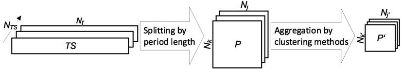
Figure 2. All N_{𝒯 𝒮} original time series 𝒯 𝒮 (left) with N_t time steps each are splitted into N_k periods 𝒫 (middle) with a period length of N_j segments each. Each period 𝒫 still consists of N_k⋅N_j = N_t time steps. Time-series aggregation to ${\mathit{\text{N}}}_{\mathit{\text{k}}\prime }$ typical periods 𝒫′ (right) with ${\mathit{\text{N}}}_{\mathit{\text{j}}\prime }$ segments in each typical period, i.e., number of time steps reduced to ${\mathit{\text{N}}}_{\mathit{\text{t}}\prime }={\mathit{\text{N}}}_{\mathit{\text{k}}\prime }\cdot {\mathit{\text{N}}}_{\mathit{\text{j}}\prime }\ll {\mathit{\text{N}}}_{\mathit{\text{t}}}$.

2.2. Aggregation of Periods to Typical Periods

Splitting of the time series 𝒯 𝒮 (Section 2.1) does not change the problem size (Figure 2: middle). The resulting N_k periods 𝒫 with N_j segments in each period still correspond to N_j⋅N_k = N_t = |𝒯𝒮| time steps of the original problem. In this section, we reduce the problem size by time-series aggregation to typical periods $\mathcal{P}\prime =\left\{{Ė}_{t\prime },{\text{c}}_{n,t\prime }^{\text{o}},\dots |t\prime \in \mathcal{T}\prime \right\}$ defined for a small set of time steps $|\mathcal{T}\prime |=N_{t\prime }\ll N_t$ (Figure 2: right). All periods consist of chronological time steps. The proposed method for time-series aggregation maintains chronology within each period; however, no chronology between periods is considered, and thus seasonal storage cannot be represented. To account for seasonal storage, a second time grid could be introduced as proposed by Renaldi and Friedrich (2017). Quite recently, Gabrielli et al. (2017) and Kotzur et al. (2017) considered seasonal storage in a synthesis problem by introduction of a second time grid to describe the sequence of typical periods, these authors further improved the approach of Renaldi and Friedrich (2017) by assigning all continuous variables to the full time horizon, while only the binary variables are considered for the sequence of aggregated typical periods.

In contrast to our previous work on non-chronological time series (Bahl et al., 2017a), typical periods allow aggregation in following two dimensions:

• N_k: the number of periods and

• N_j: the number of segments per period.

In the proposed method, first, the number of periods is aggregated (Section 2.2.1); subsequently, we aggregate the number of segments in each typical period (Section 2.2.2). This order was also applied by Fazlollahi et al. (2014). In this way, we can identify aggregated segments for each typical period individually, which is not possible if segments are aggregated first. In a preliminary version of the method (Bahl et al., 2017b), segments were aggregated first.

The aggregation is performed for a given number of typical periods $N_{k\prime }$ and aggregated segments $N_{j\prime }$. The overall method (Figure 1) then iteratively refines the number of typical periods and aggregated segments, for details see Section 2.4.

2.2.1. Aggregation of Number of Periods

The aggregation of N_k periods to $N_{k\prime }$ typical periods is based on clustering methods. Clustering aggregates the number of periods N_k while the number of segments N_j is invariant.

Clustering methods group data points from a (large) set of data into clusters. All data points in a cluster are represented by one cluster center (Jain et al., 1999). Here, we employ k-medoids as clustering method (Kaufman and Rousseeuw, 1987). The k-means clustering method (Lloyd, 1982) was also tested, and the impact of choice was small. This finding is in line with Schütz et al. (2016), showing that k-medoids leads to slightly better results than k-means.

For time-series aggregation to typical periods, one data point corresponds to a period p ∈ 𝒫, and each period p consists of N_j segments (Figure 3: top). In total, we have N_k periods p before the aggregation. By applying k-medoids clustering, we obtain $N_{k\prime }$ cluster centers representing the typical periods p′ ∈ 𝒫′ (Figure 3: middle). The share of the typical period p′ per year is determined by the number of periods p assigned to each typical period p′ (Figure 3). For multiple time series N_{𝒯 𝒮} > 1, each period p (and p′) corresponds to a vector of $N_{\mathcal{T}\mathcal{S}}\cdot N_j\left(N_{j\prime }\right)$ elements, thus the data of all time series are considered simultaneously in the clustering algorithm.

FIGURE 3

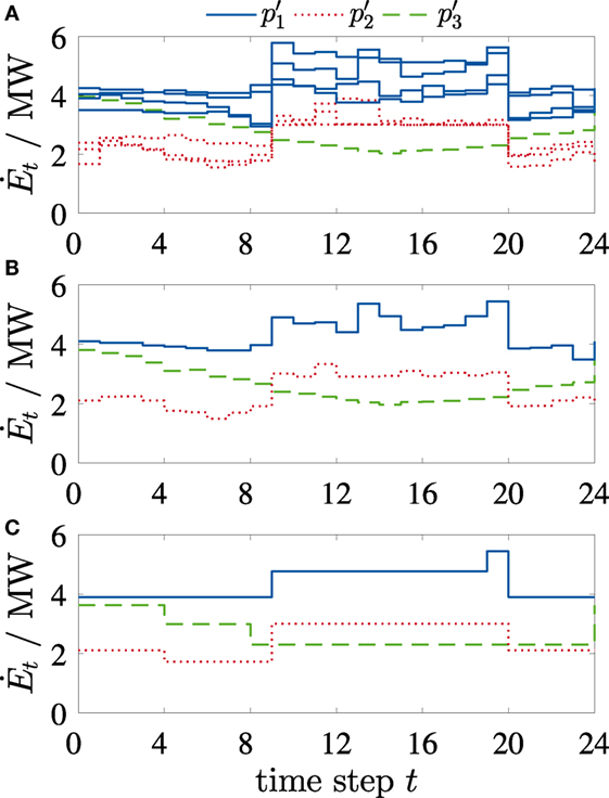
Figure 3. Illustrative time-series aggregation of N_{𝒯 𝒮} = 1 time series of an energy demand ${\dot{\mathit{\text{E}}}}_{\mathit{\text{t}}}$ with N_t = 216 time steps: (A) time-series splitted in N_k = 8 periods 𝒫 with N_j = 24 segments each. (B) Aggregation of periods 𝒫 to ${\mathit{\text{N}}}_{\mathit{\text{k}}\prime }=3$ typical periods 𝒫′. (C) Aggregation of N_j = 24 segments to ${\mathit{\text{N}}}_{\mathit{\text{j}}\prime }=3$ segments per typical period; segments do not start/end at 0 h. The line style of the periods in (A) indicates the clustering assignment to the typical periods ${\mathit{\text{p}}\prime }_1,{\mathit{\text{p}}\prime }_2,{\text{and}p\prime }_3$ in panels (B,C).

Mathematically, the clustering of periods to typical periods is an optimization problem minimizing the Euclidean distance dist(p, p′) between the cluster members and the cluster center:

$\begin{array}{ll}\hfill {\displaystyle \underset{p_k^{\prime },z_{i,k}}{\text{min}}}& {\displaystyle \sum _{i=1}^{N_k}}{\displaystyle \sum _{k=1}^{N_{k\prime }}}\text{\hspace{0.17em}dist\hspace{0.17em}}\left(p_i,p_k^{\prime }\right)\cdot z_{i,k},\end{array}$ (8)

$\begin{array}{ll}\hfill \text{s}.\text{t}.& {\displaystyle \sum _{k=1}^{N_{k\prime }}}{z}_{i,k}=1,\forall i\in \left[1,\dots ,N_k\right].\end{array}$

The assignment of a period p_i to a typical period p′_k results in the assignment matrix z_i,k. Typical periods p′_k are selected among existing periods p_i, thus, p′_k represents a real period (in contrast to the k-means clustering method, which would result in averaged, artificial periods). We use the PAM algorithm (Kaufman and Rousseeuw, 2008) with initialization of k-means++ (Arthur and Vassilvitskii, 2007) for solving the k-medoids problem in equation (8). By applying k-medoids, the yearly integral of the time series parameters in 𝒫′ and 𝒫 is not the same. For correction, we calculate a scaling factor for each time series separately (according to Domínguez-Muñoz et al. (2011)). The scaling factor is the ratio between the integral of all periods and the integral of all typical periods. All values of the typical periods p′ ∈ 𝒫′ are multiplied with the scaling factor for the corresponding time series to obtain the same integral values as with the original periods.

2.2.2. Aggregation of Number of Segments per Typical Period

The aggregated typical periods still contain the original number N_j of time steps per period. To aggregate the N_j time steps to N_j′ aggregated segments in a typical period (Figure 3C), a novel segment-clustering algorithm is proposed. A segment represents a group of consecutive time steps in a typical period. The segment-clustering algorithm maintains chronology between the segments in each typical period. Standard clustering algorithms like the Lloyd algorithm for k-means (Lloyd, 1982) and the PAM algorithm for k-medoids (Kaufman and Rousseeuw, 2008) used for period aggregation in Section 2.2.1 are not applicable: Standard clustering algorithms cannot consider a chronological coupling between the data points. If we want to aggregate the time steps in a period with 24 segments, a standard clustering algorithm interprets the time steps as 24 independent data points. Thus, the clustering algorithm results in, e.g., 4 clustered segments in this period without any information on the link between the segments—the chronology is lost.

The proposed segment-clustering algorithm minimizes the Euclidean distance between the aggregated segments and the original time steps in each typical period. Motivated by the Lloyd and PAM algorithms, we propose the following iterative procedure to minimize the Euclidean distance:

1. Initialize the clustering by splitting each typical period into a randomized segmentation with N_j′ segments.

2. For each segment, calculate the average value of the assigned time steps.

3. Assign the time steps at the end of a segment to the neighboring segment, if the value of the time step is closer to the average of the neighboring segment. Update the average value of the segment.

4. Repeat the reassignment of the ends of all segments in all typical periods until the assignment does not change or a maximum number of iterations are reached.

5. Repeat the procedure for multiple initial segmentations. Initializations can be obtained by Latin-hypercube sampling (McKay et al., 2000).

6. Considering the results from all initializations, use the aggregated segments with the smallest Euclidean distance to the original time steps.

The proposed segment-clustering algorithm is a heuristic, thus identifies local optima only. In step 5, multiple initializations are used to partly relieve this shortcoming. Different initializations might result in different local optima. In step 6, the “best” local optimum is selected among all identified local optima; however, this is still not guaranteed to be a global optimum.

The proposed segment-clustering algorithm has the advantage that any starting point can be used for a segment (c.f., Figure 3C). Thus, e.g., for N_j′ = 2, a separation in a “day” segment and a “night” segment is possible. Otherwise, if we split an annual time series with a start time at 12:00 a.m. at first of January into typical periods, 12:00 a.m. would be fixed as starting point of every first segment in a period. With a fixed starting point of the first segment at 12:00 a.m., we would need N_j′ = 3 segments to represent the day-night change by a “midnight-to-morning,” a “daytime” and an “evening-to-midnight” segment.

In this method, the time steps can be aggregated to any number of segments N_j. In the preliminary version of this method (Bahl et al., 2017b), segment-clustering was performed using equidistant segments in each period. Thus, the number of aggregated segments N_j′ had to be selected among the dividers of the period length N_j. Moreover, in the preliminary version, the starting point of the first segment was fixed to 12:00 a.m. For comparison, results of the case study in Section 3 using this preliminary version of the segment-clustering algorithm are presented in Supplementary Material.

The proposed segment-clustering algorithm belongs to the class of partitional clustering algorithms (Jain, 2010). In contrast, hierarchical clustering algorithms allocate the N_j′segments successively. For hierarchical clustering methods, the consideration of any starting point for the first segment is not directly realizable, as the segments are successively allocated (Jain, 2010).

Using the time-series aggregation (Sections 2.2.1 and 2.2.2), we obtain typical periods with individual aggregated segments in each typical period. The size of the typical periods 𝒫′ is significantly smaller than the size of the original time series (Figure 2: right):

$N_{k\prime }\cdot N_{j\prime }=N_{t\prime }\ll N_t.$ (9)

The resulting typical periods 𝒫′ are used for the synthesis problem in Section 2.3. After the solution of the synthesis problem, the accuracy of the aggregation is evaluated as an error in the domain of the objective function. If the time-series aggregation does not satisfy a required accuracy, the resolution of the typical periods is increased and the aggregation is restarted (Section 2.4).

In this article, the proposed time-series aggregation to typical periods is used for two-stage synthesis of energy systems. However, other applications of the time-series aggregation method are possible, e.g., simulation studies or scheduling of batch plants.

2.3. Solution of Optimization Problems

Using the typical periods 𝒫′ obtained from time-series aggregation in Section 2.2, we reduce the original synthesis problem (equations (2)–(6)) by solving the aggregated synthesis problem for the small set of time steps 𝒯′:

$\underset{{\dot{V}}_{n,t\prime },{\delta }_{n,t\prime },{\dot{V}}_n^{\text{N}},{\mathrm{\gamma }}_n,x}{\text{min}}{\displaystyle \sum _{t\prime \in \mathcal{T}\prime }}\left(\mathrm{\Delta }{\text{t}}_{t\prime }{\displaystyle \sum _{n\in \mathcal{C}}}{\text{c}}_{n,t\prime }^{\text{o}}\frac{{\dot{V}}_{n,t\prime }}{{\eta }_n}\right)+\frac{1}{\mathit{\text{APVF}}}{\displaystyle \sum _{n\in \mathcal{C}}}{\text{c}}_n^{\text{i}}{\dot{V}}_n^{\text{N}},$ (10)

$\begin{array}{ll}\hfill \text{s}.\text{t}.{\displaystyle \sum _{n\in \mathcal{C}}}{\dot{V}}_{n,t\prime }& ={Ė}_{t\prime },\forall t\prime \in \mathcal{T}\prime ,\end{array}$ (11)

$\begin{array}{l}\hfill A_1^{\prime }{\dot{V}}_{n,t\prime }+{\tilde{A}}_1^{\prime }{\delta }_{n,t\prime }\le b_1,\forall t\prime \in \mathcal{T}\prime ,\forall n\in \mathcal{C},\end{array}$ (12)

$\begin{array}{l}\hfill A_2{\dot{V}}_n^{\text{N}}+{\tilde{A}}_2{\mathrm{\gamma }}_n\le b_2,\forall n\in \mathcal{C},\end{array}$ (13)

$\begin{array}{l}\hfill A_3^{\prime }{\left({\dot{V}}_{n,t\prime },{\delta }_{n,t\prime },{\dot{V}}_n^{\text{N}},{\mathrm{\gamma }}_n,x\right)}^{\text{T}}\le b_3.\end{array}$ (14)

${\dot{V}}_{n,t\prime }\in {\mathbb{R}}^{+},{\dot{V}}_n^{\text{N}}\in {\mathbb{R}}^{+},{\delta }_{n,t\prime }\in \left\{0,1\right\},{\mathrm{\gamma }}_n\in \left\{0,1\right\},x\in {\mathbb{R}}^a\times {\left\{0,1\right\}}^{\tilde{a}}.$

This aggregated synthesis problem (equations (10)–(14)) is identical to the original synthesis problem (equations (2)–(6)), but stated for t′ ∈ 𝒯′. Thereby, time-series aggregation enables an efficient solution as the large operation decision vector $\left({\dot{V}}_{n,t},{\delta }_{n,t}\right)$ is aggregated to $\left({\dot{V}}_{n,t\prime },{\delta }_{n,t\prime }\right)$ with $\mathrm{|}{\dot{V}}_{n,t\prime }\mathrm{|}\ll \mathrm{|}{\dot{V}}_{n,t}\mathrm{|}$ and $\mathrm{|}{\delta }_{n,t\prime }\mathrm{|}\ll \mathrm{|}{\delta }_{n,t}\mathrm{|}$. The optimization yields the optimal structure $\left({\dot{V}}_n^{\text{N}\ast },{\mathrm{\gamma }}_n^{\ast }\right)$ as solution of the aggregated synthesis problem with the objective function value total annualized cost ${\mathit{\text{TAC}}}^{\ast }\left(\mathcal{P}\prime \right):=\mathit{\text{TAC}}\left({\dot{V}}_n^{\text{N}\ast },{\mathrm{\gamma }}_n^{\ast },{\dot{V}}_{n,t\prime }^{\ast },{\delta }_{n,t\prime }^{\ast }\right)$. However, the solution is only optimal for the aggregated typical periods 𝒫′.

To evaluate the accuracy of the aggregation, the structure $\left({\dot{V}}_n^{\text{N}\ast },{\mathrm{\gamma }}_n^{\ast }\right)$ is subsequently used to solve an operation problem for the complete time series 𝒯 𝒮 and the complete operation decision vector $\left({\dot{V}}_{n,t},{\delta }_{n,t}\right)$:

$\underset{{\dot{V}}_{n,t},{\delta }_{n,t},x}{\text{min}}{\displaystyle \sum _{t\in \mathcal{T}}}\left(\mathrm{\Delta }{\text{t}}_t{\displaystyle \sum _{n\in \mathcal{C}}}{\text{c}}_{n,t}^{\text{o}}\frac{{\dot{V}}_{n,t}}{{\eta }_n}\right)+\frac{1}{\mathit{\text{APVF}}}{\displaystyle \sum _{n\in \mathcal{C}}}{\text{c}}_n^{\text{i}}{\dot{V}}_n^{\text{N}\ast },$ (15)

$\begin{array}{l}\hfill \text{s}.\text{t}.{\displaystyle \sum _{n\in \mathcal{C}}}{\dot{V}}_{n,t}={Ė}_t,\forall t\in \mathcal{T},\end{array}$ (16)

$\begin{array}{l}\hfill A_1{\dot{V}}_{n,t}+{\tilde{A}}_1{\delta }_{n,t}\le b_1,\forall t\in \mathcal{T},\forall n\in \mathcal{C},\end{array}$ (17)

$\begin{array}{l}\hfill A_3{\left({\dot{V}}_{n,t},{\delta }_{n,t},{\dot{V}}_n^{\text{N}\ast },{\mathrm{\gamma }}_n^{\ast },x\right)}^{\text{T}}\le b_3.\end{array}$ (18)

$\begin{array}{ll}\hfill {\dot{V}}_{n,t}\in {\mathbb{R}}^{+},{\delta }_{n,t}\in \left\{0,1\right\},x& \in {\mathbb{R}}^a\times {\left\{0,1\right\}}^{\tilde{a}}.\end{array}$

The feasibility of the structure $\left({\dot{V}}_n^{\text{N}\ast },{\mathrm{\gamma }}_n^{\ast }\right)$ in the operation problem with the complete time series 𝒯 𝒮 cannot be guaranteed. Thus, we iteratively add so-called feasibility time steps (Bahl et al., 2017a) to ensure feasibility of structure $\left({\dot{V}}_n^{\text{N}\ast },{\mathrm{\gamma }}_n^{\ast }\right)$. Aggregation always involves averaging and thus neglects extreme conditions of the full time series. To circumvent this shortcoming, additional peak demands are commonly considered in aggregation methods (Mavrotas et al., 2008; Domínguez-Muñoz et al., 2011; Ortiga et al., 2011; Voll et al., 2013; Fazlollahi et al., 2014; Bungener et al., 2015; Lythcke-Jøgensen et al., 2016). In contrast to typical periods, these peak demands are single time steps with a duration $\mathrm{\Delta }{t}_t$ of zero and without any chronological order to other time steps. Thus, the energy system needs to supply these peak demands without storage and consideration of time-coupling constraints. Thus, besides the typical periods, we consider peak demands as feasibility time steps in the aggregated synthesis problem (equations (10)–(14)). However, even when we consider peak demands as feasibility time steps, operation can still be infeasible (Bahl et al., 2017a). If the operation problem fails, we iteratively add additional feasibility time steps. We add the infeasible time step with maximum heating (odd iteration) or cooling demand (even iteration) as new feasibility time step. If the structure $\left({\dot{V}}_n^{\text{N}\ast },{\mathrm{\gamma }}_n^{\ast }\right)$ is feasible for the operation problem with the full time series 𝒯 𝒮 (equations (15)–(18)), we obtain the solution $\left({\dot{V}}_{n,t}^{\ast },{\delta }_{n,t}^{\ast }\right)$ with objective function value ${\mathit{\text{TAC}}}^{\ast }\left(\mathcal{T}\mathcal{S}\right):=\mathit{\text{TAC}}\left({\dot{V}}_n^{\text{N}\ast },{\mathrm{\gamma }}_n^{\ast },{\dot{V}}_{n,t}^{\ast },{\delta }_{n,t}^{\ast }\right)$.

Using the results from the operation problem, the accuracy of the time-series aggregation is calculated to evaluate the quality of the solution obtained in the aggregated synthesis problem.

2.4. Evaluation of Accuracy and Increasing Resolution of Typical Periods

After solving the operation problem, we measure the accuracy of aggregation in the domain of the objective function (here: total annualized cost TAC) as proposed by Bahl et al. (2017a) for synthesis problems without chronological time steps. The accuracy measure ΔTAC is calculated as the difference of the optimal objective function values between the aggregated synthesis problem TAC*(𝒫′) and the operation problem with the complete time series ${\mathit{\text{TAC}}}^{\ast }\left(\mathcal{T}\mathcal{S}\right)$:

$\begin{array}{ll}\hfill \mathrm{\Delta }\mathit{\text{TAC}}& =\left|{\mathit{\text{TAC}}}^{\ast }\left(\mathcal{P}\prime \right)-{\mathit{\text{TAC}}}^{\ast }\left(\mathcal{T}\mathcal{S}\right)\right|\\ \hfill & =\left|{\mathit{\text{OPEX}}}^{\ast }\left(\mathcal{P}\prime \right)-{\mathit{\text{OPEX}}}^{\ast }\left(\mathcal{T}\mathcal{S}\right)\right|.\end{array}$ (19)

The structure $\left({\dot{V}}_n^{\text{N}\ast },{\mathrm{\gamma }}_n^{\ast }\right)$—and thus the investment cost CAPEX—is fixed for the operation problem. Hence, the difference of TAC results in a difference of the operational expenditure OPEX. The accuracy of time-series aggregation ΔTAC is evaluated against a threshold value ϵ:

$\mathrm{\Delta }\mathit{\text{TAC}}\le \mathrm{ϵ}.$ (20)

This threshold value ϵ can be set, e.g., equal to the optimality gap ϵ_Syn of the synthesis problem as the accuracy is measured in the objective function domain. If a relative optimality gap is set in the synthesis problem, the accuracy measure ΔTAC in equation (20) needs to be normalized by $\mathit{\text{TA}}{C}^{\ast }\left(\mathcal{P}\prime \right)$.

If the accuracy criterion equation (20) is not met, the resolution of the typical periods 𝒫′ is increased. The resolution can be increased by a higher number of typical periods $N_{k\prime }$ or a higher number of segments $N_{j\prime }$. These numbers span a grid $\left(N_{k\prime }\times N_{j\prime }\right)$ of possible resolutions $\left(N_{k\prime },N_{j\prime }\right)$ for typical periods 𝒫′. In this grid, we select a higher resolution based on earlier improvements for resolving either direction. More formally, we compare finite backward differences ∇TAC_k and ∇TAC_j:

$\begin{array}{ll}\hfill \nabla {\mathit{\text{TAC}}}_k& =\mathrm{\Delta }\text{TAC}\left({\text{GP}}_k\right)-\mathrm{\Delta }\mathit{\text{TAC}}\left(N_{k\prime },N_{j\prime }\right),\end{array}$ (21)

$\begin{array}{ll}\hfill \nabla {\mathit{\text{TAC}}}_j& =\mathrm{\Delta }\mathit{\text{TAC}}\left({\mathit{\text{GP}}}_j\right)-\mathrm{\Delta }\mathit{\text{TAC}}\left(N_{k\prime },N_{j\prime }\right).\end{array}$ (22)

We calculate the backward differences ∇TAC_k, ∇TAC_j between the accuracy ΔTAC of the current grid point $\left(N_{k\prime },N_{j\prime }\right)$ and the accuracy ΔTAC of previously calculated grid points,

$\begin{array}{ll}\hfill {\mathit{\text{GP}}}_k& =\left(N_{k\prime }-1,\widetilde{N_{j\prime }}\right),\end{array}$ (23)

$\begin{array}{ll}\hfill {\mathit{\text{GP}}}_j& =\left(\widetilde{N_{k\prime }},N_{j\prime }-1\right).\end{array}$ (24)

The grid point GP_k is always at $N_{k\prime }-1$ coordinate. The coordinate $\widetilde{N_{j\prime }}$ corresponds to the last known grid point at $N_{k\prime }-1$. Most likely this is $N_{j\prime }$, but it can also be $N_{j\prime }-1,N_{j\prime }-2,...$—depending on the history of the current run. The grid point GP_j is formed accordingly. The grid points (GP_k, GP_j) are stored during previous iterations. Based on the backward differences ∇TAC_k, ∇TAC_j in equations (21) and (22), the resolution is increased by increasing either $N_{k\prime }$ or $N_{j\prime }$:

• If the backward difference for the number of typical periods is larger (∇TAC_k ≥ ∇TAC_j), we store the grid point ${\mathit{\text{GP}}}_k=\left(N_{k\prime },N_{j\prime }\right)$ and refine the number of periods $N_{k\prime }=N_{k\prime }+1$.

• Otherwise, the backward difference for the number of segments is larger (∇TAC_k < ∇TAC_j), and we store the grid point ${\mathit{\text{GP}}}_j=\left(N_{k\prime },N_{j\prime }\right)$ and refine the number of segments $N_{j\prime }=N_{j\prime }+1$.

The refined resolution $\left(N_{k\prime },N_{j\prime }\right)$ is used to restart the aggregation to new typical periods 𝒫′. For the first iterations, no previous grid points are available, and we initialize the method (Figure 1) with:

1. Set: $N_{k\prime }=1$, $N_{j\prime }=2$, evaluate accuracy ΔTAC(1,2), store GP_k = (1,2),

2. Set: $N_{k\prime }=2$, $N_{j\prime }=1$, evaluate accuracy ΔTAC(2,1), store GP_j = (2,1).

After two initial calculations, we know the accuracy ΔTAC of the grid points GP_k = (1,2) and GP_j = (2,1). For the third iteration $\left(N_{k\prime }=2,N_{j\prime }=2\right)$ and further iterations, we calculate backward differences ∇TAC_k and ∇TAC_j (equations (21) and (22)). We iteratively increase the resolution of the typical periods 𝒫′ until the accuracy criterion equation (20) is met and the solution for synthesis decision $\left({\dot{V}}_n^{\text{N}\ast },{\mathrm{\gamma }}_n^{\ast }\right)$ satisfies the required accuracy ϵ = ϵ_Syn. In the following, the method is applied to a real-world case study.

3. Real-World Case Study

The presented method is applied to a real-world case study based on Voll et al. (2013). We extend the case study by introduction of thermal storage and volatile electricity prices. In Section 3.1, the synthesis problem is described, the time series are presented, and benchmark periods are defined. The results of the proposed time-series aggregation method are discussed in Section 3.2.

3.1. Problem Description

The superstructure of the considered energy supply system consists of multiple units of boilers (B), combined heat and power engines (CHP), absorption chillers (AC), and compression chillers (CC) (Figure 4). We extend the superstructure by thermal storage (ST) units for cooling and heating. The model allows continuous sizing of all units. Constant part-load efficiency is assumed for all units. Details of the mixed-integer linear model are presented in the Supplementary Material. We consider an original time series with a resolution of 1 h for heating, cooling, and electricity demand (Figure 5A) as well as for volatile electricity purchase and selling price (Figure 5B). The synthesis problem with this original time series is referred to as original instance. For the computational study, we generate 10 instances from the data of the original instance using Latin-hypercube sampling (McKay et al., 2000) with a variation of the time series of ±5%.

FIGURE 4

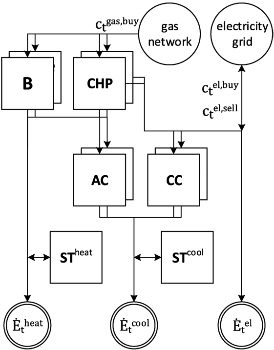
Figure 4. Superstructure of real-world example based on Voll et al. (2013): boiler (B), combined heat and power unit (CHP), compression chiller (CC), and absorption chiller (AC) extended by thermal storage (ST) with variable capacity for cooling and heating. Time series (Figure 5) of volatile energy prices c_t and energy demands ${\dot{\mathit{\text{E}}}}_{\mathit{\text{t}}}$ are considered.

FIGURE 5

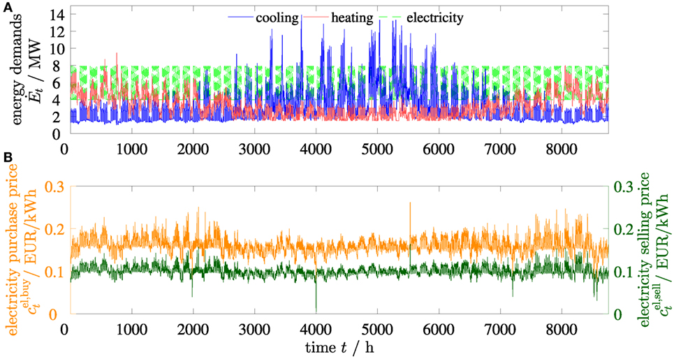
Figure 5. Time series 𝒯 𝒮 of the original instance for (A) heating, cooling, and electricity demands, and (B) electricity purchase and selling price over 1 year with a resolution of 1 h.

All calculations are performed using 4 Intel-Xeon CPUs with 3.0 GHz and 64 GB memory. All MILP problems are solved using CPLEX 12.6.3.0 (IBM Corporation, 2015) with a time limit of 1 h, which is not reached by the calculations. We set the optimization gap of the synthesis problem to ϵ_Syn = 2% and accordingly the threshold value of the time-series aggregation method to ϵ = ϵ_Syn = 2%.

The proposed time-series aggregation to typical periods is compared with benchmark periods. The benchmark periods are based on an intuitive selection of existing days of the original time series: for $N_{k\prime }=1$, we selected an arbitrary spring day, for $N_{k\prime }=2$ we selected a arbitrary summer and winter day, for $N_{k\prime }=4$ we selected one arbitrary day per season, for $N_{k\prime }=6$ we selected one arbitrary day in every second month, and for $N_{k\prime }=12$ we selected one arbitrary day per month. Moreover, for $N_{k\prime }=6$, we select typical days according to VDI 4655 standard of selection representative load profiles (The Association of German Engineers, 2008). The calculation of the accuracy of the benchmark periods is identical to the accuracy measure in the proposed method.

3.2. Results

In this section, we present results of the proposed method for the real-world case study. After the presolve by CPLEX, the original synthesis problem (equations (2)–(6)) with the full time-series data (Figure 5) has 1,428,000 constraints, 692,000 variables (including 202,000 binary variables), and 3,566,000 non-zero elements. As benchmark, we solve the original synthesis problem with CPLEX directly. The solution results in an optimality gap of 12% after 96 h. The best feasible solution provided by the benchmark with CPLEX has total annualized cost of 8.08 Mio. €. The proposed time-series aggregation method (Section 2) yields a feasible solution for the original synthesis problem with total annualized cost of 7.16 Mio. € after 15 min. In the following sections, detailed results of the time-series aggregation method are discussed.

First, we discuss results of the autocorrelation to identify the period length in Section 3.2.1. In Section 3.2.2, the accuracy of the time-series aggregation is evaluated depending on the resolution of the typical periods 𝒫′. Finally, in Section 3.2.3, the proposed k-medoids-based aggregation is compared with typical periods based on intuitive selection and VDI 4655.

3.2.1. Period Length

The period length is identified by analyzing the normalized sum of autocorrelation functions calculated according to equation (7). The peaks in Figure 6 indicate a period length of 24 and 168 h corresponding to 1 day and 1 week. By time-series aggregation, we aim at reducing the problem size of the synthesis problem. Thus, we favor short periods and select N_j = 24 h as period length. If it is impossible to reach the threshold ϵ, we go back to the period length selection and choose a week as period length.

FIGURE 6

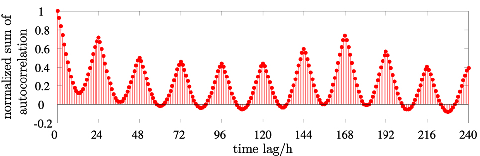
Figure 6. Normalized sum of autocorrelation function (equation (7)) with a time lag of 0–240 h.

3.2.2. Accuracy of Aggregated Synthesis Problem

With the identified period length of 24 h, we start the iterative aggregation of typical periods. The calculations are performed for the original instance and the 10 generated instances. For the original instance (Figure 7: circles), we identify that $N_{k\prime }=2$ typical periods and $N_{j\prime }=2$ segments are required to obtain a solution with a smaller error than the threshold ΔTAC < ϵ, equation (19). Thus, in total 6 time steps (4 time steps of the typical periods plus 2 feasibility time steps) are required to represent the cost of the full time series of 8,760 time steps with excellent accuracy. All 10 generated instances of the computational study (Figure 7: squares) show a similar behavior and 4–12 time steps are sufficient to meet the required threshold ϵ = 2%. Thus, for synthesis problems with the requirement of chronological time steps, few typical periods with few segments per typical period are sufficient to represent the complete time series with small error in the objective function. Time-series aggregation reduces the number of time steps and thus the size of the synthesis problem by a factor of 1,000.

FIGURE 7

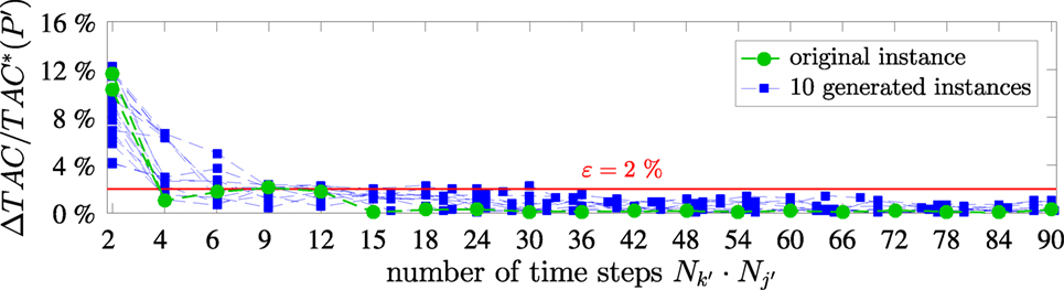
Figure 7. Normalized accuracy measure ΔTAC divided by total annualized cost of the aggregated synthesis problem TAC*(𝒫′) as function of number of time steps $\left({\mathit{\text{N}}}_{\mathit{\text{k}}\prime }\cdot {\mathit{\text{N}}}_{\mathit{\text{j}}\prime }\right)$ for the original instance and 10 generated instances, threshold value of ϵ = 2% as solid red line.

Infeasibility of the structure $\left({\dot{V}}_n^{\text{N}\ast },{\mathrm{\gamma }}_n^{\ast }\right)$ for the operation problem (Section 2.3) occurs less often than in a synthesis problem without the consideration of storage (Bahl et al., 2017a). This is expected because storage can compensate some infeasibilities. However, feasibility of $\left({\dot{V}}_n^{\text{N}\ast },{\mathrm{\gamma }}_n^{\ast }\right)$ is still not guaranteed by aggregated time series with additional peak demands, and adding further feasibility time steps in the method is still required: considering all instances of the computational study, we find that infeasibility of the operation problem occurs in 12 of all 305 calculations (i.e., 4%), if only peak demands are considered as feasibility time steps.

In the proposed method, we increase the number of typical periods $N_{k\prime }$ or the number of segments $N_{j\prime }$ based on finite backward differences (Section 2.4). To assess the efficiency of this heuristic strategy, we calculate the complete grid of $N_{k\prime }\times N_{j\prime }$ for the original instance (Figure 8). The proposed method identifies the minimal number of 4 time steps to satisfy the threshold value: ΔTAC = 1% < ϵ = 2% (Figure 8: bold numbers). Moreover, we observe that generally few typical periods $N_{k\prime }$ with few segments $N_{j\prime }$ satisfy the threshold value ϵ in a wide range of possible combinations (Figure 8: dark green areas).

FIGURE 8

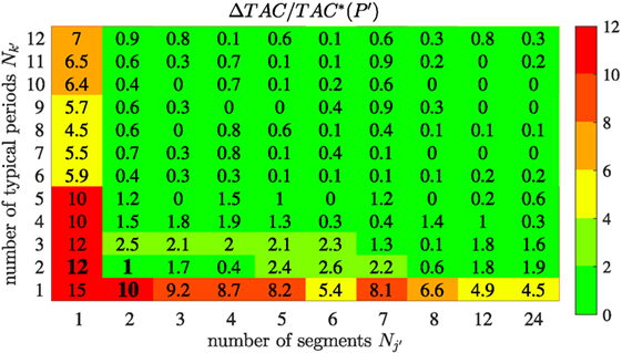
Figure 8. Normalized accuracy measure ΔTAC divided by total annualized cost of the aggregated synthesis problem TAC*(𝒫′) in percent as numbers in the cells and color code. The path of the iterative method is indicated with bold numbers.

In general, the increased resolution of time-series aggregation (Section 2.4) will propagate from the lower left corner (low accuracy) to the upper right corner (high accuracy). In the original instance (Figure 8), the heuristic based on backward differences identifies the global minimal number of time steps satisfying the threshold value. In other instances of the computational study, the heuristic selection cannot guarantee that the minimal number of time steps is found. In Table 1, the minimal number of time steps identified by the method is compared with the minimal number based on a calculation of the complete grid for all instances. In 64% of all instances, the number identified by the method is equal to the minimal number possible considering the complete grid. However, in one instance the minimal number of time steps identified by the method is 3 times higher than the actual minimum. Thus, the heuristic generally does not guarantee the minimal number of time steps, but based on the finite backward differences a small number of total time steps is identified and very good solutions are found.

TABLE 1

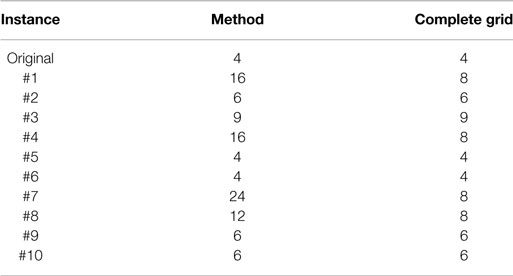
Table 1. Minimal number of time steps identified by the method and considering the complete grid.

3.2.3. Comparison of Selected Typical Periods to Benchmark Periods

The proposed time-series aggregation method is compared with typical periods obtained by an intuitive selection introduced in Section 3.1 and typical periods based on VDI 4655. For this comparison, the number of segments per typical period is fixed to $N_{j\prime }=24$ (rightmost column in Figure 8) since this is the resolution employed by VDI 4655. The benchmark periods are evaluated with the same accuracy criterion as proposed in the time-series aggregation method (Section 2.4), only the clustering-based aggregation is replaced (Section 2.2).

The proposed time-series aggregation method shows higher accuracy than the benchmark typical periods (Figure 9). 12 typical benchmark periods have a similar accuracy as 1 typical period obtained by the proposed time-series aggregation method. In this example, for $N_{k\prime }=6$, the typical periods based on VDI 4655 show the lowest accuracy but are in the same range as the intuitive days. In contrast, the proposed time-series aggregation method quickly reduces the error of aggregation in the domain of the objective function (Figure 9: circles) when the number of periods is increased: only 2 typical periods obtained by the proposed time-series aggregation method already satisfy the defined threshold, while the intuitive selection (Figure 9: squares) does not satisfy the defined threshold with the maximum considered number of 12 typical periods.

FIGURE 9

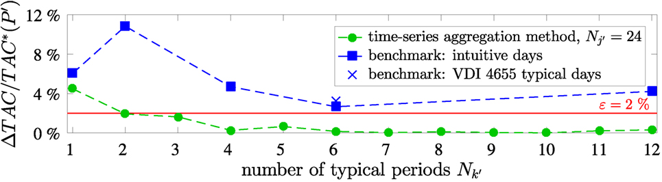
Figure 9. Normalized accuracy measure ΔTAC divided by total annualized cost of the aggregated synthesis problem TAC*(𝒫′) as function of number of typical periods ${\mathit{\text{N}}}_{\mathit{\text{k}}\prime }$ with N_j = 24 segments. Benchmark periods based on intuitive selection of typical periods (N_k = 1: spring day, N_k = 2: summer and winter day, N_k = 4: 1 day per season, N_k = 6: 1 day for every second month, and N_k = 12: 1 day per month) and selection of N_k = 6 typical days according to VDI 4655.

We want to point out that in our method (Section 2.2.2), we additionally aggregate the time steps in each typical period and find that $N_{j\prime }=2$ segments in the $N_{k\prime }=2$ typical periods are sufficient to satisfy the threshold (Figures 7 and 8). Thus, our aggregation method requires 4 time steps to satisfy the threshold value, while $12\cdot 24=288$ time steps of the benchmark typical periods are not sufficient.

4. Conclusion

Two-stage synthesis problems of real-world energy systems are often too complex to be solved in reasonable time or with available computer memory. In these cases, time-series aggregation can be employed to reduce the problem complexity. In many problems, time-series aggregation has to account for chronology, for example, if storage is considered in the energy system. Time-series aggregation to typical periods can account for chronological time steps.

We present an aggregation method to typical periods with aggregated segments for the synthesis of energy systems. The method bounds the error of aggregation not in the time-series domain, but in the domain of the objective function and thus captures the purpose of the optimization problem. The method is applied to an extended real-world case study based on Voll et al. (2013) with a test set of 10 instances of the time series.

In a first step of the method, we use autocorrelation to identify typical period lengths of 24 and 168 h proving an expected daily and weekly periodicity of the data using autocorrelation. The proposed method allows to reduce the problem size drastically: For the original instance, a time-series aggregation to 2 typical periods with 2 segments in each typical period plus 2 additional peak demand time steps already leads to a better accuracy of the cost of the energy system than required by the optimization gap of the synthesis problem. This corresponds to a reduction of the time steps in the synthesis problem (and thus the optimization problem size) by a factor of 1,000. The results also show that our time-series aggregation method based on clustering outperforms the accuracy of intuitive benchmark periods as well as VDI 4655-based results. We conclude that few typical periods with few segments per period are sufficient to represent the full time series accurately with small error in the (cost) objective function. The proposed time-series aggregation method efficiently identifies the few required typical periods to guarantee high quality energy system designs.

Author Contributions

All authors contributed substantially to the conception of the work and to its intellectual content and approved the final version.

Conflict of Interest Statement

The authors declare that the research was conducted in the absence of any commercial or financial relationships that could be construed as a potential conflict of interest.

The reviewer, SB, and handling Editor declared their shared affiliation.

Funding

This study is funded by the German Federal Ministry for Economic Affairs and Energy (ref. no.: 03ET1259A). The support is gratefully acknowledged.

Supplementary Material

The Supplementary Material for this article can be found online at http://www.frontiersin.org/articles/10.3389/fenrg.2017.00035/full#supplementary-material.

References

Al-Wakeel, A., Wu, J., and Jenkins, N. (2017). k-means based load estimation of domestic smart meter measurements. Appl. Energy 194, 333–342. doi: 10.1016/j.apenergy.2016.06.046

CrossRef Full Text | Google Scholar

Arthur, D., and Vassilvitskii, S. (2007). “k-means++: The advantages of careful seeding,” in Proceedings of the Eighteenth Annual ACM-SIAM Symposium on Discrete Algorithms, SODA ’07 (Philadelphia, PA, USA: Society for Industrial and Applied Mathematics), 1027–1035.

Google Scholar

Bahl, B., Kümpel, A., Lampe, M., and Bardow, A. (2017a). Time-series aggregation for synthesis problems by bounding error in the objective function. Energy 135, 900–912. doi:10.1016/j.energy.2017.06.082

CrossRef Full Text | Google Scholar

Bahl, B., Söhler, T., Hennen, M., and Bardow, A. (2017b). “Time-series aggregation to typical periods with bounded error in objective function for energy systems synthesis,” in Proceedings of ECOS 2017: 30th International Conference on Efficiency, Cost, Optimization, Simulation, and Environmental Impact of Energy Systems, San Diego, CA, 726–737.

Google Scholar

Biegler, L. T., Grossmann, I. E., and Westerberg, A. W. (1997). Systematic Methods of Chemical Process Design. Upper Saddle River, NJ: Prentice Hall PTR.

Google Scholar

Box, G. E., Jenkins, G. M., Reinsel, G. C., and Ljung, G. M. (2015). Autocorrelation Function and Spectrum of Stationary Processes, Chap. 2. Hoboken: John Wiley & Sons, 21–45.

Google Scholar

Bracco, S., Dentici, G., and Siri, S. (2016). DESOD: a mathematical programming tool to optimally design a distributed energy system. Energy 100, 298–309. doi:10.1016/j.energy.2016.01.050

CrossRef Full Text | Google Scholar

Brodrick, P. G., Kang, C. A., Brandt, A. R., and Durlofsky, L. J. (2015). Optimization of carbon-capture-enabled coal-gas-solar power generation. Energy 79, 149–162. doi:10.1016/j.energy.2014.11.003

CrossRef Full Text | Google Scholar

Bungener, S., Hackl, R., Eetvelde, G. V., Harvey, S., and Marechal, F. (2015). Multi-period analysis of heat integration measures in industrial clusters. Energy 93, 220–234. doi:10.1016/j.energy.2015.09.023

CrossRef Full Text | Google Scholar

Domínguez-Muñoz, F., Cejudo-López, J. M., Carrillo-Andrés, A., and Gallardo-Salazar, M. (2011). Selection of typical demand days for CHP optimization. Energ Build 43, 3036–3043. doi:10.1016/j.enbuild.2011.07.024

CrossRef Full Text | Google Scholar

European Commission. (2014). A Policy Framework for Climate and Energy in the Period from 2020 to 2030. Brussels: Communication from the Commission to the European Parliament, the Council, the European Economic and Social Committee and the Committee of the Regions.

Google Scholar

Fazlollahi, S., Bungener, S. L., Mandel, P., Becker, G., and Maréchal, F. (2014). Multi-objectives, multi-period optimization of district energy systems: I-selection of typical operating periods. Comput. Chem. Eng. 54–66. doi:10.1016/j.compchemeng.2014.03.005

CrossRef Full Text | Google Scholar

Fitiwi, D. Z., de Cuadra, F., Olmos, L., and Rivier, M. (2015). A new approach of clustering operational states for power network expansion planning problems dealing with RES (renewable energy source) generation operational variability and uncertainty. Energy 90, 1360–1376. doi:10.1016/j.energy.2015.06.078

CrossRef Full Text | Google Scholar

Gabrielli, P., Gazzani, M., Martelli, E., and Mazzotti, M. (2017). Optimal design of multi-energy systems with seasonal storage. Appl. Energy. 212:720. doi:10.1016/j.apenergy.2017.07.142

CrossRef Full Text | Google Scholar

Goderbauer, S., Bahl, B., Voll, P., Lübbecke, M. E., Bardow, A., and Koster, A. M. (2016). An adaptive discretization {MINLP} algorithm for optimal synthesis of decentralized energy supply systems. Comput. Chem. Eng. 95, 38–48. doi:10.1016/j.compchemeng.2016.09.008

CrossRef Full Text | Google Scholar

Green, R., Staffell, I., and Vasilakos, N. (2014). Divide and conquer? k-means clustering of demand data allows rapid and accurate simulations of the British electricity system. IEEE T Eng. Manage. 61, 251–260. doi:10.1109/TEM.2013.2284386

CrossRef Full Text | Google Scholar

Heuberger, C. F., Rubin, E. S., Staffell, I., Shah, N., and Dowell, N. M. (2017). Power capacity expansion planning considering endogenous technology cost learning. Appl. Energy 204(Suppl. C), 831–845. doi:10.1016/j.apenergy.2017.07.075

CrossRef Full Text | Google Scholar

IBM Corporation. (2015). IBM ILOG CPLEX Optimization Studio, Version 12.6. User Guide, Armonk.

Google Scholar

Jain, A. K. (2010). Data clustering: 50 years beyond k-means. Patt. Recog. Lett. 31, 651–666. doi:10.1016/j.patrec.2009.09.011

CrossRef Full Text | Google Scholar

Jain, A. K., Murty, M. N., and Flynn, P. J. (1999). Data clustering: a review. ACM Comput. Surv. 31, 264–323. doi:10.1145/331499.331504

CrossRef Full Text | Google Scholar

Kaufman, L., and Rousseeuw, P. (1987). Clustering by Means of Medoids. North-Holland: Reports of the Faculty of Mathematics and Informatics, 87.

Google Scholar

Kaufman, L., and Rousseeuw, P. J. (2008). Partitioning Around Medoids (Program PAM), Chap. 2. Hoboken: John Wiley & Sons Inc, 68–125.

Google Scholar

Kools, L., and Phillipson, F. (2016). Data granularity and the optimal planning of distributed generation. Energy 112, 342–352. doi:10.1016/j.energy.2016.06.089

CrossRef Full Text | Google Scholar

Kotzur, L., Markewitz, P., Robinius, M., and Stolten, D. (2017). Time Series Aggregation for Energy System Design: Modeling Seasonal Storage. arXiv:1710.07593 [math.OC]. Available from: https://arxiv.org/abs/1710.07593

Google Scholar

Lin, F., Leyffer, S., and Munson, T. (2016). A two-level approach to large mixed-integer programs with application to cogeneration in energy-efficient buildings. Comput. Optim. Appl. 65, 1–46. doi:10.1007/s10589-016-9842-0

CrossRef Full Text | Google Scholar

Lloyd, S. (1982). Least squares quantization in PCM. IEEE Trans. Inf. Theor. 28, 129–137. doi:10.1109/TIT.1982.1056489

CrossRef Full Text | Google Scholar

Lozano, M. A., Ramos, J. C., Carvalho, M., and Serra, L. M. (2009). Structure optimization of energy supply systems in tertiary sector buildings. Energy Build. 41, 1063–1075. doi:10.1016/j.enbuild.2009.05.008

CrossRef Full Text | Google Scholar

Lythcke-Jøgensen, C. E., Münster, M., Ensinas, A. V., and Haglind, F. (2016). A method for aggregating external operating conditions in multi-generation system optimization models. Appl. Energy 166, 59–75. doi:10.1016/j.apenergy.2015.12.050

CrossRef Full Text | Google Scholar

Mancarella, P. (2014). MES (multi-energy systems): an overview of concepts and evaluation models. Energy 65, 1–17. doi:10.1016/j.energy.2013.10.041

CrossRef Full Text | Google Scholar

Marton, C., Elkamel, A., and Duever, T. (2008). An order-specific clustering algorithm for the determination of representative demand curves. Comput. Chem. Eng. 32, 1365–1372. doi:10.1016/j.compchemeng.2007.06.010

CrossRef Full Text | Google Scholar

Mavrotas, G., Diakoulaki, D., Florios, K., and Georgiou, P. (2008). A mathematical programming framework for energy planning in services’ sector buildings under uncertainty in load demand: the case of a hospital in Athens. Energy Pol. 36, 2415–2429. doi:10.1016/j.enpol.2008.01.011

CrossRef Full Text | Google Scholar

McKay, M. D., Beckman, R. J., and Conover, W. J. (2000). A comparison of three methods for selecting values of input variables in the analysis of output from a computer code. Technometrics 42, 55–61. doi:10.1080/00401706.2000.10485979

CrossRef Full Text | Google Scholar

Nahmmacher, P., Schmid, E., Hirth, L., and Knopf, B. (2016). Carpe diem: a novel approach to select representative days for long-term power system modeling. Energy 112, 430–442. doi:10.1016/j.energy.2016.06.081

CrossRef Full Text | Google Scholar

Oluleye, G., Vasquez, L., Smith, R., and Jobson, M. (2016). A multi-period mixed integer linear program for design of residential distributed energy centres with thermal demand data discretisation. Sustain. Product. Consumpt. 5, 16–28. doi:10.1016/j.spc.2015.11.003

CrossRef Full Text | Google Scholar

Ortiga, J., Bruno, J., and Coronas, A. (2011). Selection of typical days for the characterisation of energy demand in cogeneration and trigeneration optimisation models for buildings. Energy Convers. Manag. 52, 1934–1942. doi:10.1016/j.enconman.2010.11.022

CrossRef Full Text | Google Scholar

Papoulias, S. A., and Grossmann, I. E. (1983). A structural optimization approach in process synthesis - I: utility systems. Comput. Chem. Eng. 7, 695–706. doi:10.1016/0098-1354(83)85022-4

CrossRef Full Text | Google Scholar

Patel, B., Hildebrandt, D., and Glasser, D. (2009). “Process synthesis targets: a new approach to teaching design,” in Design for Energy and the Environment. Proceedings of the Seventh International Conference on the Foundations of Computer-Aided Process Design, eds M. M. El-Halwagi and A. A. Linninger (Boca Raton: CRC Press), 699–708.

Google Scholar

Pfenninger, S. (2017). Dealing with multiple decades of hourly wind and pv time series in energy models: a comparison of methods to reduce time resolution and the planning implications of inter-annual variability. Appl. Energy 197(Suppl. C), 1–13. doi:10.1016/j.apenergy.2017.03.051

CrossRef Full Text | Google Scholar

Poncelet, K., Delarue, E., Six, D., Duerinck, J., and Dhaeseleer, W. (2016). Impact of the level of temporal and operational detail in energy-system planning models. Appl. Energy 162, 631–643. doi:10.1016/j.apenergy.2015.10.100

CrossRef Full Text | Google Scholar

Poncelet, K., Höschle, H., Delarue, E., Virag, A., and Dhaeseleer, W. (2017). Selecting representative days for capturing the implications of integrating intermittent renewables in generation expansion planning problems. IEEE Trans. Power Syst. 32, 1936–1948. doi:10.1109/TPWRS.2016.2596803

CrossRef Full Text | Google Scholar

Renaldi, R., and Friedrich, D. (2017). Multiple time grids in operational optimisation of energy systems with short- and long-term thermal energy storage. Energy 133, 784–795. doi:10.1016/j.energy.2017.05.120

CrossRef Full Text | Google Scholar

Rieder, A., Christidis, A., and Tsatsaronis, G. (2014). Multi criteria dynamic design optimization of a small scale distributed energy system. Energy 74, 230–239. doi:10.1016/j.energy.2014.06.007

CrossRef Full Text | Google Scholar

Schütz, T., Schraven, M. H., Harb, H., Fuchs, M., and Müller, D. (2016). “Clustering algorithms for the selection of typical demand days for the optimal design of building energy systems,” in Proceedings of ECOS 2016: 29th International Conference on Efficiency, Cost, Optimization, Simulation, and Environmental Impact of Energy Systems, eds A. Kitanovski and A. Poredos (Portoroz, Slovenia), 1–12.

Google Scholar

Sisternes, F. J. D., Webster, M. D., Sisternes, O. J. D., and Webster, M. D. (2013). Optimal Selection of Sample Weeks for Approximating the Net Load in Generation Planning Problems. Cambridge: MIT-ESD Working Paper Series.

Google Scholar

Teichgraeber, H., Brodrick, P. G., and Brandt, A. R. (2017). Optimal design and operations of a flexible oxyfuel natural gas plant. Energy 141, 506–518. doi:10.1016/j.energy.2017.09.087

CrossRef Full Text | Google Scholar

The Association of German Engineers. (2008). “VDI 4655: Reference load profiles of single-family and multi-family houses for the use of CHP systems,” in Technical report, VDI-Gesellschaft Energietechnik (Düsseldorf).

Google Scholar

Voll, P., Klaffke, C., Hennen, M., and Bardow, A. (2013). Automated superstructure-based synthesis and optimization of distributed energy supply systems. Energy 50, 374–388. doi:10.1016/j.energy.2012.10.045

CrossRef Full Text | Google Scholar

Weber, C., and Shah, N. (2011). Optimisation based design of a district energy system for an eco-town in the United Kingdom. Energy 36, 1292–1308. doi:10.1016/j.energy.2010.11.014

CrossRef Full Text | Google Scholar

Yokoyama, R., Shinano, Y., Taniguchi, S., Ohkura, M., and Wakui, T. (2015). Optimization of energy supply systems by MILP branch and bound method in consideration of hierarchical relationship between design and operation. Energy Convers. Manage. 92, 92–104. doi:10.1016/j.enconman.2014.12.020

CrossRef Full Text | Google Scholar

Zhu, X. X., and Majozi, T. (2001). Novel continuous time MILP formulation for multipurpose batch plants. 2. Integrated planning and scheduling. Ind. Eng. Chem. Res. 40, 5621–5634. doi:10.1021/ie000597r

CrossRef Full Text | Google Scholar