Identifying New Classes of High Temperature Superconductors With Convolutional Neural Networks

Applying machine learning to aid the search for high temperature superconductors has recently been a topic of significant interest due to the broad applications of these materials but is challenging due to the lack of a quantitative microscopic model. Here we analyze over 33,000 entries from the Superconducting Materials Database, maintained by the National Institute for Materials Science of Japan, assigning crystal structures to each entry by correlation with Materials project and other structural databases. These augmented inputs are combined with material-specific properties, including critical temperature, to train convolutional neural networks (CNNs) to identify superconductors. Classification models achieve accuracy >95% and regression models trained to predict critical temperature achieve R² >0.92 and mean absolute error ≈ 5.6 K. A crystal-graph representation whereby an undirected graph encodes atom sites (graph vertices) and their bonding relationships (graph edges), is used to represent materials’ periodic crystal structure to the CNNs. Trained networks are used to search though 130,000 crystal structures in the Materials Project for high temperature superconductor candidates and predict their critical temperature; several materials with model-predicted T_C >30 K are proposed, including rediscovery of the recently explored infinite layer nickelates.

Introduction

Over thirty years ago, Bednorz and Müller observed a sharp drop in resistivity in polycrystalline La_2-xBa_xCuO₄ near T_C ≈ 35 K. Variation of the Ba:La ratio revealed the Ba containing La₂CuO₄ phase to be responsible for the superconducting transition (Bednorz and Muller, 1986). This event precipitated thousands of experiments on copper-oxide containing compounds, including a Y-Ba-Cu-O (YBCO) system which, with critical temperature of 92 K, surpassed the boiling point of liquid nitrogen (Wu, et al., 1987). These events led to the formation of the most populous class of high temperature (high-T) superconductors, copper-oxide containing compounds, and demonstrate the impact a single new superconductor can have on this field. Today there are numerous chemically and structurally distinct classes of high-T_C superconductors represented in the Superconducting Materials Database (SuperCon). Developing physical theories to explain the mechanism of superconductivity in these compounds is one of the great inquiries of condensed matter theory.

Another challenge of modern condensed matter theory is calculating material-specific properties for superconductors. Ab initio calculations of critical temperature and energy gap at 0 K in elemental and binary superconductors achieve agreement with empirical values (Sanna, et al., 2020). However, density functional theory for most superconductors is limited due to strong electron correlations in these materials (Marques, et al., 2005). Furthermore, ab initio calculations have not, at this point, been applied en masse to materials databases to predict likely superconductors and their critical temperatures due to current computational time and memory constraints. This challenge, the lack of a complete physical foundation for the mechanism of superconductivity in these compounds, and the advent of machine learning in materials science motivates recent attempts at predicting new high-T_C superconductors with supervised learning networks.

Early investigations into using statistical methods to classify superconductors consisted of exploratory clustering analysis whereby superconductors were plotted in a parameter space which partitioned the dataset into distinct hypervolumes. In particular, the averaged valence-electron numbers, orbital radii differences, and metallic electronegativity differences confined the 60 known, at that time, superconductors with T_C >10 K into three distinct volumes (Villars and Philips, 1988). Recently, random forest (RF) regression and classification networks have been trained to predict critical temperature and classify whether a superconductor has critical temperature above a threshold value, respectively (Stanev, et al., 2018). These classification networks achieve 90% accuracy predicting whether a superconductor has T_C >10 K and the regression networks achieve R² ≈ 0.88 modeling T_C. For each superconductor, 145 attributes (stoichiometric, elemental, electronic, ionic) based off compounds’ chemical formula are computed using the Materials Agnostic Platform for Informatics and Exploration (Magpie); these attributes represent each superconductor to the RF networks. Although Magpie attributes have been demonstrably useful for materials property modeling of crystalline compounds, including modeling band gap energy and formation energy, these attributes do not explicitly convey crystal structure and bonding relationships (Ward, et al., 2016). The relative importance of each Magpie attribute for the RF networks is ranked with average atomic weight, average covalent radius, average number of d valence electrons, and average number of unfilled orbitals increasing regression model performance most. Similarly, a deep learning model which used compounds’ chemical formula and valence electron data to represent it to the neural network achieved comparable performance to the RF models (Konno, et al., 2021).

As previous analyses have not accounted for superconductors’ crystal structure, which by chemical intuition should be essential for yielding superconductivity (esp. at high temperatures), here we use material-specific data extracted from the SuperCon database (National Institute of Materials Science, 2011; Yamashita et al., 2018) including crystal system, space group, and crystal prototype to collect the periodic structure for each superconductor from the Materials Project database (Jain et al., 2013) and related databases. At the same time, the neural networks in this work do not rely on the use of explicit attributes like atomic weight or valence electrons, which are understood to be related to superconductivity. While inclusion of these attributes may improve network performance metrics, it also biases statistical learning networks towards finding new superconductors only within the same parameter space ‘clusters’ we know of today. Therefore, no explicit attributes are represented to the CNNs beyond periodic crystal structure and chemical composition in an effort not to bias the networks toward well-researched classes. As a proof-of-concept for the use of CNNs to identify high-T_C superconductor candidates, we combine classification and T_C regression models into a pipeline to search for candidate materials in the roughly 130,000 unique crystals from the Materials Project database. The pipeline identifies several different compositions, outside of the familiar high-T_C classes, with model predicted T_C >30 K. We thus lay the foundation for future work to develop synthetic methods to prepare these materials with appropriately tuned electron count to exhibit high temperature superconductivity, as well as to further develop machine learning based techniques to predict the occurrence of superconductivity.

Materials and Methods

Superconducting Materials Datasets

Achieving predictive accuracy with neural networks requires access to large, standardized datasets. To this end, we analyze over 33,000 oxide-metallic entries from the SuperCon database, which includes both superconducting compounds and closely related non-superconducting compounds. Each compound in the SuperCon database is associated with 173 material-specific attributes, including chemical composition, crystal system, associated publication, year, and experimentally determined properties including critical temperature, critical magnetic field, and coherence length. Using this data for machine learning can be problematic due to a lack of standardization and therefore required significant pre-processing.

As periodic crystal structure is required to build the crystal-graph used to represent each superconductor to the networks, each composition in the SuperCon database is queried in the Materials Project crystal structure database. Approximately 19,000 entries of the SuperCon database had a corresponding entry and structure recorded in the Materials Project database. Some chemical compositions corresponded to multiple different structures in the Materials Project; in this case materials-specific attributes from SuperCon including crystal system, space group, and crystal prototype were used to distinguish between polymorphs. Of 19,000 SuperCon entries for which a crystal structure could be determined, ∼15,000 had experimental critical temperature recorded in the SuperCon database; the remaining ∼4,000 compounds were discarded as it was not possible to determine whether zero resistivity had been observed in these compounds. Of the remaining ∼15,000 compounds which had critical temperature recorded, ∼6500 are cuprates, ∼1300 are iron-based, and ∼7000 are a combination of low-T_C, phonon-mediated materials, and other classes. Figure 1A displays the breakdown by class of this dataset. Additionally, material-specific attributes with more than 300 non-empty values were recorded to train regression models; coherence length (∼350), Debye temperature (∼650), coefficient of electronic specific heat (∼800), energy gap at 0 K (∼400), critical field (∼700), Néel temperature (∼300), penetration depth (∼300), and resistivity at room temperature (∼600).

FIGURE 1

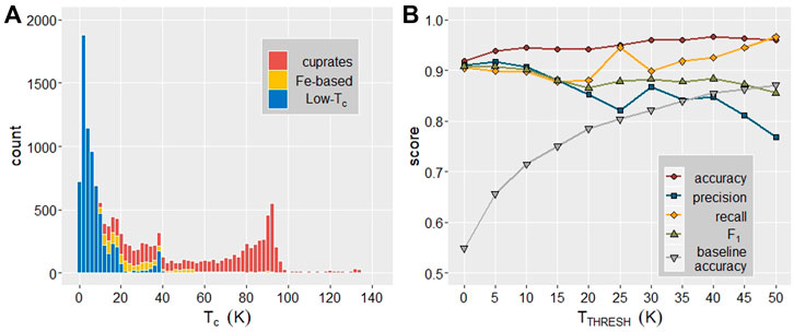
FIGURE 1. (A) Histogram of materials in the SuperCon dataset by T_C (bin width = 2 K). Blue, yellow, and red correspond to ‘Low-T_C’, iron-based, and cuprate superconductors, respectively. (B) Classification model performance as a function of a temperature threshold (T_THRESH) which partitions materials into two classes: above and below T_THRESH. Low-Tc is defined as superconductors with T_C < 40 K.

Convolutional Neural Networks

A variation on Xie and Grossmans’s Crystal Graph Convolutional Neural Network (CGCNN) is employed for classification and regression prediction of superconductivity, critical temperature, and other attributes. In the crystal-graph representation, edges of the graph represent connectivity between atoms and vertices of the graph represent atoms sites and their properties. In particular, the crystal-graph representation is recorded in three tensors which describe 1) the atom features, including atom species, 2) the distance of each atom site to its nearest neighbors 3) the identity of each atom site’s nearest neighbors. The atom feature tensor contains, for each atom site, a one-hot encoded vector which conveys, at minimum, the group and period number of the atom species at that site. The atom feature vector may also contain electronegativity, covalent radius, valence electrons, first ionization energy, electron affinity, block, and atomic volume of the site’s atom. In addition to the natural representation of crystal structures as graphs, we are further motivated by CGCNN’s performance in predicting attributes which are interconnected with superconductivity. Trained on dataset sizes of the order of ∼10,000, mean absolute error (MAE) for estimations of band gap energy, Fermi energy, and bulk moduli met or exceeded DFT-order accuracy for calculations of these properties (Xie and Grossman, 2018).

Convolutional neural networks are ideal for modeling superconductors and their properties due to their ability to model complex, nonlinear functions. These networks consist of several hidden layers, between input and output layers, which learn by experiencing data to represent a function. The hidden layers of a neural network are comprised of nodes which accept weighted input(s) from previous layers of the network. At each node, an activation function is applied to a linear combination of the weighted inputs; this value is sent to subsequent node(s) in subsequent layers of the network and introduces nonlinearity into the model. The neural network ‘learns’ during training by adjusting the weights connecting the nodes in the hidden layers through stochastic gradient descent. Specifically, at each iteration of training a randomly selected batch of data passes through the network and network performance is computed by evaluating the loss function on that batch of data. Then the gradient of the loss function is calculated via back-propagation and network weights are updated along the direction of steepest descent, the negative of the gradient. The magnitude of the weights’ update corresponds to the learning rate, another tunable parameter of neural networks (Goodfellow, et al., 2016). In this work, the classification and regression networks use negative log likelihood and mean absolute error loss functions, respectively. In convolutional neural networks, the hidden layers apply a convolution to the input volume which maps neighborhoods of the input volume into lower dimensions. Convolutional networks have been leveraged successfully to classify images, commonly referred to as ‘computer vision’ (Krizhevsky, et al., 2012). This construction is ideal for periodic structures because convolutions capture the local characteristics of the crystal structure.

For all CNNs described in this work, datasets are randomly split by 75% training, 10% validation, and 15% testing sets. The training process involves the CNN iteratively experiencing the entire training dataset, and updating (learning) through backpropagation, then experiencing the validation set to benchmark the model’s progress at that point in training. Each of these iterations is a single training ‘epoch’ and the number of training epochs used to train the CNN is a tunable model parameter. The validation set does not further train the network as network weights are not updated after experiencing the validation set. The testing set consists of samples which the network did not experience during training or validation. The trained network is applied to the testing set to estimate the network performance on out-of-sample populations of data; that is, data the network has never experienced. The training, validation, and testing datasets consist of crystal structure files for all compounds and their corresponding ground truth labels (e.g., experimentally measured critical temperature). In addition to the number of training epochs, tunable model parameters include the activation and loss functions, number of hidden layers, and number and type of atom features.

There are two main hazards regarding modeling with neural networks: overtraining and overfitting. Overtraining occurs when the network learns the gross features of the dataset but continues training and therefore ‘learns’ from noise in the dataset; an undesirable outcome as the network loses generalizability (Tetko, et al., 1995). Overtraining is avoided by halting training prior to network convergence; this is accomplished by examining network performance on a validation dataset after each epoch of training. After some number of epochs, validation loss (model error) will stop decreasing indicating the network’s performance on data it has not experienced is no longer improving. Overfitting occurs when the complexity within a network exceeds that required to model the function; in particular, predictive ability of neural networks may decline with increasing internal degrees of freedom (Andrea and Kalayeh, 1991). CGCNN already employs dropout, whereby elements of the input tensor are zeroed out with probability of 0.5; dropout is thought to reduce overreliance on particular features of training data thereby reducing overfitting (Hinton, et al., 2012). Additionally, benchmarking on number of hidden layers and atom features is used to determine the minimum complexity required for the CNN to model the dataset.

Representation of Off-Stoichiometric Compounds

Over two-thirds of the SuperCon database, ∼19,500 entries, have off-stoichiometric chemical compositions due to the varying substitutions and charge doping often required to elicit superconductivity; this is especially prevalent among the higher T_C materials. In general, the Materials Project does not contain all possible doping combinations or fractions; therefore, in the case an off-stoichiometric chemical composition does not correspond with an entry in the Materials Project, a ‘parent’ composition is determined heuristically and used to query the Materials Project instead. After a corresponding entry in the Materials Project is located, the structure file is corrected to reflect the true chemical composition. Further, for some entries, the SuperCon database contains experimentally determined lattice parameters which are used to correct atom coordinates and unit cell volume in the periodic crystal structure file. This practice increases the fidelity of the periodic structure file, especially in cases where a structure is substantially affected; for example, YBa₂Cu₃O_7-x, whose structure and superconductivity properties vary with oxygen fraction (Conder, 2001).

A probabilistic approach is employed to represent off-stoichiometric compositions to the neural networks. For an off-stoichiometric compound, the structure file generated will indicate multiple atom species at a single atom site, each with fractional occupancies that sum to the total coefficient of that site. In the data loading process, the crystal structure file is translated into the crystal-graph representation which requires the one-hot encoding of atom and neighbor features; this translation is complicated by the presence of multiple atom species at a single atom site. Specifically, multiple group and period numbers to describe multiple atom species cannot be represented in a one hot encoded vector. This is overcome by the following process: One-hot encoded vectors are instantiated to describe all doping species and parent species. For each atom site in the crystal, the possible dopant(s) and parent species at that site are identified. The one-hot encoded vectors for each species are scaled by the total fraction of the species at that atom site and then the vectors are added together. This results in a vector which contains the probability of each atom feature at each atom site.

Results

Classification Models

Several classification models are trained to classify whether a given compound is a superconductor and whether a given compound has a critical temperature greater than a threshold critical temperature (T_THRESH). All classification models are trained on a dataset of ∼22,000 compounds; ∼10,000 superconductors and ∼12,000 non-superconductors, including ∼200 non-superconducting copper oxide containing compounds. Non-superconducting compounds are considered to have zero T_C. The non-superconducting compounds are a diverse set of compounds collected from the Materials Project and cross-referenced with the SuperCon dataset to ensure no known superconductors are included. Although the compounds in the ‘non-superconductor’ category are ensured not to be known superconductors, there is a risk that undiscovered superconductors are inadvertently included in this class. The incidence of this is likely extremely small; a project which investigated over 1,000 expert-proposed superconductor candidates observed zero resistivity in just ∼3% of candidates (Hosono, et al., 2015).

Classification network performance is measured by precision, accuracy, recall, and F1 score. These performance metrics are defined by the following formulae:

$\text{accuracy}=\frac{\text{TP}+\text{TN}}{\text{TP}+\text{TN}+\text{FP}+\text{FN}}(1)$

$\text{precision}=\frac{\text{TP}}{\text{TP}+\text{FP}}(2)$

$\text{recall}=\frac{\text{TP}}{\text{TP}+\text{FN}}(3)$

${\text{F}}_1=2\times \frac{\text{precision}\times \text{recall}}{\text{precision }÷\text{recall}}(4)$

where TP, TN, FP, and FN represent number of true positive, true negative, false positive, and false negative results, respectively. In terms of the classification task of categorizing a material either as a superconductor or a non-superconductor these metrics are described by the following: A false positive is defined as the model classifying a compound as a superconductor when it is not actually one. Accuracy reflects the proportion of materials classified correctly. Precision is the proportion of model-classified superconductors which actually are superconductors and recall is the proportion of superconductors which the model identified. F1 score is the harmonic mean of precision and recall. Depending on the intended use of the trained neural network it may serve to optimize some parameters at the expense of the others; in training networks to search large materials databases a model with higher precision would be preferred because it may have fewer false positives.

Classification models are trained to determine whether a compound has critical temperature greater than a threshold temperature, T_THRESH. Performance measures for these models as a function of T_THRESH are shown in Figure 1B; baseline accuracy is the accuracy of a classification model that always selects the most populous category (i.e. always classifies compounds as having T_C < T_THRESH). For T_THRESH = 0K, baseline accuracy is equivalent to the proportion of compounds in the training dataset which are non-superconductors. In the range of T_THRESH from 0 to 15 K, all four performance metrics score ∼0.90 or higher with the best all-around model achieving accuracy of 95%. The T_THRESH = 20, 30 K models also perform well with all metrics >0.85 and may be the most useful to the goal of identifying high-T_C superconductors. Accuracy increases slightly as T_THRESH increases; this is an artifact of the proportion of compounds with T_C < T_THRESH increasing from 55% at 0K to 87% at 50 K, which allows the model to improve by simply classifying most compounds as having T_C below T_THRESH. Additionally, as T_THRESH increases, recall increases in line with precision decreasing. This trend is due to the increasing proportion of superconductors in the above-T_THRESH category which are cuprates. When nearly all superconductors in the above-T_THRESH category are cuprates, the classification model tends to classify most cuprate superconductors, even those with T_C far below T_THRESH, as having T_C > T_THRESH, resulting in reduced precision. Due to the varying T_THRESH, the training, testing, and validation datasets are necessarily all different and therefore there is some random variation of the performance metrics of these classification models.

Classification model performance as a function of training dataset size and several hyperparameters are benchmarked to determine optimal model hyperparameters. Performance as a function of these parameters can be found in Supplementary Figures S1, 2. SI Figure 1A shows model performance generally increasing as training dataset size increases. Model performance does not improve between training dataset sizes of 12,000 to 16,000 and even briefly declines. This implies additional data beyond 16,000 may not improve model performance substantially unless the additional data introduced new information to the networks. This might be achieved through higher quality datasets or the addition of new superconductor classes. For training dataset sizes below 8,500 it is difficult to quantify performance metrics and recognize model over-fitting as there are too few superconductors in the testing dataset and recall tends toward 0 (classifying all compounds as having T_C < T_THRESH ). SI Figure 1B shows model performance as a function of training batch size. Batch size is an important model parameter as it affects model convergence and generalizability. Larger batch sizes have been shown to reduce deep learning model’s ability to generalize and may tend to converge to non-optimal minima (Keskar, et al., 2017). Benchmarking the classification model performance indicates batch size between 25–50 results in best performance along all metrics. SI Figure 1C shows model performance with respect to the number of convolution layers. After four convolution layers, model performance does not improve by increasing the number of convolution layers. This indicates between 2–3 convolution layers is sufficiently complex to model the datasets. Model benchmarking of performance with respect to atom features is shown in SI Figure 2. Benchmarking finds, including block (s, p, d, f) in the atom feature vector results in the largest marginal increase in performance, second only to including all atom features. Interestingly, the atom feature valence electrons was ranked lowest in terms of performance improvement, indicating the valence orbital as opposed to the number of electrons is predictive. No combination of 3 or more atom features out-performs simply using all atom features. This is likely a result of neural networks being able to disregard (de-weight) information that is not important.

FIGURE 2

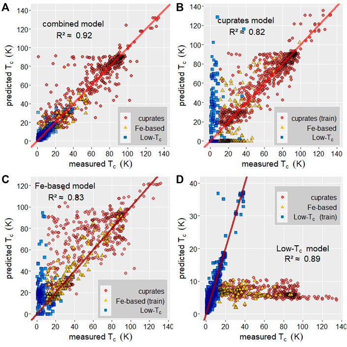
FIGURE 2. Regression model performance in predicting T_C, y = x shown as a solid, red line. (A) Predicted vs. measured T_C for a regression model trained on a combined dataset of cuprates, Fe-based, Low-T_C, and other compounds. R² ≈ 0.92. (B) Predicted vs. measured T_C for a regression model trained on cuprate superconductors only, model achieves R² ≈ 0.82 on cuprate-only test set. The cuprate-only model’s predicted T_C for Fe-based and Low-T_C compounds correlate poorly with measured values. (C) Predicted vs measured T_C for a regression model trained on Fe-based superconductors only, model achieves R² ≈ 0.83 on Fe-based-only test set. The Fe-based-only model’s predicted T_C for Low-T_C and cuprates correlates poorly with measured values. (D) Predicted vs. measured T_C for Low-T_C regression model trained on Low-T_C superconductors only, achieves R² ≈ 0.89 on Low-T_C only test set. The Low-T_C only model has no predictive ability on the Fe-based and cuprate test sets.

Classification models which can identify superconducting compounds with predictive accuracy, despite learning from only periodic crystal structure and chemical composition, are achieved and can be used to filter candidate compounds in materials databases. Since these models give no indication of critical temperature, CNNs are trained to accurately estimate critical temperature.

Regression Models

The second component of building a pipeline to search materials databases for new classes of high-T_C superconductors is a regression model which can estimate T_C with predictive accuracy. Performance metrics for regression models are R² value and mean absolute error (MAE). R² measures the test set correlation between measured T_C and model-predicted T_C and MAE is calculated by the formula:

$\text{MAE}=\frac{1}{N}{\displaystyle \sum }_1^N|T_{meas}-T_{pred}|(5)$

where N is the size of the test set, and T_meas and T_pred correspond to measured T_C and model-predicted T_C, respectively.

Regression models are trained on a dataset of the periodic crystal structure file and experimentally measured T_C for over 10,000 superconductors from the SuperCon database. No non-superconducting materials are included in these sets. Figure 2A shows a regression model trained on all superconducting materials which achieves R² ≈ 0.92 and MAE = 5.6. Figures 2B–D show model predicted T_C vs. measured T_C for regression models trained on only copper-oxide containing superconductors with T_C > 10K, Fe-based superconductors with T_C > 10 K, and superconductors with T_C < 40 K (low-T_C) which fall into neither of the other two categories. Although visually, in Figure 2D T_C = 20 K is a more natural cutoff for the Low-T_C category, the compounds in the low-T_C class with T_C > 20 K include the phonon-mediated diboride superconductors, Mg_1-xM_xB₂ (M = Al, C, Co, Fe, Li, Mn, Ni, Si, Zn) (Buzea and Yamashita, 2001) and Ba_1-xK_xBiO₃ (Yin, Kutepov, and Kotliar, 2013). Despite the unusually high T_C’s these superconductors are adequately modeled by the Low-T_C trained network, and indicates that our networks are picking them out as being similar in mechanism as other low-T_c materials. The cuprate, Fe-based, and low-T_C models achieve R² ≈ 0.82 and MAE = 8.0 K, R² ≈ 0.83 and MAE = 6.4 K, and R² ≈ 0.89 and MAE = 1.6 K, respectively. Note that the range of T_C for the Low-T_C model is 0–40 K while the range of possible T_C for the cuprate and Fe-based models is 10–140 K; this difference accounts for the much lower MAE for the low-T_C model.

The combined model’s R² value by material class is 0.82, 0.73, and 0.81 for the cuprate, Fe-based, and Low-T_C classes, respectively. This indicates that individual classes are better modeled by the individual-class models than by the combined model. Model bias, represented by the distribution of relative errors, for each of the four regression models is shown in SI Figure 3. Each of the models is slightly biased toward underestimation of T_C with the cuprate-only model being the least biased. Figures 1B–D also indicate how well each of the individual models can predict T_C for the other two classes by plotting the individual models’ predicted T_C for a static test set. In general, the individual class models have little to no predictive power for the other two classes. The cuprate model significantly overestimates the Low-T_C superconductors and a large portion of Fe-based superconductors are estimated to have T_C near 0 K. Similarly, the Fe-based model overestimates the Low-T_C superconductors with large variations in its predictions of T_C for cuprates. The Low-T_C model demonstrates no predictive power for the other two classes; it estimates most cuprate and Fe-based superconductors to have T_C < 10 K.

FIGURE 3

FIGURE 3. Atom feature importance in terms of regression model performance, as measured by R² and MAE calculated on the test set, for individual-class models. The x-axis indicates which atom feature, in addition to group and period, is included in the model. In each of the subplots, the x-axis is in order of increasingly good performance. The right-most x-axis category, ‘all features’, is the category with best performance for all three models. (A) Cuprate model performance vs atom features. (B) Fe-based model performance vs atom features. (C) Low-T_C model performance vs. atom features.

Unlike decision-tree based models, where features can be ranked by their marginal improvement to the model performance, it is not clear how to determine which features the neural networks relied upon most. However, the relative importance of the atom features may be gleaned by benchmarking model performance on different atom feature vectors. Performance is benchmarked for each of the individual-class models in an attempt to understand the different mechanisms at play in each class. Figure 3 contains performance of the cuprate, Fe-based and Low-T_C models for various atom feature vectors. The x-axis indicates which atom feature, in addition to group and period, is included in the crystal-graph used to train the models. For each of the individual-class models, those trained using only group and period still perform well and the best performance in each class was the model trained using all nine atom features. Additionally, no combination of three or more features performs better than using all nine atom features; this is likely due to the CNN’s ability to disregard unhelpful features through de-weighting.

Figures 3A–C indicate the single atom feature corresponding to best model performance in each of the cuprate, Fe-based, and Low-T_C models. The Low-T_C model best single feature was covalent radius, although models trained with this feature only barely outperformed the two next-best features: valence electrons and first ionization energy. The slightly increased relative importance of covalent radius and valence electrons reflect long standing experimental results. Among elemental, alloy and some other compound superconducting materials, T_C is proportional to atomic volume by the relation T_C ∼ V^x, where x = 4,5 (Matthias, 1955), and T_C is indirectly proportional to ionic mass: T_C ∼ 1/ $\sqrt{m_I}$ (Reynolds, et al., 1951). In second place, valence electrons reflect the finding that 2 to 8 valence electrons per atom are generally required for superconductivity in this class with T_C of non-transition metals increasing for increasing valence electrons per atom and T_C peaking at 3, 5, and 7 valence electrons per atom in transition metals (Matthias, 1955). In the Fe-based model, the 6 best single atom features perform similarly; therefore, for the Low-T_C and Fe-based models it is best to include group and period only in the atom feature vector for increased generalizability.

The cuprate regression model is an exception; the single best feature, first ionization energy, performs substantially better than models trained using other atom features. Figure 4 examines the relationship between the sum of first ionization energies of the cations and T_C. The maximum T_C observed increases with increasing ionization energy; variation of T_C within the same ionization energy is due to other factors including oxygen reduction. It has been determined previously for the Buckminster fullerides, A₃C₆₀, that decreases in the sum of ionization energies of the alkali atoms corresponds with increasing T_C (Hetfleisch, et al., 2015), so in the cuprates trends in ionization energy have the opposite effect. This likely reflects that the fullerides are electron-doped in nature, whereas the cuprates are almost exclusively hole doped, though it may also reflect different underlying mechanisms. We note that for both the iron and cuprate superconductor families, first ionization energy and electronegativity are in the best performing individual features. This is in agreement with chemical intuition, which has identified metal ligand covalency as a key ingredient in high-T_C superconductors.

FIGURE 4

FIGURE 4. T_C vs. sum of first ionization energies of cations in cuprate superconductors. Maximum attainable T_C increases with sum of ionization energy of the cations. Red, dashed line indicates upper limit on T_C vs. ionization energy.

Benchmarking of regression model parameters including training dataset size, epochs of training, and the number of convolution layers is carried out to optimize model performance. Figure 5A shows the combined regression model performance as a function training dataset size to increase from sizes of 0–4000 and then plateau between 4000 and 8000. Similar to the classification model, this indicates simply training with more data may not increase predictive accuracy. Figure 5B similarly indicates a point of diminishing returns with respect to the number of training epochs; model training is halted prior to 120 epochs to reduce the potential loss of generalizability from overtraining. Figure 5C finds the optimal number of network convolution layers to be five, an increase over the optimal number for the classification networks indicating the increased complexity of modeling the continuous variable T_C over a binary classification problem (larger number of layers will eventually lead to overfitting/memorization).

The combined T_C regression model trains on a dataset of superconductors only. An interesting finding, therefore, is that when posing a test set of 2500 superconductors and non-superconductors, for which T_C is set to 0, the regression model distinguished between the two sets extremely well. This is surprising because all of the materials the regression network experiences in training have T_C > 0 K. In particular, the combined regression model classifies whether a compound has T_C > 30 K, with greater accuracy than the classification model described previously. Figure 6 details the classification ability of the combined regression model as a function of T_THRESH.

FIGURE 5

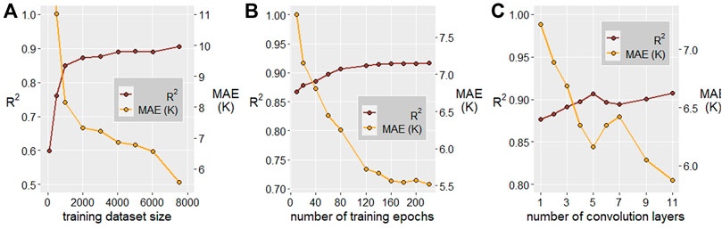
FIGURE 5. Combined regression model performance, measured by R² and MAE, as a function of various model parameters. (A) Performance vs. training dataset size. (B) Performance vs. number of training epochs. (C) Performance vs. number of convolution layers. Five layers optimizes both performance metrics.

FIGURE 6

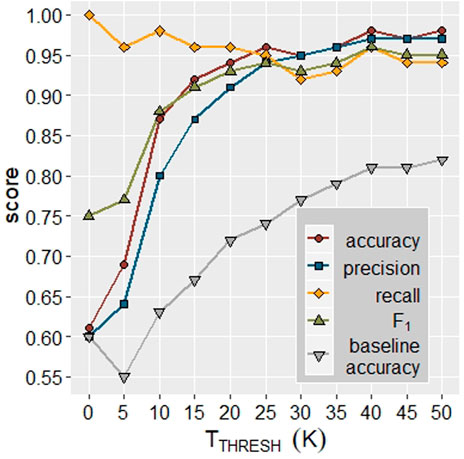
FIGURE 6. Performance of all-class T_C regression model when tested on a dataset of ∼2500 superconductors and non-superconductors. Non-superconductors are assumed T_C = 0. Baseline accuracy is the calculated accuracy for a model which always recommends the classification of the most populous category.

As previously mentioned, each superconductor from the SuperCon database is associated with 173 material-specific attributes and attributes for which there are sufficient data are used to train a regression network. The logarithm of Debye temperature and coefficient of electronic specific heat, and Néel temperature are modeled by CNNs with some success: R² is roughly 0.68 for these models despite having fewer than 800 and as little as 400 materials in the training dataset. These models indicate a wider use of CNNs beyond predicting only T_C.

Search for New Superconductors in the Materials Project

Ultimately, the purpose of models which accurately classify superconductors and predict material-specific properties is to select candidate materials with desirable properties, in this case high T_C. As a proof of concept, we use the classification and regression models, combined into a single pipeline, to search for candidate high temperature superconductors among the 130,000 unique compositions in the Materials Project. Around half of all candidates with predicted T_C >25 K were copper-oxide containing or Fe-based; as the training dataset consisted of largely these two classes, in the T_C >25 K range, it is not surprising that the networks mostly found candidates within these categories. The overall positivity rate is 3.7% indicating the pipeline is not as biased toward a positive classification as might be expected for a model trained by a dataset of 40% superconductors and 60% non-superconductors. Just over 2% (∼2800) compounds in the Materials Project database are predicted to have T_C > 25 K and are not copper-oxide containing or Fe-based; 85% of this group contains oxygen, not surprising given the distribution of the training data. Figure 7 shows the distribution of candidate materials, with a close view of potential new classes of high temperature superconductors.

FIGURE 7

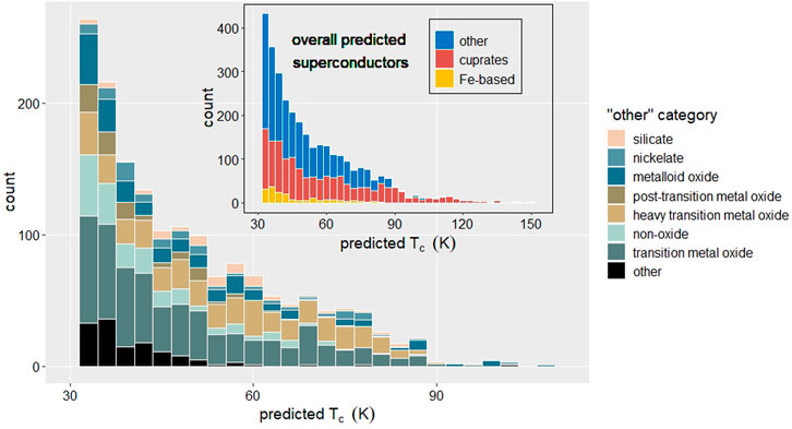
FIGURE 7. Distribution of model-predicted candidate superconductors. Inset figure describes overall distribution of candidates with a closer view of potential new classes of high temperature superconductors.

We examine the pipeline’s candidates with predicted T_C >25 K and which do not belong to established superconductor classes and propose several high-T_C candidates in Table 1. The most numerous group of candidates are the transition metal oxides containing Ni, Pd, Ru, and Ag. This should motivate advances in synthesis to higher oxygen partial pressures necessary to stabilize the high oxidation states of Ru, Pd, etc, found in these predicted materials. Interestingly, heavier transition metal oxides containing Ta, Re, Os, and Ir also make up a large fraction of these candidates. Many of these candidates appear analogous to cuprate and pnictide superconductors; crystal structure and simple chemical patterns such as valence electrons, charge balancing, and stoichiometry were likely identified by the neural networks. On this basis, it is natural to ask why superconductivity has not, to date, been observed in these materials; one distinct possibility is that it has not (yet) been possible to prepare sufficient quality and electron-count controlled versions. This is supported by the nickelate candidates: ANiO₂ (A = Mg, Ca, Ba), which relate to the recent observation of zero resistivity between 9 and 15 K in the rare-earth infinite-layer nickelate, Nd_0.8Sr_0.2NiO₂ (Li, et al., 2019), even though the materials themselves have been known for decades.

TABLE 1

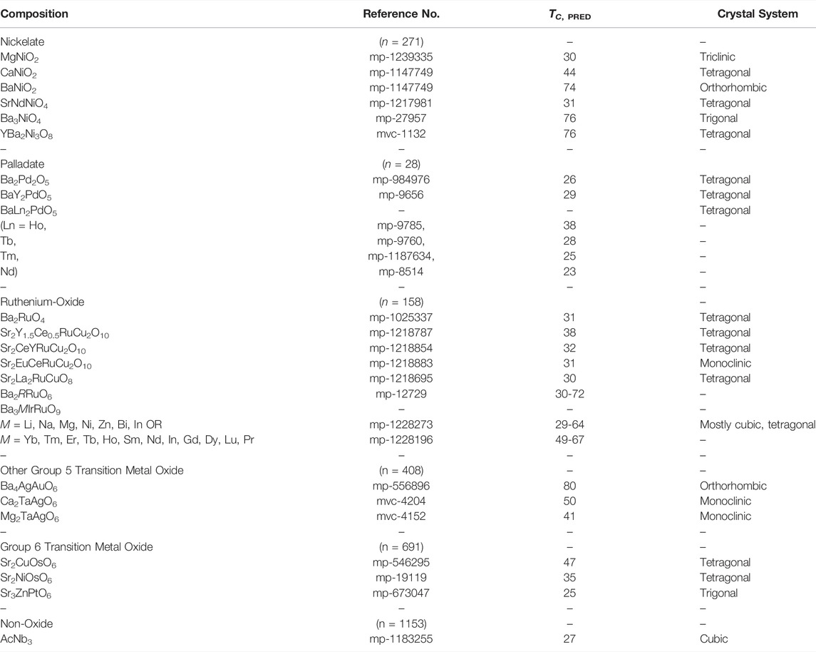
TABLE 1. Superconductor candidates classified by the model with Materials Project reference number, model-predicted T_C, and crystal system. Number of model proposed candidates with T_C >25 K in parenthesis.

Ruthenium oxides are the next most numerous group; in addition to candidates with cuprate analogs, the triple perovskites Ba₃MIrRuO₉ (M = Li, Na, Mg, Ni, Zn, Bi, In) and Sr₂Y_1+xCe_1-xRuCu₂O₁₀ (x = 0, 0.5), with alternating copper oxide and ruthenium oxide layers are interesting candidates. Superconductivity in the heavier transition metal oxides is not unprecedented although it has not yet been observed at the high model-predicted temperatures herein. The layered silver oxide, Ag₅Pb₂O₆, superconducts at very low temperatures (Yonezawa and Maeno, 2005) and in the pyrochlore oxides RbOs₂O₆ and Cd₂Re₂O₇ at 6.3 and 1 K, respectively (Hanawa, et al., 2001; Yonezawa, et al., 2004). Also surprising is the prediction of intermetallic oxides and metalloid candidates including silicon oxide and germanates. While it is unlikely the stoichiometric compositions are superconducting, it is possible various experimental methods including substrates, pressure, and charge doping can bring about or enhance a phase transition in these candidate classes if they can be successfully electron doped (a formidable chemical challenge itself) (Chamorro and McQueen, 2018).

Discussion

Convolutional neural networks are leveraged to model superconducting critical temperature and screen the Materials Project for new families of high T_C candidate materials. Crystal structures are represented to the CNNs as undirected graphs and no explicit chemical attributes beyond composition are required to achieve good performance. The best regression model can predict critical temperature with an average absolute error of 5.6 K, with slight bias toward underestimation. This regression model also accurately classifies whether a crystal has T_C above a threshold value with F1 >0.94 for T_THRESH = 25 K; both superconductors and non-superconductors are accurately classified by this model despite it training on a dataset of superconductors only. Combining classification and regression models into a pipeline and searching the Materials Project crystal structure database yields 2800 superconductor candidates with predicted T_C >25 which are not copper-oxide containing or Fe-based. The significant variety in predicted candidates combined with the prediction of cuprate and pnictide analogs is indicative of the generalizability of these models. These models appear to be especially useful for uncovering high-T_C superconductivity in perovskite structures as small changes in stoichiometry or reduction can generate significant changes in T_C and other properties. While it is unknown whether any of the candidate materials are superconducting, similar models may be trained on individual classes of superconductors to generate phase diagrams and determine optimal substitution elements and ratios to optimize T_C or other attributes in these materials.

Although accounting for crystal structure is a step forward, future iterations of these models would be improved by increasing the complexity of the crystal-graph representation to account for various substrates, topologies, and pressure often used to bring about superconductivity or enhance T_C. As the current record for high-T_C superconductivity is thought to have been achieved with hydrogen rich mixtures (e.g. H₃S, YH₁₀) under extreme pressure, not accounting for pressure specifically may limit future models (Drozdov, et al., 2019). These attributes could be incorporated into the models used herein implicitly by adjusting compounds’ structure and stoichiometry to reflect the behavior of the structure under high pressure, for example, or to reflect the presence of a substrate. Alternatively, these parameters could be represented explicitly as a binary (pressure, no pressure), categorical, or continuous variable. The crystal-graph is ultimately three tensors of numbers and so may be made arbitrarily complex to account for these important experimental variables. Either approach requires a richer dataset than what is currently available, although efforts toward this goal are in motion.

Although the crystal-graph representation is powerful and flexible there are drawbacks to artificial neural networks more generally. Data loading from crystal structure files and model training require significant computational time and memory. Despite this, the pre-trained models themselves can screen large databases quickly with the majority of time and memory being used to load the crystal structure data. Another drawback of artificial neural networks is interpretability; it is not clear what features of the superconductors the models picked up on to predict T_C or classify a material as a superconductor or not. Due to this, neural networks may not be the best choice of model if the goal is to glean physical insights. This is especially difficult, in light of the models performing similarly whether explicit atom features (valence electrons, block, etc.) are included in the crystal-graph representation or not. Methods to overcome this are in development; image classification tasks can be interpreted by scores on each pixel on a predicted image with the score indicating how much that pixel contributed to the network’s decision (Lundber and Lee, 2017). A similar scoring may be implemented for the crystal-graph and visualized to determine which aspects of the graph were most important in the model’s prediction.

Data Availability Statement

The datasets presented in this study can be found in online repositories. The names of the repository/repositories can be found in the Supplementary Material.

Author Contributions

The authors confirm their contributions to the paper as the following: study conception and design, candidate materials analysis, manuscript revision: MRQ and TMM; dataset acquisition and data engineering, network and pipeline design and coding, data collection and analysis: MRQ. All authors contributed to the manuscript.

Funding

The Rockfish cluster is supported by the National Science Foundation grant number OAC 1920103.

Conflict of Interest

The authors declare that the research was conducted in the absence of any commercial or financial relationships that could be construed as a potential conflict of interest.

Publisher’s Note

All claims expressed in this article are solely those of the authors and do not necessarily represent those of their affiliated organizations, or those of the publisher, the editors and the reviewers. Any product that may be evaluated in this article, or claim that may be made by its manufacturer, is not guaranteed or endorsed by the publisher.

Acknowledgments

MQ acknowledges support by the Johns Hopkins University, Krieger School of Arts and Sciences, Dean’s Undergraduate Research Award. TM acknowledges support of the David and Lucile Packard Foundation. Calculations were performed using computational resources of the Maryland Advanced Research Computing Center and the Advanced Research Computing at Hopkins (ARCH) Rockfish cluster.

Supplementary Material

The Supplementary Material for this article can be found online at: https://www.frontiersin.org/articles/10.3389/femat.2022.893797/full#supplementary-material

References

Andrea, T. A., and Kalayeh, H. (1991). Applications of Neural Networks in Quantitative Structure-Activity Relationships of Dihydrofolate Reductase Inhibitors. J. Med. Chem. 34, 2824–2836. doi:10.1021/jm00113a022

PubMed Abstract | CrossRef Full Text | Google Scholar

Bednorz, J. G., and Muller, K. A. (1986). Possible highT C Superconductivity in the Ba?La?Cu?O System. Z. Physik B - Condensed Matter 64, 189–193. doi:10.1007/bf01303701

CrossRef Full Text | Google Scholar

Buzea, C., and Yamashita, T. (2001). Review of the Superconducting Properties of MgB2. Supercond. Sci. Technol. 14, R115–R146. doi:10.1088/0953-2048/14/11/201

CrossRef Full Text | Google Scholar

Chamorro, J. R., and McQueen, T. M. (2018). Progress toward Solid State Synthesis by Design. Acc. Chem. Res. 51, 2918–2925. doi:10.1021/acs.accounts.8b00382

PubMed Abstract | CrossRef Full Text | Google Scholar

Conder, K. (2001). Oxygen Diffusion in the Superconductors of the YBaCuO Family: Isotope Exchange Measurements and Models. Mater. Sci. Eng. R: Rep. 32, 41–102. Issues 2–3ISSN 0927-796X. doi:10.1016/s0927-796x(00)00030-9

CrossRef Full Text | Google Scholar

Drozdov, A. P., Kong, P. P., Minkov, V. S., Besedin, S. P., Kuzovnikov, M. A., Mozaffari, S., et al. (2019). Superconductivity at 250 K in Lanthanum Hydride under High Pressures. Nature 569, 528–531. doi:10.1038/s41586-019-1201-8

PubMed Abstract | CrossRef Full Text | Google Scholar

Goodfellow, I., Bengio, Y., and Courville, A. (2016). Deep Learning. Cambridge, Massachusetts: The MIT Press.

Google Scholar

Hetfleisch, F., Stepper, M., Roeser, H.-P., Bohr, A., Lopez, J. S., Mashmool, M., et al. (2015). A Correlation between Ionization Energies and Critical Temperatures in Superconducting A3C60 Fullerides. Physica C: Superconductivity its Appl. 513, 1–3. ISSN 0921-4534. doi:10.1016/j.physc.2015.02.048

CrossRef Full Text | Google Scholar

Hinton, G. E., Srivastava, N., Krizhevsky, A., Sutskever, I., and Salakhutdinov, R. (2012). Improving Neural Networks by Preventing Co-adaptation of Feature Detectors. 0580. Available at: https://arxiv.org/abs/1207.0580.

Google Scholar

Hosono, H., Tanabe, K., Takayama-Muromachi, E., Kageyama, H., Yamanaka, S., Kumakura, H., et al. (2015). Exploration of New Superconductors and Functional Materials, and Fabrication of Superconducting tapes and Wires of Iron Pnictides. Sci. Technol. Adv. Mater. 16, 033503. doi:10.1088/1468-6996/16/3/033503

PubMed Abstract | CrossRef Full Text | Google Scholar

Jain, A., Ong, S. P., Hautier, G., Chen, W., Richards, W. D., Dacek, S., et al. (2013). Commentary: The Materials Project: A Materials Genome Approach to Accelerating Materials Innovation. APL Mater. 1 (1), 011002. doi:10.1063/1.4812323

CrossRef Full Text | Google Scholar

Keskar, N., Mudigere, D., Nocedal, J., and Smelyanskiy, M. (2017). “On Large-Batch Training for Deep Learning: Generalization Gap and Sharp Minima,” in Conference International Conference on Learning Representations (ICLR), Toulon, France. Available at: https://arxiv.org/pdf/1609.04836.pdf.

Google Scholar

Konno, T., Kurokawa, H., and Nabeshima, F. (2021). Deep Learning Model for Finding New Superconductors. Phy. Rev. B 03, 014509. doi:10.1103/physrevb.103.014509

CrossRef Full Text | Google Scholar

Krizhevsky, A., Sutskever, I., and Hinton, G. E. (2012). “ImageNet Classification with Deep Convolutional Neural Networks,” in Advances in Neural Information Processing Systems 25, (NIPS 2012), Lake Tahoe, NV. Available at: https://proceedings.neurips.cc/paper/2012/file/c399862d3b9d6b76c8436e924a68c45b-Paper.pdf.

Google Scholar

Li, D., Lee, K., Wang, B. Y., Osada, M., Crossley, S., Lee, H. R., et al. (2019). Superconductivity in an Infinite-Layer Nickelate. Nature 572, 624–627. doi:10.1038/s41586-019-1496-5

PubMed Abstract | CrossRef Full Text | Google Scholar

Lundberg, S. M., and Lee, S. (2017). “A Unified Approach to Interpreting Model Predictions,” in Advances in Neural Information Processing Systems 30 (NIPS 2017), Long Beach, CA. NIPS. Available at: https://arxiv.org/abs/1705.07874.

Google Scholar

Marques, M. A. L., Lüders, M., and Lathiotakis, N. N. (2005). Ab Initio theory of Superconductivity. II. Application to Elemental Metals. Phys. Rev. B 72, 024546. doi:10.1103/physrevb.72.024546

CrossRef Full Text | Google Scholar

Matthias, B. T. (1955). Empirical Relation between Superconductivity and the Number of Valence Electrons Per Atom. Phys. Rev. 97, 74–76. doi:10.1103/physrev.97.74

CrossRef Full Text | Google Scholar

National Institute of Materials Science (2011). Materials Information Station, SuperCon. Available at: http://supercon.nims.go.jp/index en.html (Accessed Aug 15, 2021).

Google Scholar

Reynolds, C. A., Serin, B., and Nesbitt, L. B. (1951). The Isotope Effect in Superconductivity. Mercury. Phys. Rev. 84, 691. doi:10.1103/PhysRev.84.691

CrossRef Full Text | Google Scholar

Sanna, A., Pellegrini, C., and Gross, E. K. U. (2020). Combining Eliashberg Theory with Density Functional Theory for the Accurate Prediction of Superconducting Transition Temperatures and Gap Functions. Phys. Rev. Lett. 125, 057001. doi:10.1103/PhysRevLett.125.057001

PubMed Abstract | CrossRef Full Text | Google Scholar

Stanev, V., Oses, C., Kusne, A. G., Rodriguez, E., Paglione, J., Curtarolo, S., et al. (2018). Machine Learning Modeling of Superconducting Critical Temperature. Npj Comput. Mater. 4, 29. doi:10.1038/s41524-018-0085-8

CrossRef Full Text | Google Scholar

Tetko, I. V., Livingstone, D. J., and Luik, A. I. (1995). Neural Network Studies. 1. Comparison of Overfitting and Overtraining. J. Chem. Inf. Comput. Sci. 35 (5), 826–833. doi:10.1021/ci00027a006

CrossRef Full Text | Google Scholar

Villars, P., and Phillips, J. (1988). Quantum Structural Diagrams and High-T_{c} Superconductivity. Phys. Rev. B 37, 2345–2348. doi:10.1103/physrevb.37.2345

PubMed Abstract | CrossRef Full Text | Google Scholar

Ward, L., Agrawal, A., Agrawal, A., Choudhary, A., and Wolverton, C. (2016). A General-Purpose Machine Learning Framework for Predicting Properties of Inorganic Materials. Npj Comput. Mater. 2, 16028. doi:10.1038/npjcompumats.2016.28

CrossRef Full Text | Google Scholar

Wu, M. K., Ashburn, J. R., Torng, C. J., Hor, P. H., Meng, R. L., Gao, L., et al. (1987). Superconductivity at 93 K in a New Mixed-phase Y-Ba-Cu-O Compound System at Ambient Pressure. Phys. Rev. Lett. 58, 908–910. doi:10.1103/physrevlett.58.908

PubMed Abstract | CrossRef Full Text | Google Scholar

Xie, T., and Grossman, J. C. (2018). Crystal Graph Convolutional Neural Networks for an Accurate and Interpretable Prediction of Material Properties. Phys. Rev. Lett. 120, 145301. doi:10.1103/physrevlett.120.145301

PubMed Abstract | CrossRef Full Text | Google Scholar

Yamashita, R., Nishio, M., Do, R. K. G., and Togashi, K. (2018). Convolutional Neural Networks: an Overview and Application in Radiology. Insights Imaging 9, 611–629. doi:10.1007/s13244-018-0639-9

PubMed Abstract | CrossRef Full Text | Google Scholar

Yin, Z. P., Kutepov, A., and Kotliar, G. (2013). Correlation-Enhanced Electron-Phonon Coupling Applications of GW and Screened Hybrid Functional to Bismuthates, Chloronitrides, and Other High-Tc Superconductors. Phys. Rev. X 3, 021011.

CrossRef Full Text | Google Scholar

Yonezawa, S., and Maeno, Y. (2005). Type-I Superconductivity of the Layered Silver oxideAg5Pb2O6. Phys. Rev. B 72, 180504. doi:10.1103/physrevb.72.180504

CrossRef Full Text | Google Scholar

Yonezawa, S., Muraoka, Y., Matsushita, Y., and Hiroi, Z. (2004). New Pyrochlore Oxide Superconductor RbOs2O6. J. Phy. Soc. Jpn. 73, 819–821.

CrossRef Full Text | Google Scholar