 Xianglei Ye
 Zhenya Ji
 Jinxing Xu
 Xiaofeng Liu
95% of researchers rate our articles as excellent or good
Learn more about the work of our research integrity team to safeguard the quality of each article we publish.
Find out more
ORIGINAL RESEARCH article
Front. Electron. , 23 February 2023
Sec. Industrial Electronics
Volume 4 - 2023 | https://doi.org/10.3389/felec.2023.1110039
This article is part of the Research Topic Re-electrification Technology and Application of the Energy Consumption Terminal View all 4 articles
The integrated energy system is an effective way to achieve carbon neutrality. To further exploit the carbon reduction potentials of IESs, an optimal dispatch strategy that considers integrated demand response and stepped carbon trading is proposed. First, an integrated demand response (IDR) pricing approach is proposed based on the characteristics of different load types. Classify multi-energy loads into curtailable and substitutable loads, and incentivize both loads through a price elasticity matrix and low-price energy in the same period. Then, to better incentivize IESs to reduce carbon emissions, a stepped pricing mechanism was introduced in the carbon price. Finally, an optimal dispatch model is developed with an objective function that minimizes the sum of energy purchase cost, carbon trading cost, and operation and maintenance (O&M) cost. Considering the high-dimensional and non-linear characteristics of the model, an improved differential evolution (DE) algorithm is introduced in this paper. In addition, this paper also analyzes the effects of the stepped carbon trading parameters on the optimal dispatching results of the system in terms of carbon trading base price, carbon emission interval length, and carbon price growth rate. Compared to the case of adopting a single IDR model or a single stepped carbon trading, carbon emissions from the IESs decreased by 6.28% and 3.24%, respectively, while total operating costs decreased by 1.24% and 0.92%, The results show that the model proposed in this paper has good environmental and economic benefits, and the reasonable setting of stepped carbon trading parameters can effectively promote the low-carbon development of IESs.
Nowadays, the greenhouse effect is serious and energy consumption lacks sustainability due to the increase of a large amounts of fossil energy consumption. How to promote the transformation of energy structure and make the system achieve low-carbon economic operation is an urgent issue to be solved. The integrated energy system (IES) can reduce operating costs by coupling multiple independent energy systems such as electricity, gas, and heat to achieve complementary and synergistic multi-energy sources. However, the allocation of various energy sources in IESs and the dispatching strategies of different devices directly affect the economy and the efficiency of energy use. Therefore, it is important to investigate how to make the operation of IESs meet the needs of the customer side while achieving the efficient goal of a low carbon economy.
Due to the popularity of demand-side management, demand response (DR) techniques are widely used in traditional power systems (Luo et al., 2019). In the study of lhsan et al. (2019), DR was introduced to encourage customers to optimize their electricity consumption behavior through flexible pricing policies that bring benefits and improve operational efficiency on the supply side. Lynch et al. (2019) introduced DR to encourage customers to respond to system dispatch by implementing a differentiated tariff policy, which alleviated the shortage of electricity in the public grid. However, the above literature only considers DR in the traditional electricity system, which cannot fully utilize the interactive capability of demand-side resources. Therefore, on the basis of traditional power DE, Integrated Demand Response (IDR) (Wang et al., 2017) came into being. Among them, Wang et al. (2020a) proposed an IES bi-objective operation optimization model considering the IDR mechanism for electric and heat loads. In literature (Liu et al., 2019), three levels of multi-energy day market structure and operation mechanism that allows simultaneous trading of electricity, heat, and natural gas are proposed based on the optimal trading strategy modeling of IDR. Li et al. (2021) introduced horizontal complementarity and vertical time-shifting strategies for electricity, gas, and heat to establish a stochastic robust optimal operating model based on IDR, which effectively reduces operating costs. However, most of the above IDR models model the demand response in terms of energy types, and although the differences in the characteristics of multiple energy sources are considered, the important role of different DR types of a single energy source and the mutual substitution of multiple energy sources is ignored. Therefore, in this paper, IDR is divided into the curtailable load (CL), shiftable load (SL), and replaceable load (RL). Demand response modeling based on IDR types.
The above studies on IESs optimal dispatching have been done from an economic perspective (Gu et al., 2017; Wang B et al., 2022). The impact of carbon emission on IESs dispatch is not considered. To improve this point, Cheng et al. (2019) studied the low carbon operation of IES by coordinating the transmission-level and distribution-level via the energy-carbon integrated prices. Xiong et al. (2022) considered the low-carbon nature of the system and established a low-carbon economic operation model of the power system. Zhang et al. (2021) also considered carbon emissions and discussed the impact of carbon emissions on wind power consumption. With the proposal of a carbon trading market (Cao et al., 2022; Wang et al., 2020b), carbon emission allowances have also evolved into a carbon trading mechanism. In the existing literature, most of the traditional carbon trading mechanism models currently applied are fixed-value models (Li et al., 2019a; Wang et al., 2020c; Wang et al., 2020d; Hu et al., 2021). Based on this point. In the study by Wang B et al. (2022), a step carbon trading mechanism was proposed to address the shortcomings of the traditional carbon trading mechanism. In addition, Guo et al. (2022) introduced the stepped carbon trading mechanism into the IESs optimal dispatching model and established a multi-objective optimal dispatching model containing economic and environmental objectives. However, there is little literature on the application of the ladder carbon trading mechanism that also considers IDR, so a comprehensive consideration of the ladder carbon trading mechanism and IDR is the focus of this paper.
In the problem of solving the model for the stepped carbon trading mechanism, Ma et al. (2022) adopted the segmented linear method to deal with the quadratic term part of the objective function, but the treatment of the objective function is mostly approximate calculation, which lacks accuracy and comprehensive consideration. In order to improve the above problems, Wu et al. (2022) used the particle swarm algorithm to solve the system optimization model, but the particle swarm algorithm was difficult to set the appropriate inertia weights, and it was easy to make the algorithm fall into local optimal solutions. The traditional DE algorithm (Mi, 2022) is also used to solve the complex objective function with the risk of premature aging.
Based on the above research, this paper proposes an optimal dispatching strategy for IESs considering IDR strategy and stepped carbon trading. An improved DE algorithm is used to solve the model developed in the paper. Based on the traditional model, the following additions are made.
1) IDR is considered in the multi-energy load section of IESs. The multi-energy loads are categorized and modeled by various DR types. A proposed IDR model with CL, SL, and RL is also included.
2) In this paper, a stepped carbon trading mechanism is also considered in the optimal dispatch of the IESs, and a stepped carbon price is set with rewards and penalties. With the minimum value of energy purchase cost, O&M cost, and carbon trading cost of the system as the objective function, a low-carbon economic operation model of the IESs is established.
3) Because the model constructed in this paper is a highly non-linear programming problem. In this study, an improved DE algorithm is used to solve the dispatching model, The algorithm is improved in two aspects: the adaptive operator and the variational strategy, which improves the convergence and efficiency of the procedure.
The energy supply side mainly includes wind turbines (WT), photovoltaic (PV), upper electrical grid, and upper gas grid. In the energy trading section, IES purchases electricity and natural gas from the upper power grid and the upper gas grid. Among the multi-energy coupling devices, the combined heat and power (CHP) system in the IES mainly consists of a gas turbine (GT), a waste heat boiler (WHB), and a low-temperature waste heat generator based on the organic Rankine cycle (ORC). The operation mode is thermal-electrolytic coupling, which can adapt to different operating conditions of the system and meet the requirements of system stability. In addition, the system also includes a gas boiler (GB) and heat pump (HP), which help to consume wind power and take up part of the heat load at the same time, realizing the two-way flow of electricity and heat energy. Electric energy storage (ES), heat energy storage (HS), and gas energy storage (GS) are the energy storage devices in the IES. The structure of the IES and the IDR in this paper is shown in Figure 1.
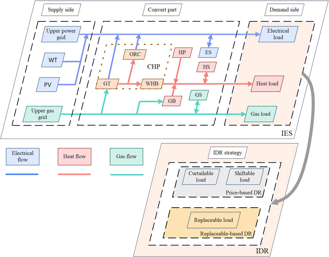
FIGURE 1. The structure of the IES and the IDR.
The IDR model constructed in this paper mainly includes price-based DR and replaceable-based DR, which realize the transfer of multiple loads in horizontal time and mutual substitution in vertical time, respectively. The IDR model is developed below according to the types of multi-demand responses.
Different types of loads differ in their sensitivity to the same electricity price signal, and the price-based DR electrical loads are divided into the CL and SL, and these two types of loads are modeled separately below.
For curtailable electric load, it means that the customer can reasonably curtail part of his electric load without affecting his satisfaction with energy use according to the price information. The DR characteristics are described by the price-demand elasticity matrix. The element in the tth row and jth column of the elasticity matrix
where,
According to the power elasticity matrix established by the above equation, the amount of change in CL at time t after DR is defined as:
where,
SL refers to the flexibility of customers to adjust their load according to the electricity price information released by the system, based on the peak-to-valley electricity price as a signal to shift peak loads to valley times. Similarly, the price elasticity of the demand matrix is used to describe the DR characteristics. The amount of change in SL at time t after DR is defined as:
where,
For the heat load directly supplied by electricity or heat, electricity can be consumed during low electricity price hours and heat can be consumed directly to meet its demand during high electricity price hours, thus achieving a mutual substitution of electricity and heat. The RL model is as follows:
where,
The negative sign in Eq. (4) indicates that the reduction of the replaceable electrical load corresponds to the increase of the replaced heat load. For the RL, the constraints of the maximum RL amount need to be considered:
where,
The actual customer load is:
where,
The stepped carbon trading mechanism consists of three main components: initial carbon emission allowances, actual carbon emissions and stepped carbon trading cost. The following mathematical models are established for each of these three components.
The allocation of initial carbon emissions is the basis for implementing a carbon trading mechanism, and the allocation of initial carbon emissions in IESs was established based on the baseline method. First, the initial carbon emission allowances mainly come from the output of GB, CHP and the purchase of electricity from the upper grid. Initial carbon allowances are as follows:
where,
When the actual carbon emissions of IESs are fewer than the initial carbon emission allowances, the government provides some incentive allowances. Otherwise, the IESs must pay a carbon trading penalty to the government. Ma et al. (2022) gives a method for calculating carbon emissions from electricity and heat supply in the IESs. The actual carbon emissions from IESs are determined by the following equation.
where,
The carbon emissions of the IES participating in the carbon trading market are shown as follows.
where,
Compared with the traditional carbon trading mechanism. To better reduce the carbon emissions of IES and stimulate the emission reduction potential of energy companies. A stepped carbon trading (Qiu et al., 2022; Wang L et al., 2022) calculation cost model is established in this paper. The cost of stepped carbon trading is:
where,
The total cost of the IES includes the cost of purchasing energy, the cost of stepped carbon trading, and the cost of equipment O&M, so the objective function is:
where,
where,
where,
The IESs optimal operation constraints considering the IDR under stepped carbon trading include power balance constraints, converting equipment constraints, energy storage equipment constraints, external network constraints, and customer satisfaction constraints.
where,
where,
where,
where,
where,
The three energy storage devices are treated with a generalized energy storage system model, including energy storage balance constraints, storage energy upper and lower limit constraints, and charging and discharging power constraints.
where,
The external network constraints are as follows:
where,
Changing customers’ energy use habits can affect their satisfaction with electricity use and thus their motivation to participate in DR, so the following constraints on customer satisfaction with energy use patterns are introduced.
where,
Since the IESs low carbon economy optimization dispatching model based on IDR strategy and stepped carbon trading mechanism constructed in this paper is a mixed integer non-linear programming. The actual carbon emission of the system is a quadratic function. Therefore, the model constructed in this paper is a mixed-integer non-linear programming problem. Therefore, this paper adopts the improved DE algorithm to solve the problem.
The differential evolution (DE) algorithm is a population-based heuristic stochastic search method (Wang et al., 2018). DE algorithm is highly adaptable due to its strong global convergence ability, and few control parameters. It is widely used in solving practical optimization problems in various fields, but the disadvantages are algorithmic stagnation and premature convergence.
In calculating the complex objective function in this paper, the traditional DE is prone to fall into local optimal solutions due to insufficient population diversity and a single variance vector. In the iterative process of the algorithm, the variation process is a very significant part, and the selection of optimal individuals in each generation is related to it. Setting the appropriate variation operator and the variation strategy is crucial for the optimal dispatching calculation in this paper. Therefore, based on the traditional differential evolution algorithm. In this paper, a differential evolution algorithm with improved variance vectors and adaptive operators is proposed, which makes the improved DE algorithm more suitable for solving the model in this paper. Compared to traditional mixed integer non-linear mathematical algorithms such as MINP, the improved DE algorithm does not require either specific segmental linearization conversions or non-convex judgments for the entire mathematical model. The time for manual analysis is greatly reduced. And the improved DE algorithm also has good accuracy. The specific flow of the algorithm is shown in Figure 2. Compared with the traditional differential evolution algorithm, the specific improvements are as follows.
1) In the variation operation, the improved differential evolution algorithm is changed from the optimal individual guidance mechanism to a ranking-based feasible solution selection decreasing strategy guidance mechanism to solve the problems of lack of population diversity and early maturity. So that the two random positions are used to develop new variants and the best position is used to guide the best search, and the improved variance vector is the following equation:
where,
2) To enhance the adaptiveness of the variational operator, the differential evolution algorithm is avoided to fall into a locally optimal solution due to the decrease in population diversity as the number of iterations increases. The adaptive operator is introduced to ensure the diversity of the variance vector, thus increasing the diversity of the population, and reducing the probability of the algorithm falling into premature convergence or local convergence. The adaptive operator is as follows.
where,
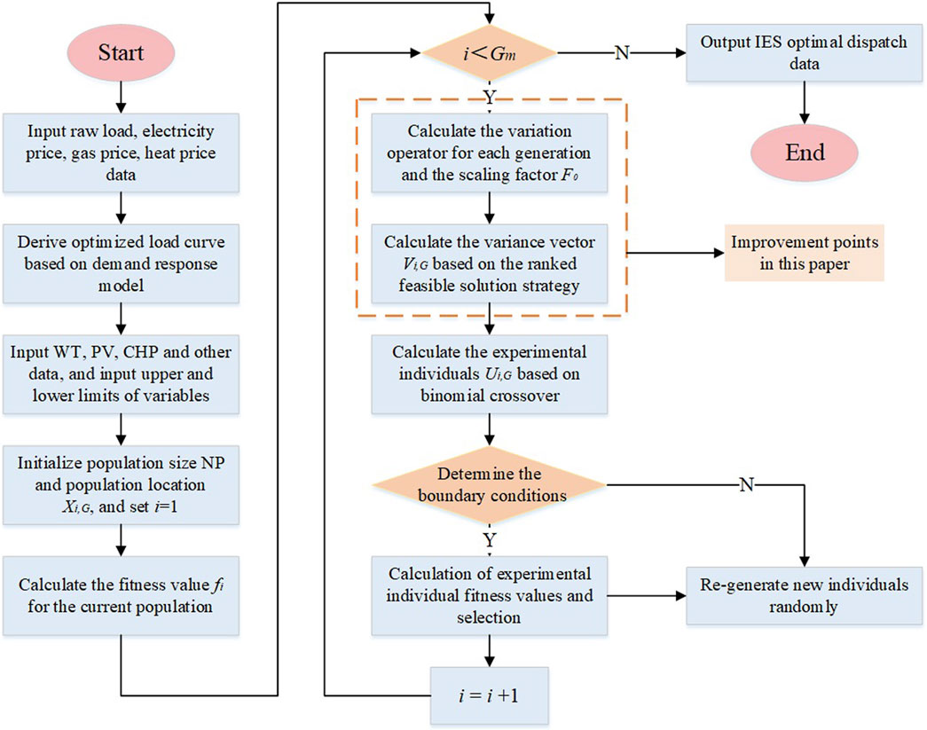
FIGURE 2. Flow chart of improved differential evolution algorithm.
In this paper, the arithmetic simulation is based on the unit equipment parameters and underlying data in the literature (Zhang et al., 2020; Wei et al., 2022; Wang et al., 2020d). The data source for the arithmetic example is a community in Jinan, Northern China. The predicted output of loads, WT, and PV is represented by a typical day of winter in this community. Among them, the WT output, PV output, and electricity, gas, and heat load curves are shown in Figure 3. The parameters of each unit within IESs are shown in Table 1 and Table 2, the peak-valley time electricity price is shown in Table 3(Wei et al., 2022), the electricity price elasticity matrix of IDR is shown in Table 4, the actual carbon emission model parameters are shown in Table 5. Where the natural gas price is taken as 2.55¥/m3, the carbon emission right allowance
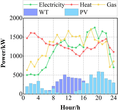
FIGURE 3. The output of PV, WT and Electricity, gas, heat load.
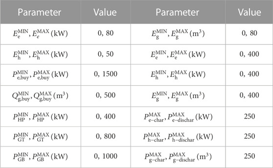
TABLE 1. Parameters of the variables.
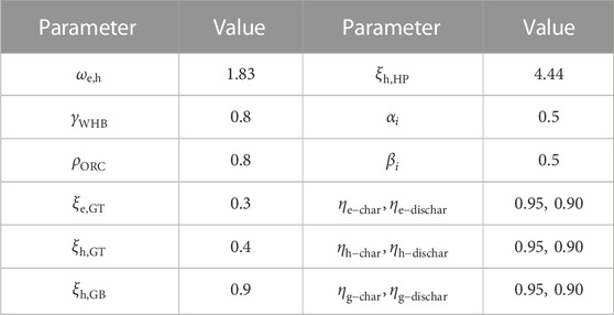
TABLE 2. Parameters of the IES.
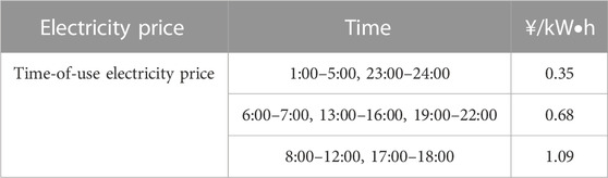
TABLE 3. Electricity price parameters of IES.
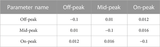
TABLE 4. Electricity price elasticity matrix.
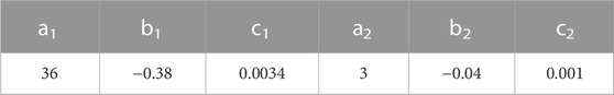
TABLE 5. Parameters of actual carbon emission calculation.
To verify the effectiveness of IESs optimal dispatching considering the stepped carbon trading mechanism and IDR strategy, the following five scenarios are set:
Scenario 1: without considering the stepped carbon trading mechanism and IDR strategy. The IES is optimally dispatched with an improved DE algorithm.
Scenario 2: only considering the IDR strategy, without considering the stepped carbon trading mechanism, The IES is optimally dispatched with an improved DE algorithm.
Scenario 3: only considering the stepped carbon trading mechanism, without considering the IDR strategy, The IES is optimally dispatched with an improved DE algorithm.
Scenario 4: consider the stepped carbon trading mechanism and IDR strategy. The IES is optimally dispatched with a traditional DE algorithm.
Scenario 5: consider the stepped carbon trading mechanism and IDR strategy. The IES is optimally dispatched with a traditional DE algorithm.
The above calculations for IES optimal dispatch were implemented on a PC with MATLAB. The dispatching results of the five scenarios are shown in Table 6, and the power balance diagram in Scenario 5 is shown in Figure 4.
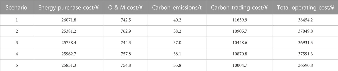
TABLE 6. Comparison of dispatching results under different scenarios.
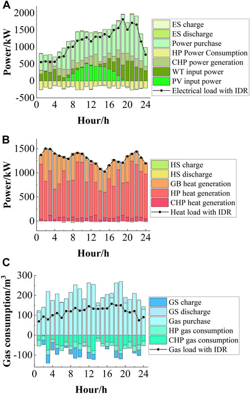
FIGURE 4. The power balance for scenario 5: (A) Electric Power Balance of the IES; (B) Heat Power Balance of the IES; (C) Gas Consumption Balance of the IES.
Comparing Scenario 1 and Scenario 2, since Scenario 1 does not consider the IDR strategy, the multi-energy customers cannot flexibly adjust their energy use strategy according to the price information and actively shift the energy load from the peak price period to the low price period. As a result, the coupling equipment in IESs operates at a high-power state during the peak energy consumption time, which is insufficient to meet the energy demand of customers, thus increasing the demand for purchasing energy from external energy networks. This leads to the generally high carbon transaction cost and operation cost of the IES.
As shown in Table 6, compared with Scenario 1, the total IES operation cost and system carbon emission of Scenario 2 are reduced by 3.65% and 4.98%, respectively. It is verified that the introduction of the IDR strategy can not only realize the economic and optimal operation of the IES but also reduce the carbon emission of the system.
Comparing Scenario 1 and Scenario 3, since Scenario 1 does not consider the stepped carbon trading mechanism, the purchased energy from the upper energy grid is increased during the peak of energy consumption, which leads to the increase of carbon emission of the system. In Scenario 3, since the carbon emission source of the system mainly comes from the power purchase from the upper grid and the coupling equipment, when considering the stepped carbon trading mechanism, the capacity of the units and the power purchase from the grid are enhanced. In this case, the situation of purchasing a large amount of a single energy source in Scenario 1 is avoided. The output of each coupling equipment in the unit is optimized. Thus, the system’s carbon emissions are reduced. Compared with Scenario 1, the total cost of IES operation and system carbon emission of Scenario 3 is reduced by 3.96% and 7.96%, respectively. It is verified that scenario 3 has good carbon reduction capability and economy by considering the stepped carbon trading mechanism.
Comparing Scenario 2 and Scenario 5, since Scenario 5 introduces the stepped carbon trading mechanism and the IDR strategy. The limits of CHP and GB unit output are further strengthened when supplying energy to the multi-energy load after adopting the IDR strategy. The carbon trading mechanism makes the system’s electricity and gas purchases from the upper energy grid to be mutually constrained, thus reducing the carbon emissions of the IES system. Compared with Scenario 2, the total operation cost and system carbon emissions of Scenario 5 are reduced by 1.24% and 6.28%, respectively. Comparing Scenario 3 and Scenario 5, since Scenario 5 not only considers the stepped carbon trading mechanism but also adopts the IDR strategy. On the customer side, it makes multi-energy loads realize peak shaving and multi-energy substitution. While the system shifts the energy load from peak to trough periods, it uses replaceable DR to achieve different low-cost energy sources to meet the demand of multi-energy loads. Together with the synergy of the stepped carbon trading mechanism, the low-carbon economic benefits of the IES are enhanced. Compared with Scenario 2, the total operation cost and system carbon emissions of Scenario 5 are reduced by 0.92% and 3.24%, respectively, which verifies that Scenario 5 can improve the economy of the system while maintaining low-carbon operation by considering the IDR strategy and the stepped carbon trading mechanism.
To verify the advantages of IDR dispatching results, this paper compares the dispatching results of taking the IDR strategy and taking a single curtailable response strategy. As shown in Figure 5. From the figure, each load on the customer side is smoothed to a certain extent. The reason is that after considering the IDR strategy, customers can reasonably adjust their energy usage strategy to meet their energy demand and shift the load from peak times to low times based on time-of-use energy price information. Because of the replaceable DR, customers can satisfy their energy demand by replacing each other with low-cost energy in the same period, which further stimulates the customers to actively participate in the energy adjustment process.
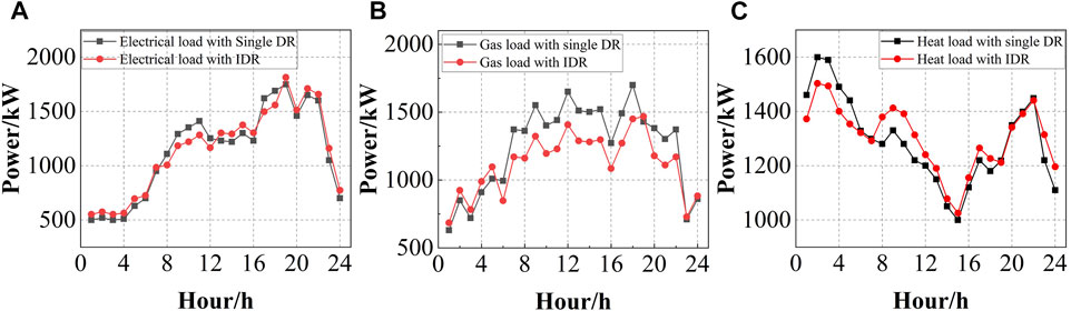
FIGURE 5. The comparison of electricity, gas and heat load participation IDR and single DR: (A) Comparison of IDR and single DR for electrical load; (B) Comparison of IDR and single DR for heat load; (C) Comparison of IDR and single DR for gas load.
For example, in Figure 5A, during the peak times of 9:00–12:00 and 18:00–22:00, the price of electricity is relatively high, so customers voluntarily shift their peak load to the low times of 23:00–6:00, thus playing a role in peak shaving and valley filling. At the same time, due to the effect of replaceable DR in IDR, the cost of electricity is lower than the cost of heat in the 20:00–22:00 time of the electric load, so customers voluntarily convert part of the heat load to electric load in this time. The electric load in the 20:00–22:00 time shows a rising trend. The price DR and substitution DR act simultaneously to cancel each other out, and the heat load which should show an increasing trend remains unchanged at this time.
The peak-to-valley differences before and after the DR of electricity, gas, and heat load decreased by 10.74%, 17.24%, and 7.99%, respectively, and effectively balanced the load fluctuations of customers. In addition, as shown in Table 6, the IDR strategy not only reduces the operating cost of IES but also reduces the amount of energy purchased by the system from the upper energy grid, which effectively reduces the carbon emissions of the IES. The analysis of heat and gas loads is similar and will not be repeated here.
In the stepped carbon trading model, different parameters of the carbon trading mechanism also have an impact on the economic dispatch of IESs, which is analyzed in this paper from three aspects: carbon trading base price, carbon emission interval length and carbon price growth rate. Figure 6 shows the impact of the three parameters on the total operating cost and total carbon emissions of the system.
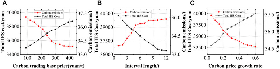
FIGURE 6. Impact of different carbon trading parameters on the system operating cost: (A) Analysis of Carbon trading base price; (B) Analysis of carbon trading interval length; (C) Analysis of carbon trading price growth rate.
As shown in Figure 6A, with the gradual increase of carbon trading base price, the carbon emission of the IES decreases and the total cost of the IES increases. When the carbon trading price is lower than 300 ¥/t, as the carbon trading base price increases, the proportion of carbon trading cost in the total operating cost of IES also rises, and the total operating cost of the IES also rises continuously. In this case, the stronger the binding effect of carbon trading cost, the more the system has to seek a carbon emission balance when purchasing from the upper energy grid. Thus, the carbon emission of the IES is reduced to reduce the carbon trading cost. When the carbon trading base price is greater than 300 ¥/t, the output of each coupling equipment in IESs tends to stabilize as the carbon trading base price increases. The increase in carbon trading base price has less impact on carbon emission, and the carbon emission level tends to be flat. However, the high carbon trading base price will further increase the total operating cost of the system. Therefore, the appropriate carbon trading base price is customized.
As shown in Figure 6B, with the gradual increase of carbon trading interval, the carbon emission of the IES increases, and the total cost of the IES decreases. When the length of the carbon trading interval varies in [0,2], the carbon emissions of the IES are strictly following the stepped carbon trading mechanism to purchase carbon trading credits because the length of the interval is small. it has the greatest constraint on carbon emissions, so the carbon emissions in this interval are the least and the carbon trading cost to be paid is the greatest. When the length of the interval changes in [2,8], the carbon emission interval is larger currently, and due to the existence of load demand within the system, most of the carbon trading costs that the IES need to pay at this time are in the interval with lower costs, the IES constraint for carbon emission decreases. Therefore, the carbon emission of the IES rises rapidly and the system operation cost shows a decreasing trend. When the length of the interval varies [8,12], the longer interval makes the stepped carbon trading mechanism a little different from the traditional one, resulting in most of the system’s carbon emissions buying carbon credits at the base price or very little above the base price. Although the carbon emissions of the system increase, after the interval length is greater than 8, the variation of the interval length has no effect on the carbon emissions, the output of each unit in IESs is in a stable state, and the total operating cost of the system tends to be flat.
As shown in Figure 6C, with the gradual increase of the growth rate of the carbon price, the carbon emissions of the IES decrease, and the total cost of the IES increases. When the price growth rate varies between [0, 0.3], IESs face a higher carbon trading cost, and the IES will reduce the amount of energy purchased from the upper energy grid and adjust the output of each internal unit to reduce the carbon emissions of the system as much as possible. When the price growth rate varies between [0.3, 0.6], the output of each unit of the IES tends to be stable due to the fixed load demand, so the carbon emission gradually tends to be stable. However, due to the large growth rate of carbon trading currently, the total system cost continues to rise.
To sum up, when the carbon trading base price is lower than 300 ¥/t, the length of the carbon emission interval is less than 8t, and the price growth rate is less than 0.3, the carbon emissions of the IES will all decrease to different degrees. When the parameters are larger than the above values, the carbon emissions of the IES will stabilize and bring only the increase in total system cost. Therefore, for IESs, the carbon trading cost and operation cost of the system can be coordinated according to the carbon trading base price, the carbon emission interval length, and the carbon price growth rate. For regulators, by setting reasonable carbon trading parameters, they can achieve reasonable guidance on carbon emissions of production organizations. However, if a high price is set blindly to control carbon emissions, the stepped carbon trading mechanism will be useless.
In this paper, the improved DE algorithm is used to validate and analyze the proposed optimal dispatch model. The improved DE algorithm and the traditional DE algorithm are used to optimize the output of IES under the system considering the IDR strategy and the stepped carbon trading mechanism, respectively. The overall economic efficiency of the system is optimized. Maximum number of iterations is set to 500. Comparing Scenario 4 and Scenario 5, the minimum value of each population change iteration is recorded and the generated adaptation curves are shown in Figure 7, respectively.
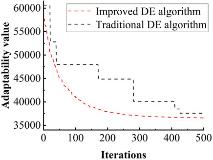
FIGURE 7. Comparison between improved DE algorithm and traditional DE algorithm.
As shown in Figure 7, compared with the traditional DE algorithm, the adaptive operator improved DE algorithm used in this paper has better convergence characteristics and robustness and does not fall into the local optimal solution during the global variational iterations. The algorithm has completely converged to the optimal value in about 400 iterations, and the computation time is 18.741 s. In contrast, the traditional DE algorithm has not converged after 420 iterations and has fallen into the local optimal solution, and does not find the global optimal solution after the iterative variation. This proves that the improved DE algorithm proposed in this paper is feasible and effective.
This paper constructs an IES low carbon optimal dispatch considering the stepped carbon trading mechanism and IDR strategy. In order to verify the results of low carbon economy dispatch of IES, five different scenarios were set up for analysis. The following conclusions can be drawn from the analysis.
1) By introducing price-based DR and substitution-based DR in IESs, the IDR model of electricity, gas, and heat loads is constructed. It enables customers to reasonably adjust their own energy use strategies within a certain satisfaction range, which not only smooths out the load peak-valley differences but also realizes the complementarity and substitution of different loads.
2) In the IES optimal dispatching model, the stepped carbon trading mechanism and the IDR strategy are introduced and compared with the models with only the stepped carbon trading mechanism and only the IDR strategy, respectively. The results show that with the combined effect of the IDR strategy and the stepped carbon trading model, the constraint on IES carbon emissions is more stringent at this time. The model established in this paper effectively reduces the carbon emissions and operation cost of the IES, It improves the economic and environmental benefits of IES effectively.
3) The effects of three coefficients: carbon trading base price, carbon emission interval length, and price growth rate on system carbon emission and total cost are discussed. The results show that the system carbon emission decreases gradually with the increase of the unit carbon trading price, while the total system cost increases rapidly with the increase of the unit carbon trading price, then tends to level off and finally decreases. Setting the appropriate carbon trading parameters plays an important role in the low-carbon operation of IESs.
In the subsequent study, it is necessary to introduce electric-to-gas devices and carbon capture technologies in the structure of IES. Further study of the impact of carbon capture processes in an electric-to-gas device on the optimal dispatch of the IES. Also, there are many uncertainties in the model developed in this paper, and we will consider different timescales (Li and Xu, 2019). This part can be referred to the integrated uncertainty model proposed (Li et al., 2022). The specific uncertainties in the generation side and demand side are modeled as an interval range instead of fixed values. This consideration makes the optimal dispatch of IES more realistic. Finally, we also want to model multiple IESs connected to the grid. Based on a comprehensive consideration of the cooperative and competitive relationships between different systems and different energy suppliers (Li et al., 2023), we will analyze the optimal scheduling results of each system.
The raw data supporting the conclusions of this article will be made available by the authors, without undue reservation.
XY: Conceptualization, Methodology, Software, Data curation, Visualization, Writing−original draft. ZJ: Funding acquisition, Conceptualization, Methodology, Visualization, Validation, Writing−review and editing. JX: Data curation, Methodology. XL: Conceptualization, Methodology. All authors contributed to the article and approved the submitted version.
This work was financially supported by the National Natural Science Foundation of China under Grant 52107100 and 52077035, the Natural Science Foundation of Jiangsu Province of China under Grant BK20190710, and the Key Research and Development Program of Jiangsu Province under Grant BE2020081-4.
The authors declare that the research was conducted in the absence of any commercial or financial relationships that could be construed as a potential conflict of interest.
The Supplementary Material for this article can be found online at: https://www.frontiersin.org/articles/10.3389/felec.2023.1110039/full#supplementary-material
Cao, Y., Kang, Z., Bai, J., Cui, Y., Chang, I. S., and Wu, J. (2022). How to build an efficient blue carbon trading market in China? - a study based on evolutionary game theory. J. Clean. Prod. 367. doi:10.1016/j.jclepro.2022.132867
Cheng, Y. H., Zhang, N., Zhang, B. S., Kang, C. Q., Xi, W. M., and Feng, M. S. (2019). Low-carbon operation of multiple energy systems based on energy-carbon integrated prices. IEEE Trans. Smart Grid 11 (2), 1307–1318. doi:10.1109/TSG.2019.2935736
Gu, W., Wang, J., Lu, S., Luo, Z., and Wu, C. (2017). Optimal operation for integrated energy system considering thermal inertia of district heating network and buildings. Appl. Energy 199, 234–246. doi:10.1016/j.apenergy.2017.05.004
Guo, R., Ye, H., and Zhao, Y. (2022). Low carbon dispatch of electricity-gas-thermal-storage integrated energy system based on stepped carbon trading. Energy Rep. 8, 449–455. doi:10.1016/j.egyr.2022.09.198
Hu, H., Wen, L., and Zheng, K. (2021). “Low carbon economic dispatch of multi-energy combined system considering carbon trading,” in 2021 11th International Conference on Power and Energy Systems (ICPES), Shanghai, China, 18-20 December 2021, 838–843. doi:10.1109/ICPES53652.2021.9683862
Ihsan, A., Jeppesen, M., and Brear, M. J. (2019). Impact of demand response on the optimal, techno-economic performance of a hybrid, renewable energy power plant. Appl. Energy 238, 972–984. doi:10.1016/j.apenergy.2019.01.090
Li, P., Wang, Z., Wang, N., Yang, W., Li, M., Zhou, X., et al. (2021). Stochastic robust optimal operation of community integrated energy system based on integrated demand response. Int. J. Electr. Power & Energy Syst. 128, 106735. doi:10.1016/j.ijepes.2020.106735
Li, Y., Tang, W., and Wu, Q. (2019). “Modified carbon trading based low-carbon economic dispatch strategy for integrated energy system with CCHP,” in 2019 IEEE Milan PowerTech, Milan, Italy, 23-27 June 2019, 1–6. doi:10.1109/PTC.2019.8810482
Li, Z. M., Wu, L., Xu, Y., Wang, L. H., and Yang, N. (2023). Distributed tri-layer risk-averse stochastic game approach for energy trading among multi-energy microgrids. microgrids 331, 120282. doi:10.1016/j.apenergy.2022.120282
Li, Z. M., Wu, L., Xu, Y., and Zheng, X. D. (2022). Stochastic-weighted robust optimization based bilayer operation of a multi-energy building microgrid considering practical thermal loads and battery degradation. IEEE Trans. Sustain. Energy 13 (2), 668–682. doi:10.1109/TSTE.2021.3126776
Li, Z. M., and Xu, Y. (2019). Temporally-coordinated optimal operation of a multi-energy microgrid under diverse uncertainties. Appl. Energy 240, 719–729. doi:10.1016/j.apenergy.2019.02.085
Liu, P., Ding, T., Zou, Z., and Yang, Y. (2019). Integrated demand response for a load serving entity in multi-energy market considering network constraints. Appl. Energy 250, 512–529. doi:10.1016/j.apenergy.2019.05.003
Luo, Z., Hong, S., and Ding, Y. (2019). A data mining-driven incentive-based demand response scheme for a virtual power plant. Appl. Energy 239, 549–559. doi:10.1016/j.apenergy.2019.01.142
Lynch, M. Á., Nolan, S., Devine, M. T., and O’Malley, M. (2019). The impacts of demand response participation in capacity markets. Appl. Energy 250, 444–451. doi:10.1016/j.apenergy.2019.05.063
Ma, X., Liang, Y., Wang, K., Jia, R., Wang, X., Du, H., et al. (2022). Dispatch for energy efficiency improvement of an integrated energy system considering multiple types of low carbon factors and demand response. Front. Energy Res. 10. doi:10.3389/fenrg.2022.953573
Mi, X. (2022). Multi-objective variation differential evolutionary algorithm based on fuzzy adaptive sorting. Energy Rep. 8, 1020–1028. doi:10.1016/j.egyr.2022.10.333
Qiu, B., Song, S. X., Wang, K., and Yang, Z. (2022). Optimal operation of regional integrated energy system considering demand response and ladder-type carbon trading mechanis. Proc. CSU-EPSA. 34 (05), 87–95+101. doi:10.19635/j.cnki.csu-epsa.000869
Wang, Y. Q., Qiu, J., Tao, Y. C., Zhang, X., and Wang, G. B. (2020c). Low-carbon oriented optimal energy dispatch in coupled natural gas and electricity systems. Appl. Energy 280, 115948. doi:10.1016/j.apenergy.2020.115948
Wang, B., Sun, H., and Song, X. (2022). Optimal dispatching modeling of regional power–heat–gas interconnection based on multi-type load adjustability. Front. Energy Res. 10. doi:10.3389/fenrg.2022.931890
Wang, H. Y., Li, K., Zhang, C. H., and Ma, X. (2020d). Distributed Coordinative Optimal Operation of Community Integrated Energy System Based on Stackelberg Game. Proceedings of the CSEE 40 (17), 5435–5445. doi:10.13334/j.0258-8013.pcsee.200141
Wang, J., Zhong, H., Ma, Z., Xia, Q., and Kang, C. (2017). Review and prospect of integrated demand response in the multi-energy system. Appl. Energy 202, 772–782. doi:10.1016/j.apenergy.2017.05.150
Wang, L., Dong, H., Lin, J., and Zeng, M. (2022). Multi-objective optimal scheduling model with IGDT method of integrated energy system considering ladder-type carbon trading mechanism. Int. J. Electr. Power & Energy Syst. 143, 108386. doi:10.1016/j.ijepes.2022.108386
Wang, Y. Q., Ma, Y., Song, F., Ma, Y., Qi, C., Huang, F., et al. (2020a). Economic and efficient multi-objective operation optimization of integrated energy system considering electro-thermal demand response. Energy 205, 118022. doi:10.1016/j.energy.2020.118022
Wang, Y. Q., Qiu, J., Tao, Y. C., and Zhao, J. H. (2020b). Carbon-Oriented operational planning in coupled electricity and emission trading markets. IEEE Trans. Power Syst. 35 (4), 3145–3157. doi:10.1109/TPWRS.2020.2966663
Wang, Y., Yu, H., Yong, M., Huang, Y., Zhang, F., and Wang, X. (2018). Optimal scheduling of integrated energy systems with combined heat and power generation, photovoltaic and energy storage considering battery lifetime loss. Photovolt. Energy Storage Considering Battery Lifetime Loss 11 (7), 1676. doi:10.3390/en11071676
Wei, Z. B., Ma, X. R., Guo, Y., Wei, P. N., Lu, B. W., and Zhang, H. T. (2022). Optimized operation of integrated energy system considering demand response under carbon trading mechanism. Electr. Power Constr. 43 (01), 1–9. doi:10.12204/j.issn.1000-7229.2022.01.001
Wu, M., Du, P., Jiang, M., Goh, H. H., Zhu, H., Zhang, D., et al. (2022). An integrated energy system optimization strategy based on particle swarm optimization algorithm. Energy Rep. 8, 679–691. doi:10.1016/j.egyr.2022.10.034
Xiong, Z., Luo, S., Wang, L., Jiang, C., Zhou, S., and Gong, K. (2022). Bi-level optimal low-carbon economic operation of regional integrated energy system in electricity and natural gas markets. Front. Energy Res. 10, 959201. doi:10.3389/fenrg.2022.959201
Zhang, H., Sun, K., Yang, P., Yu, D., Weng, H., and Zhou, H. (2021). “Optimal day-ahead dispatch of integrated energy systems with carbon emission considerations,” in 2021 IEEE Sustainable Power and Energy Conference (iSPEC), Nanjing, China, 23-25 December 2021, 2190–2195. doi:10.1109/iSPEC53008.2021.9735958
Zhang, Y., Huang, Z., Zheng, F., Zhou, R., An, X., and Li, Y. (2020). Interval optimization based coordination scheduling of gas–electricity coupled system considering wind power uncertainty, dynamic process of natural gas flow and demand response management. Energy Rep. 6, 216–227. doi:10.1016/j.egyr.2019.12.013
IES integrated energy system
DR demand response
IDR Integrated Demand Response
CL curtailable load
SL shiftable load
RL replaceable load
WT Wind Turbine
PV Photovoltaic
CHP combined heat and power
GT gas turbine
WHB waste heat boiler
ORC organic Rankine cycle
DE differential evolution
O&M operation and maintenance
Keywords: integrated demand response, stepped carbon trading, integrated energy system, carbon emission, differential evolution algorithm
Citation: Ye X, Ji Z, Xu J and Liu X (2023) Optimal dispatch of integrated energy systems considering integrated demand response and stepped carbon trading. Front. Electron. 4:1110039. doi: 10.3389/felec.2023.1110039
Received: 28 November 2022; Accepted: 13 February 2023;
Published: 23 February 2023.
Edited by:
Zhengmao Li, Nanyang Technological University, SingaporeReviewed by:
Yongli Wang, North China Electric Power University, ChinaCopyright © 2023 Ye, Ji, Xu and Liu. This is an open-access article distributed under the terms of the Creative Commons Attribution License (CC BY). The use, distribution or reproduction in other forums is permitted, provided the original author(s) and the copyright owner(s) are credited and that the original publication in this journal is cited, in accordance with accepted academic practice. No use, distribution or reproduction is permitted which does not comply with these terms.
*Correspondence: Zhenya Ji, NjEyMTRAbmpudS5lZHUuY24=
Disclaimer: All claims expressed in this article are solely those of the authors and do not necessarily represent those of their affiliated organizations, or those of the publisher, the editors and the reviewers. Any product that may be evaluated in this article or claim that may be made by its manufacturer is not guaranteed or endorsed by the publisher.
Research integrity at Frontiers
Learn more about the work of our research integrity team to safeguard the quality of each article we publish.