Subdivision of river channel sand micro-scale facies with feature attention spatio-temporal network

Introduction: Sedimentary micro-scale facies research is essential for characterizing the lateral and vertical evolutionary patterns and contact relationships within sedimentary facies. This is critical for the redevelopment of high-water-cut oil reservoirs. The complexity of river channel sands, including their horizontal and vertical heterogeneity, well connectivity, and the effectiveness of water injection, necessitates a more refined subdivision of sedimentary facies. Traditional manual identification methods are labor-intensive and prone to subjectivity, highlighting the need for a more automated and precise solution.

Methods: This paper integrates well-logging sedimentology with statistical theory, selecting multiple reservoir and logging parameters to establish a new classification standard for river channel sand sedimentary micro-scale facies. Based on deep learning techniques, we propose a network that combines feature attention and spatio-temporal feature extraction. The feature attention module dynamically assigns weights to logging parameters based on their correlation with the target classification, enhancing the contribution of key parameters to the classification task. Meanwhile, the spatio-temporal feature extraction module fully leverages spatial and sequential information from the logging data, enabling precise identification of river channel sand sedimentary micro-scale facies.

Results: This method, applied to a real-world oilfield for residual oil development, subdivides deltaic river channel sand sedimentary micro-scale facies into four distinct types. It improves overall accuracy by 8% compared to traditional CNN models and significantly outperforms existing machine learning methods. Notably, the method achieves 100% classification accuracy for certain micro-facies categories, with an overall classification accuracy of 94.9%, demonstrating its superior performance and potential for application in complex sedimentary environments.

Discussion: This approach not only enhances the accuracy of sedimentary micro-scale facies classification but also offers a new framework for analyzing the connectivity between injection and production well groups. The integration of spatio-temporal feature extraction with feature attention significantly improves model performance, especially in the complex, heterogeneous environments typical of river channel sands. This method represents a substantial improvement over traditional models and has broad applicability in the field of reservoir management.

1 Introduction

As oilfield development technologies continue to advance, challenges such as the rapid decline in oil and gas production and the gradual increase in water cut have become increasingly prominent (Li et al., 2013; Song, 2023). Complex factors such as difficulties in understanding enrichment patterns, well connectivity, and reservoir heterogeneity remain major constraints in the development of remaining oil reserves (Shu et al., 2017). Since the distribution of sedimentary micro-scale facies directly influences the distribution of oil and gas, studying these micro-scale facies is essential for guiding the spatial analysis of remaining oil enrichment and production prediction (Luo et al., 2022; Peng and Guo, 2023). Consequently, sedimentary micro-scale facies analysis and intelligent identification have emerged as pivotal components in oil and gas exploration and development.

Well-logging data, which is rich in geological sedimentary information (Kaakinen et al., 2009), serves as a critical foundation for sedimentary micro-scale facies identification. However, accurately delineating the boundaries of different sedimentary micro-scale facies remains a significant challenge, especially during the water injection development phase, where severe horizontal and vertical heterogeneity exists within the channel sands of oil reservoirs. There is an urgent need to conduct detailed geological studies of thick oil reservoirs, identify the contact patterns of river channels with different depositional origins, and clarify the connectivity between injection and production well groups. Achieving these objectives requires further subdivision and intelligent recognition of river channel sand sedimentary micro-scale facies.

Traditional machine learning techniques, such as support vector machines (SVMs) (Liu et al., 2020), fuzzy clustering neural networks (Zhang, 2013), and backpropagation (BP) neural networks (Tang, 2023), have been widely used for automatic identification of sedimentary micro-scale facies. Fuzzy clustering, often enhanced with expert input, is used for facies classification based on specific needs (Cherana et al., 2022), but is sensitive to noise and outliers, limiting generalization. SVMs, which use statistical theory for lithofacies prediction (Wang et al., 2019), improve accuracy but struggle with large-scale data and inefficient parameter optimization. BP neural networks combined with principal component analysis (PCA) (Li et al., 2017; Zhang, 2013) enhance accuracy and efficiency, yet suffer from sensitivity to initial weights and instability. Self-organizing neural networks (Zhang K. et al., 2022) reduce training iterations and time costs in facies identification.

Despite their successes, traditional machine learning methods are limited by their reliance on linear relationships between inputs and targets, effectively handling redundant structures but failing to capture the complex non-linear relationships in logging data (Hou et al., 2020). They also neglect trends and correlations with geological depth (Zeng et al., 2022), restricting their ability to extract deep non-linear information and retain historical data, thereby impacting generalization and learning efficiency.

Deep learning has become essential for extracting nonlinear features in heterogeneous reservoirs, improving model performance through structural and parameter optimizations (de Lima et al., 2020; Shengli et al., 2016; Zhang H. et al., 2022). Convolutional Neural Networks (CNNs), with their weight-sharing and pooling capabilities, enable efficient extraction of spatial information from logging parameters (Guo and Zhu, 2019; Song et al., 2022; de Lima et al., 2020), reducing redundancy and overfitting. Parameters like natural gamma and resistivity serve as direct inputs for one-dimensional CNNs, achieving high accuracy in sedimentary micro-scale facies identification (Imamverdiyev and Sukhostat, 2019). Twin CNNs (Feng et al., 2019) and U-Net architectures (Liu et al., 2022) transform lithofacies interpretation into supervised image tasks, capturing global and local texture features in rock images (Zhu et al., 2018). CNN-based models offer higher accuracy and faster computation than traditional methods. Recurrent Neural Networks (RNNs) use memory units to leverage temporal information from logging data, improving lithofacies identification accuracy (Choi et al., 2020; dos Santos et al., 2021; Chen et al., 2021; Tian and Verma, 2022). Given the continuity of petrographic profiles in the field, sensitivity analyses are often performed on logging parameters like natural gamma and bulk density. Long Short-Term Memory (LSTM) networks are then used for lithofacies classification, analyzing vertical correlations along the reservoir (Khan and Kirmani, 2024), while Gated Recurrent Unit (GRU) networks, simplifying the LSTM design, are more effective for small datasets (Feng, 2024).

While single deep neural networks can model the nonlinear relationships between logging parameters, their ability to refine both spatial and temporal features of reservoir attributes remains limited, often resulting in poor generalizability and stability. For example, CNNs may overlook sequential correlations between sedimentary micro-scale facies and logging parameters at depth, failing to accurately capture vertical geological features during identification processes. Although RNNs are adept at capturing these sequential correlations, their single-layer networks exhibit limited feature extraction capabilities, and deeper networks are prone to degradation issues (Aslam et al., 2020). Moreover, directly training neural networks with raw logging parameters often fails to fully exploit the rich information contained in logging data, making it difficult to capture the complex geological structures and variations in log parameter waveforms, such as shape and amplitude (Luo et al., 2022). These limitations hinder significant advancements in the precise classification of sedimentary micro-scale facies. Table 1 summarizes the advantages, disadvantages, and application scenarios of previous methods for sedimentary micro-scale facies identification as well as the proposed method in this study.

Table 1

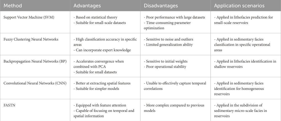
Table 1. Comparison of methods for sedimentary micro-scale facies identification.

Based on the analysis of existing approaches, this paper proposes a novel intelligent identification method for channel sand sedimentary micro-scale facies–the Feature Attention and Spatio-Temporal Network (FASTN). Traditional methods often struggle to capture the complex non-linear relationships between logging parameters and sedimentary facies, limiting their ability to fully characterize sedimentary features, particularly in heterogeneous reservoirs. In contrast, the proposed method overcomes these limitations by integrating both spatial and temporal features of logging data, providing a more detailed and accurate identification of sedimentary micro-scale facies. A key innovation of this method is the feature attention mechanism, which dynamically assigns greater weight to features that are more relevant to the classification results, ensuring that critical information is prioritized and irrelevant or noisy data is downweighted. The method begins by combining logging sedimentology with statistical theories to establish a model for subdividing channel sand facies, selecting optimal parameters and constructing new neural network inputs based on these features. By leveraging a combination of Convolutional Neural Networks (CNNs) and Long Short-Term Memory (LSTM) networks, enhanced with this attention mechanism, the model effectively captures and refines spatiotemporal information. Finally, the method is validated in various residual oil development fields, showing an 8% improvement in accuracy over traditional CNN-based models. This highlights the ability of the method to enhance sedimentary facies identification through more targeted and effective spatiotemporal analysis.

2 Logging sedimentary micro-scale facies pattern

2.1 Study area overview

The study area is situated in the Songliao Basin, a large intracontinental rift basin located in the central part of northeast China. The Yaojia Formation, part of the Upper Cretaceous system, is dominated by deltaic deposits and represents a critical interval for hydrocarbon exploration in the basin (Figure 1). The target stratum in the study area belongs to delta front facies deposits (Yang et al., 2005; 2022), influenced by the dual hydrodynamic forces of rivers and lake waves. It is characterized by straight, narrow distributary channels that are heavily incised and laterally stacked. Additionally, abandoned channels and discontinuous inter-channel deposits are scattered throughout the area, predominantly arranged in a mesh-like or dendritic pattern. The drilling encounter rate for channel sands is approximately 30%–40%, with widths ranging from 100 to 300 m and an average channel thickness of 3.0 m. As the continuity of the channel sands diminishes, the well network’s control over the sand bodies weakens, and inter-channel sand bodies are interspersed in flaky or strip-like patterns along channel margins, without forming extinction zones.

Figure 1

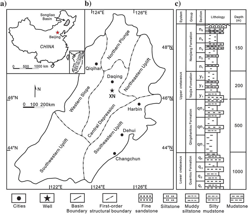
Figure 1. (A) The geographical location of the Songliao Basin in China. (B) The structural framework of the study area and the location of well XN within it. (C) The stratigraphic column of the study area, illustrating the formations, lithology, and depth distribution.

Analysis of the channel sand depositional profiles (Figure 2) reveals significant differences in thickness and hydrodynamic conditions across different parts of the same channel. The channels consist of geomorphic units such as incised zones, active channels, channel margins, and abandoned channels, each with distinct geological characteristics. These differences result in significant variations in reservoir quality, further intensifying the lateral and vertical heterogeneity of the reservoirs. Currently, with 399 oil wells completed, the study area has entered the polymer flooding stage, and the remaining oil exhibits highly dispersed patterns with localized enrichment, especially in areas with poor reservoir connectivity. The complexity of inter-well connectivity and uneven effectiveness highlights the necessity of refining the subdivision of channel sand sedimentary micro-scale facies. Investigating the connectivity differences among these geological units will aid in accurately evaluating reservoir potential and provide a scientific basis for designing customized strategies for remaining oil recovery.

Figure 2

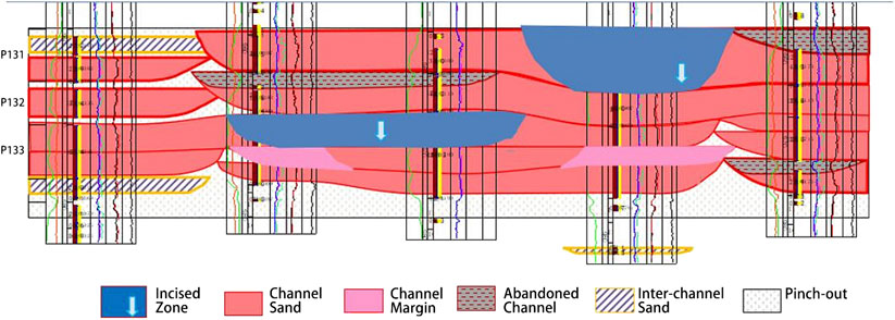
Figure 2. The channel sand depositional profiles, showing variations in thickness and hydrodynamic conditions across different geomorphic units.

2.2 Criteria for sedimentary micro-scale facies classification

There is no direct correspondence between logging facies and sedimentary micro-scale facies, particularly because paleontological and geochemical indicators are often challenging to derive from logging data. This study, centered on core-calibrated logging, aims to establish the relationship between sedimentary subfacies and micro-scale facies identification under sedimentary facies calibration through statistical analysis and knowledge-based reasoning. As a result, a sedimentary micro-scale facies-logging facies interpretation model is developed to provide standards for further subdivision of channel sand sedimentary micro-scale facies.

Core wells and representative basic wells along the main trunk are selected to examine the well log characteristics of sedimentary micro-scale facies. Given the multifactorial nature of sedimentary micro-scale facies identification, a single well log parameter is insufficient to fully characterize a sedimentary micro-scale facies unit. Therefore, this study focuses on analyzing river channel sand facies samples from 15 closed-core wells and 51 basic trunk wells within the study area. Definitions and key abbreviations related to the analysis are summarized in Table 2. A detailed investigation is conducted into the relationships between well logging parameters, including spontaneous potential (SP), gamma ray (GR), micro-normal resistivity (Rmn), formation thickness (fth), and effective thickness (eth), with sedimentary micro-scale facies. In previous studies, effective thickness and the effective thickness/formation thickness ratio have been used to distinguish different sedimentary facies. However, when subdividing sedimentary microfacies within a single facies, these two parameters tend to overlap significantly, making it difficult to effectively differentiate between the microfacies. Therefore, we introduce Rmn-GS as a new parameter to further subdivide channel sand sedimentary microfacies, enhancing the accuracy of microfacies identification.

Table 2

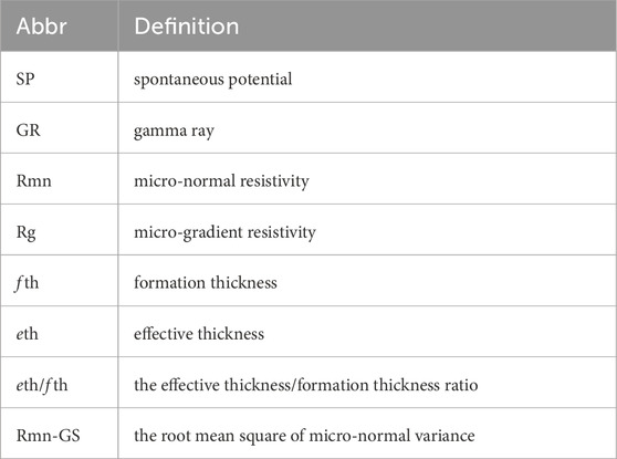
Table 2. Important abbreviations list.

Resistivity micro-logging includes two electrode systems: micro-gradient and micro-potential. The micro-gradient electrode system has a smaller detection range and mainly reflects the resistivity of the mud cake on the borehole wall, while the micro-potential electrode system has a larger detection range, primarily reflecting the resistivity of the wash zone. In permeable formations, mud filtrate infiltration during drilling leads to the formation of a mud cake with lower resistivity than the surrounding wash zone. Consequently, the micro-gradient and micro-potential curves exhibit a positive difference. Micro-electrode logging offers the highest vertical resolution in conventional logging, reaching up to 0.2 m, which makes it capable of capturing subtle water flow fluctuations during the deposition of channel sand sedimentary micro-scale facies.

Since the development of the Daqing oilfield, micro-electrode logging has been widely used for open-hole logging measurements, making the micro-potential logging curve an optimal parameter for the subdivision of channel sand sedimentary micro-scale facies. To reflect the smoothness of the well logging curve, the root mean square of the variance (variance root parameter) is employed. Combining logging sedimentology and statistical theory, the effective thickness (eth) of the study area is selected, along with the effective thickness/formation thickness ratio (eth/fth) and the root mean square of micro-normal variance (Rmn-GS), as key well log features to represent sedimentary micro-scale facies. The root mean square of the micro-potential variance reflects the degree of dentate morphology in sedimentary micro-scale facies sections: the larger the value, the more pronounced the dentate features. This parameter is calculated using Equation 1.

$GS={\left(G_1+S^2\right)}^{\frac{1}{2}}=\sqrt{\frac{{\sum }_{i=1}^{M\left(h\right)}{\left(Y\left(i\right)-Y\left(i+h\right)\right)}^2}{2M\left(h\right)}+\frac{{\sum }_{i=1}^N{\left(Y\left(i\right)-V\right)}^2}{N-1}}(1)$

where, $G_1=\frac{{\sum }_{i=1}^{M(h)}{\left(Y(i)-Y(i+h)\right)}^2}{2M(h)}$ represents the variance function of the logging data $[Y(i),Y(i+h)]$ with a step size of $h$, capturing local changes at the microscopic scale, and $M(h)$ denotes the number of observations for local changes with a step size of $h$. Similarly, $S^2=\frac{{\sum }_{i=1}^N{\left(Y(i)-V\right)}^2}{N-1}$ reflects the variance function of the overall changes during this stage, where $N$ is the total number of observed data points throughout the entire stage.

By comparing the characteristics of the Rmn-GS curves, the channel sand facies in the study area are further subdivided into four types of sedimentary micro-scale facies, as detailed in Table 3. The crenulation degree progressively increases from Class I to Class III, with Class IV channel sands exhibiting the highest degree of crenulation among all types. The logging curve characteristics corresponding to each sedimentary micro-scale facies type are illustrated in Figure 3.

Table 3

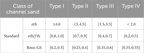
Table 3. Classification criteria of channel sand sedimentary micro-scale facies (m).

Figure 3

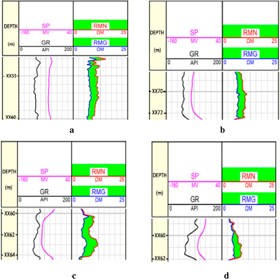
Figure 3. Sedimentary micro-scale facies log curve characteristics. (a) Type I (Incised Zone), (b) Type II (Channel Sand), (c) Type III (Inter-channel Sand), (d) Type IV (Abandoned Channel).

For class I channel sand sedimentary micro-scale facies (Figure 3a, Incised Zone), the Rmn-GS curve typically exhibits high or extremely high amplitude characteristics, with moderate to thick layers. The micro-electrode and micro-potential curves display a characteristic thick box shape, marked by a sharp increase at the base and a gradual-to-sharp transition at the top. The amplitude difference between extremely high and high values is significant, and the curve morphology is generally smooth. The effective thickness is greater than or equal to 4.0 m, while the ratio of effective thickness to formation thickness ranges from 0.8 to 1.0.

For class II channel sand sedimentary micro-scale facies (Figure 3b, Channel Sand), the Rmn-GS curve also demonstrates high or extremely high amplitude characteristics, with moderate layer thicknesses. The micro-electrode and micro-potential curves show a typical bell-shaped or thick box-shaped form, featuring a sharp increase at the base and a gradual-to-sharp transition at the top. The amplitude difference between extremely high and high values remains significant, and the curve morphology transitions from smooth to slightly dentate. The effective thickness ranges from 3.0 to 4.5 m, with the effective thickness-to-formation thickness ratio between 0.7 and 0.9.

For class III channel sand sedimentary micro-scale facies (Figure 3c, Inter-channel Sand), the Rmn-GS curve continues to exhibit high or extremely high amplitude characteristics, but with fine to medium layers. The micro-electrode and micro-potential curves display a bell-shaped, thick box-shaped, or thin box-shaped form, characterized by a sharp increase at the base and a gradual-to-sharp transition at the top. The amplitude difference between extremely high and high values remains significant, and the curve morphology ranges from smooth to dentate. The effective thickness falls between 1.5 and 3.5 m, with the effective thickness-to-formation thickness ratio ranging from 0.4 to 0.7.

For class IV channel sand sedimentary micro-scale facies (Figure 3d, Abandoned Channel), the Rmn-GS curve consistently exhibits high or extremely high amplitude characteristics, with fine layers. The micro-electrode and micro-potential curves are bell-shaped or thin box-shaped, featuring a sharp increase at the base and a gradual-to-sharp transition at the top. The amplitude difference between extremely high and high values is significant, and the curve morphology ranges from smooth to dentate. The effective thickness is less than or equal to 2.0 m, and the effective thickness-to-formation thickness ratio ranges from 0.2 to 0.55.

2.3 Dataset and preprocessing

According to the subdivision standards for channel sand sedimentary micro-scale facies, 15 tightly spaced core wells and 51 main wells within the study area are selected as research subjects to construct a logging dataset. This dataset comprises parameters such as effective thickness (eth), the ratio of effective thickness to formation thickness (eth/fth), the root mean square of micro-potential variance (Rmn-GS), and channel sand facies characteristics. The dataset is divided into a training set accounting for 80%, and a test set accounting for the remaining 20%. Detailed information about the test set is provided in Table 4.

Table 4

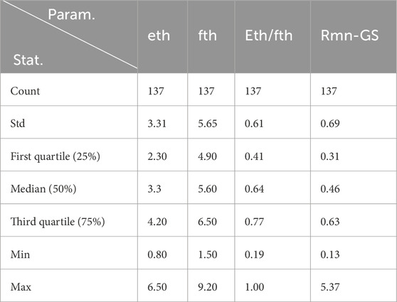
Table 4. Test set data condition.

Figure 4 illustrates the distribution of actual channel sand facies samples in the test set. In the figure, I represents incised zone (Class I), II represents channel sand (Class II), III represents inter-channel sand (Class III), and IV represents abadoned channel (Class IV). The test set comprises 25 samples of incised zone, 28 samples of channel sand, 55 samples of inter-channel sand, and 29 samples of abadoned channel.

Figure 4

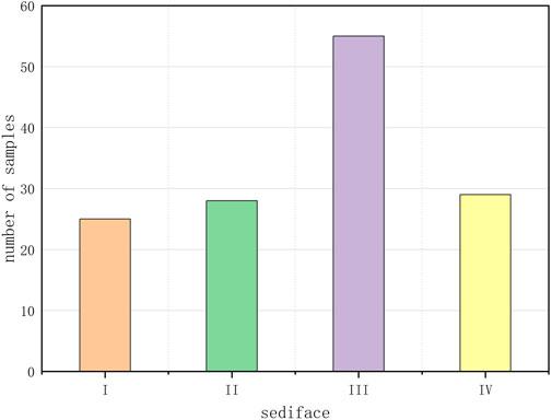
Figure 4. Percentage composition of sedimentary micro-scale facies in the test set.

The Maximum Information Coefficient (MIC) is employed to evaluate the linear relationships between sedimentary micro-scale facies and their associated logging parameters (Cao et al., 2021). As illustrated in Figure 5, the correlation coefficients between channel sand sedimentary micro-scale facies and the parameters effective thickness (eth), formation thickness (fth), root mean square of micro-potential variance (Rmn-GS), and the ratio of effective thickness to formation thickness (eth/fth) are 0.38, 0.24, 0.49, and 0.35, respectively. These relatively weak relationships, coupled with the inherent heterogeneity of reservoir structures, present significant challenges for accurately predicting channel sand sedimentary micro-scale facies.

Figure 5

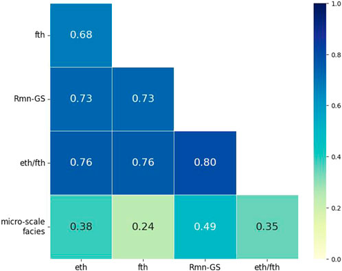
Figure 5. Relationships between classes of channel sand sedimentary micro-scale facies and logging parameters, quantified using the Maximum Information Coefficient (MIC).

3 Methods

3.1 Model design

This section proposes the Feature Attention and Spatio-Temporal Network (FASTN). The model combines the feature attention mechanism with convolutional neural network and long short term memory recurrent neural network (LSTM) to realize intelligent recognition of channel sand sedimentary micro-scale facies. The network architecture is illustrated in Figure 6.

Figure 6

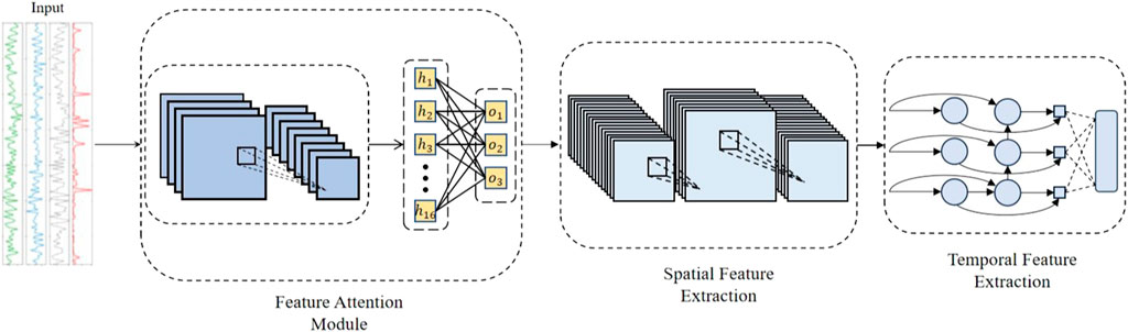
Figure 6. The architecture of the sedimentary micro-scale facies intelligent identification model FASTN. The model takes several characteristic parameters as input and outputs the probabilities of lithofacies categories.

The FASTN model utilizes three feature parameters as input data: effective thickness, the ratio of effective thickness to formation thickness (eth/fth), and Rmn-GS. The model is composed of three main modules: the Feature Attention (FAtt) module, the Spatial Features (SF) module, and the Temporal Features (TF) module. Its primary focus is the extraction of key logging features for sedimentary micro-scale facies classification.

Firstly, the FAtt module calculates and assigns similarity weights between the target and the input logging parameters, enabling the model to emphasize logging data that is more relevant to the target. By weighting the input data, this module not only enhances focus on critical features but also reduces training time and improves model accuracy. Secondly, the SF module employs multiple localized and sliding filters to capture multi-scale spatial features across different logging parameters. Subsequently, the TF module, based on the LSTM network, integrates current and neighboring temporal information to extract essential temporal features. Finally, the fully connected layer processes the extracted features to output the probabilities of lithofacies categories, enabling the intelligent classification of sedimentary micro-scale facies.

To address the challenges in the subdivision of sedimentary micro-scale facies, the FASTN model incorporates several key innovations:

1. Feature Attention Mechanism: By weighting the input features, the model focuses on the most relevant geological features for the recognition of sedimentary micro-scale facies, improving classification accuracy and reducing training time while minimizing noise interference.

2. Joint Extraction of Spatial and Temporal Features: The Spatial Features (SF) module captures spatial variations using multi-scale filters, enhancing the model’s ability to recognize spatial differences in strata, while the Temporal Features (TF) module, based on LSTM, handles time-dependent relationships and improves classification precision by capturing temporal changes in the strata.

3. Multi-Level Feature Fusion: FASTN integrates feature attention, spatial, and temporal features to extract key information from multiple perspectives, addressing the limitations of traditional methods in handling complex geological features.

These innovations enable FASTN to effectively perform sedimentary micro-scale facies recognition, solving the high-dimensional complexity in sedimentary micro-scale facies subdivision and providing a more accurate solution for sedimentary micro-scale facies identification.

3.2 Feature attention module

Directly using raw data as input for neural networks treats all parameters as equally important due to the lack of feature selection or preprocessing, which disregards the varying significance of different parameters to the identification target. This approach may increase the storage requirements for high-dimensional data, reduce computational efficiency, and make it difficult to effectively extract nonlinear and complex key features, potentially impacting the identification accuracy. Inspired by the human brain’s signal processing mechanism (Cowan, 2001), the attention mechanism addresses this issue by dynamically adjusting the weighting of information. It measures the similarity between the identification target and the input data, assigning greater weights to parameters with higher relevance. This enables more accurate predictions, reduces storage space requirements, and optimizes computational efficiency.

To tackle the limitation that CNN does not explicitly assign feature importance, this study integrates an attention mechanism with CNN to construct a feature attention module. While CNN can automatically learn spatial and hierarchical patterns through convolutional filters, it does not inherently distinguish the relative importance of different input features at a global level. The proposed module, as illustrated in Figure 7, explicitly assigns adaptive weights to input parameters based on their correlation with the target representation, ensuring that more relevant logging data receives higher emphasis.

1. CNN Layer: The CNN layer computes the similarity weights $C_w(x^m,Y)$ between each input logging parameter $x^m={\text{eth}}^m,{\left(\text{eth/fth}\right)}^m,{(\text{Rmn}-\text{GS})}^m$ and the identification target $Y$, as shown in Equation 2.

$C_w\left(x^m,Y\right)=\tanh \left(w_{a_1}{x}^m+w_{a_2}Y+b\right)(2)$

Figure 7

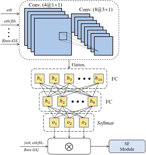
Figure 7. Network architecture of the feature attention module. $\otimes$ represents the Hadamard product, which performs element-wise multiplication between the generated feature weights and the input parameters.

In this equation, $w_{a_1}$ and $w_{a_2}$ represent the weights of the CNN layer, while $b$ denotes the bias value. The hyperbolic tangent function $\tanh (\cdot )$ is used for activation. These similarity weights are then applied to the input parameters to generate the weighted data ${\tilde{x}}^m=C_w(x^m,Y)x^m$.

2. Multi-Layer Perceptron Layer: Using ${\tilde{x}}^m$ as the input data for the multi-layer perceptron (MLP) layer, along with feedback information from the CNN layers $D_{t-1}$, the feature attention weights $e_t^m$ for the logging parameters toward the representation target are calculated as shown in Equation 3.

$e_t^m=v_t^m\tanh \left(D_{t-1}+u_t^m{\tilde{x}}_t^m+b_t^m\right)(3)$

Here, $v_t^m$, $u_t^m$, and $b_t^m$ represent the trained weights and biases of the perceptron layer.

3. Softmax Layer: The feature attention weights $e_t^m$ are normalized through the softmax layer to obtain the normalized feature attention weights $F_t^m$, as described in Equation 4.

$F_t^m=softmax\left(e_t^m\right)(4)$

4. Weighted Logging Data: Using the normalized feature attention weights, the input logging data $x_t^m$ is either enhanced or attenuated $(F_t^m{x}_t^m)$, depending on its linear correlation to the target, to generate the key logging features ${\tilde{x}}_t$ as input for the SF module, as defined in Equation 5.

${\tilde{x}}_t=\left(F_t^1{x}_t^1,F_t^2{x}_t^2,\dots ,F_t^m{x}_t^m\right)(5)$

The main goal of the Feature Attention Module is to dynamically adjust the weights of input features, enabling the model to focus on the most relevant features and thus improving classification accuracy. In the task of sedimentary micro-scale facies classification, the input data contains various types of features (such as thickness, Rmn-GS, etc.), and these features have different levels of importance across different micro-scale facies. Therefore, the model needs a mechanism to identify and emphasize those features that are most critical to the classification outcome.

Specifically, the Feature Attention Module calculates an “attention score” for each feature and assigns a weight to it, allowing the model to focus more on features with higher influence during training. During classification, some features may have a decisive impact on the result, while others may provide only supplementary information. Through the attention mechanism, the model can effectively distinguish the relative importance of these features, thereby achieving more precise classification.

3.3 Spatial feature extraction

Convolutional neural networks (CNNs) possess strong nonlinear fitting capabilities and the inherent advantage of weight sharing, which are instrumental in extracting spatial information from the nonlinear latent relationships between logging data and sedimentary micro-scale facies. These properties enhance model accuracy while significantly reducing computational costs. Building on these strengths, a spatial features (SF) module has been developed to capture the multi-scale spatial features of various logging parameters. This module is composed of three CNN layers: the first layer has 16 $1\times 1$ convolutional kernels, the second layer has 8 $1\times 1$ convolutional kernels, and the third layer has 16 $3\times 3$ convolutional kernels. Each layer’s structure incorporates operations such as input, convolution, activation, and pooling.

Key logging features serve as the input data for the SF module. Through processing, the module extracts spatial feature information, as described in Equation 6. The spatial information output from the first CNN layer is fed back to the FAtt module, while the output from the third CNN layer serves as the input for the Temporal Features (TF) module.

$D_{N,t}^i=R\left(w_{N,t}^i\otimes \left({\tilde{x}}^t\right)+b_{N,t}^i\right)(6)$

where $D_{N,t}^i$ represents the output value of the $N$-th neuron $(N\in [\mathrm{1,12}])$ in the $i$-th network layer at time $t$. Here, $i=\mathrm{1,2,3}$ refers to the specific network layer. The function $R(\cdot )$ denotes the ReLU activation function, while $w$ and $b$ correspond to the weights and biases of the CNN network, respectively. The symbol $\otimes$ signifies the convolution operation.

The Spatial Feature Extraction module uses Convolutional Neural Networks (CNN) to extract spatial features from the input data. Geological data often exhibits spatial structural characteristics, especially the sedimentary layers and geological features, which display distinct spatial distribution patterns. Therefore, effectively extracting spatial features from the data is crucial for improving the model’s classification accuracy.

CNN has significant advantages in extracting spatial features. It can automatically identify local spatial patterns in the input data and abstract high-level spatial features through convolution operations. In this model, CNN is responsible for handling spatial information in the geological data, such as the distribution of sedimentary layers, helping the model recognize spatial differences between different micro-scale facies. Specifically, the spatial feature extraction module uses multiple convolution and pooling operations to extract spatial features from the raw input data. Through iterative spatial feature learning, CNN is able to capture both local and global spatial patterns in the input data and pass these features to subsequent modules for deeper analysis and classification. In the case of severe horizontal and vertical heterogeneity in the river channel sand bodies in the study area, CNN can significantly enhance the model’s classification capability.

3.4 Temporal feature extraction

Logging data is typically acquired as a time-ordered sequence, where the information for each logging attribute at a given depth is not only influenced by subsequent depths but also closely related to preceding depths. To capture the temporal features of logging data within a certain depth range, a Temporal Features (TF) module has been constructed, consisting of four stacked LSTM layers. The network structure of the first layer in this module is shown in Figure 8. In the figure, $x_t$ represents the input data at time step $t$, $h_t$ represents the hidden state at time step $t$, and $C_t$ represents the cell state at time step $t$. The forget gate $f_t$ determines the information to be forgotten from the cell state at time step $t$, while the input gate $i_t$ determines the new information to be stored in the cell state at time step $t$. The candidate cell state ${\tilde{C}}_t$ is the new information generated at time step $t$, and the output gate $o_t$ determines the information to be output as the hidden state at time step $t$. The sigmoid activation function $\sigma$ is used to control the flow of information, $\otimes$ denotes the Hadamard product (element-wise multiplication) and $\oplus$ denotes element-wise addition, which is used to update the cell state $C_t$ by combining the outputs of the forget gate and the input gate.

Figure 8

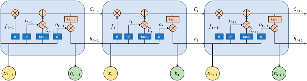
Figure 8. The architecture of LSTM units in temporal features module.

The spatial feature information output from the SF module is fed into the Temporal Features (TF) module. The process of extracting temporal features within a certain time range is described as follows:

1. Forget Gate: The input information $x_t^1=[D_{1,t}^3,D_{2,t}^3,\dots ,D_{N,t}^3]$ at time $t$ and the output information $h_{t-1}^1=[h_{1,t-1}^1,h_{2,t-1}^1,\dots ,h_{N,t-1}^1]$ from the previous moment are merged. The forget gate performs key feature extraction by calculating the feature extraction probability $f_t^1$ using Equation 7:

$f_t^1=1/\left(1+\exp \left[-\left(w_f^1{x}_t^1+u_f^1{h}_{t-1}^1+b_f^1\right)\right]\right)(7)$

where $w_f^1$ and $u_f^1$ are the weights of the forget gate, and $b_f^1$ is the bias. The superscripts indicate the LSTM layer number, ranging from 1 to 4.

2. Input Gate: The input gate extracts key parameter features from the current input data and the historical memory information from the previous moment. The feature extraction probability $i_t^1$ of the input gate is calculated using Equation 8:

$i_t^1=\frac{1}{1+\exp \left[-\left(w_i^1{x}_t^1+u_i^1{h}_{t-1}^1+b_i^1\right)\right]}(8)$

3. Temporary Feature Memory Cell: A temporary feature memory cell, ${\tilde{C}}_t^1$, is generated through the Tanh function, which integrates new logging parameter information into the memory cell, as expressed in Equation 9:

${\tilde{C}}_t^1=\frac{1-\exp \left[-2\left(w_c^1{x}_t^1+u_c^1{h}_t^1+b_c^1\right)\right]}{1+\exp \left[-2\left(w_c^1{x}_t^1+u_c^1{h}_t^1+b_c^1\right)\right]}(9)$

Temporary feature memory cell ${\widehat{C}}_{t-1}^1$, which is highly related to the target of sedimentary micro-scale facies identification, is determined by multiplying feature probability $f_t^1$ with the memory information of the previous moment $C_{t-1}^1$, represented as ${\widehat{C}}_{t-1}^1=f_t^1\times C_{t-1}^1$. The key feature memory information for the current moment, $C_{t-1}^1$, is established by weighting the temporary feature memories from the previous and current moments, represented as $C_t^1={\widehat{C}}_{t-1}^1+i_t^1\times {\tilde{C}}_t^1$.

4. Output Gate: The output gate processes the input data and historical memory information to calculate the feature extraction probability of the output gate, $O_t^1$, using Equation 10:

${\tilde{O}}_t^1=\frac{1}{1+\exp \left[-\left(w_0^1{x}_t+u_0^1{h}_{t-1}^1+b_0^1\right)\right]}(10)$

where $w_0^1$ and $u_0^1$ represent the weights, and $b_0^1$ is the bias of the output gate. The key parameter features for lithofacies classification are determined by weighting the current moment’s key feature memory information $C_t^1$ with the output gate’s feature extraction probability, as shown in Equation 11:

$h_t^1=O_t^1\times \frac{1-\exp \left(-2C_t^1\right)}{1+\exp \left(-2C_t^1\right)}(11)$

5. Classification: The output information from the TF module is input into the fully connected network and processed using the Softmax activation function to obtain the probabilities of sedimentary micro-scale facies categories, as expressed in Equation 12:

$P_k=\frac{\exp \left(w_k{h}_t^3+b_k\right)}{{\sum }_{k=1}^4\exp \left(w_k{h}_t^3+b_k\right)}(12)$

where $P_k$ denotes the probability of the $k$-th lithofacies category, while $w_k$ and $b_k$ represent the trained weights and biases of the $k$-th neuron in the fully connected network layer.

The Temporal Feature Extraction module uses Long Short-Term Memory (LSTM) networks to capture the temporal dependencies in the data. In sedimentary micro-scale facies classification tasks, especially with depth-related information, geological data often exhibits clear temporal dependencies — that is, as the depth increases, the features of the sedimentary micro-scale facies change. This depth dependency indicates that the differences between micro-scale facies are closely related to depth. Therefore, effectively capturing and modeling the temporal features in the data is crucial for improving the model’s classification accuracy.

LSTM has unique advantages in handling temporal data. It retains long-term dependency information through memory cells, making it particularly suitable for capturing long-term dependencies in depth changes or time series. In this model, LSTM handles the temporal dependencies in geological data, linking the features of each depth layer with those of adjacent layers. By using LSTM, the model can better understand the relationships between different depth layers, accurately handling the complex feature differences that arise with depth changes, and correctly classifying micro-scale facies with depth-dependent characteristics.

3.5 Evaluation metrics

To intuitively evaluate the sedimentary micro-scale facies identification performance of the model, this paper employs a confusion matrix to illustrate the prediction accuracy across different categories, as shown in Table 5. The confusion matrix compares the predicted categories with the actual categories, with each cell representing the number of instances where the model classified samples into specific categories.

Table 5

Table 5. Confusion matrix for evaluating model performance.

Accuracy is a commonly used evaluation metric. It is defined as the ratio of correctly predicted samples to the total number of samples, as shown in Equation 13.

$\text{Accuracy}=\frac{TP+TN}{TP+TN+FP+FN}(13)$

F1-score is another common evaluation metric for sedimentary micro-scale facies classification, as defined in Equation 14.

$\text{F}1-\text{score}=\mathrm{2}\times \frac{\mathrm{P}\mathrm{r}\mathrm{e}\mathrm{c}\mathrm{i}\mathrm{s}\mathrm{i}\mathrm{o}\mathrm{n}\times \mathrm{R}\mathrm{e}\mathrm{c}\mathrm{a}\mathrm{l}\mathrm{l}}{\mathrm{P}\mathrm{r}\mathrm{e}\mathrm{c}\mathrm{i}\mathrm{s}\mathrm{i}\mathrm{o}\mathrm{n}+\mathrm{R}\mathrm{e}\mathrm{c}\mathrm{a}\mathrm{l}\mathrm{l}}(14)$

where $\mathrm{P}\mathrm{r}\mathrm{e}\mathrm{c}\mathrm{i}\mathrm{s}\mathrm{i}\mathrm{o}\mathrm{n}=\frac{TP}{TP+FP}$ denotes precision, which measures the accuracy of identifying the kth sedimentary micro-scale facies class, and $\mathrm{R}\mathrm{e}\mathrm{c}\mathrm{a}\mathrm{l}\mathrm{l}=\frac{TP}{TP+FN}$ represents recall, which reflects the probability that samples belonging to the kth sedimentary micro-scale facies class are correctly identified. A higher recall indicates fewer misclassifications.

Precision and recall are often conflicting metrics, as improving one typically leads to a reduction in the other. F1-score balances precision and recall, providing a single metric that considers both. Consequently, this paper adopts both accuracy and F1-score as the evaluation metric for model construction.

4 Case study

4.1 Operating environment

In this study, all model training and testing code were executed on the Windows platform using the TensorFlow and Keras deep learning frameworks. To evaluate the performance of the FASTN model proposed in this paper, five additional models, Long Short-Term Memory (LSTM), Gated Recurrent Unit (GRU), Support Vector Machine (SVM), and Backpropagation Neural Network (BP) were developed for comparison. The input data and experimental settings for all models were kept consistent: We performed five-fold cross-validation for all models. In this approach, the entire dataset is divided into five equal-sized subsets. Each subset is used as a test set once, while the remaining four subsets are combined to form the training set. This process is repeated five times, ensuring that each subset is used as a test set exactly once. Consequently, in each fold, the training set size is 80% of the entire dataset, and the test set size is 20%. To prevent overfitting, Dropout techniques and the Adam optimizer were employed.

Network parameters for FASTN were iteratively tuned, achieving optimal performance with the following settings: an initial learning rate of $1\mathrm{e}-3$, Adam used as the optimizer, dropout set to 0.15, 100 iterations, and a batch size of 4. The loss function is set to cross-entropy. Due to the computational challenges associated with training the model, the hyperparameters were carefully selected to balance training efficiency and predictive accuracy. By employing five-fold cross-validation, the randomness associated with data partitioning is mitigated. This approach eliminates the need for a separate validation set, fully utilizes the dataset, and ensures the comprehensiveness and stability of model evaluation (Muscarella et al., 2014).

4.2 Comparative experiments and analysis

This experiment was conducted using the logging dataset constructed from 15 tightly spaced core wells and 51 main wells in the study area for training and testing. We conduct comparative experiments to evaluate the performance of the proposed FASTN model against several traditional and advanced neural network models, including LSTM, GRU, SVM, and BP, as shown in Table 6. The aim is to demonstrate the superiority of the FASTN model in terms of accuracy and efficiency for the subdivision of channel sand sedimentary micro-scale facies. The architectures and configurations of these baseline models are detailed below. The hyperparameters of these baseline models were carefully selected and manually tuned based on preliminary experiments to ensure that their performance was not underestimated. This approach ensures a fair comparison between different models.

Table 6

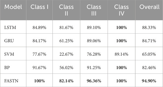
Table 6. Comparison of model performance. The optimal results are shown in bold.

Long Short-Term Memory (LSTM): We employ a three-layer unidirectional LSTM model. The input layer receives standardized data. The core of the model consists of three stacked LSTM layers, each with 16 hidden units, incorporating a 0.15 dropout rate to mitigate overfitting. The final LSTM output is passed through a fully connected layer, mapping to four classes, followed by a Softmax activation function to obtain class probabilities. The model is optimized using the Adam optimizer with a learning rate of $1\mathrm{e}-3$, and the loss function is set to cross-entropy. Training is conducted with a batch size of 4 for 100 epochs.

Gated Recurrent Unit (GRU): We employ a three-layer GRU model. The input layer receives standardized well-logging data, while the core network comprises three GRU layers, each with 16 hidden units and a 0.15 dropout rate to mitigate overfitting. The final GRU output is passed through a fully connected layer, mapping to four classes, followed by a Softmax activation function for probability distribution. The model is optimized using the Adam optimizer with a learning rate of $1\mathrm{e}-3$, and cross-entropy is used as the loss function. Training is conducted with a batch size of 4 for 100 epochs.

Support Vector Machine (SVM): The Support Vector Machine (SVM) we use applies the Radial Basis Function (RBF) kernel to classify the input standardized logging data. The input layer receives the standardized feature data. By choosing the RBF kernel, the model is able to capture complex nonlinear relationships in the data. To prevent overfitting, the model uses regularization parameters C = 1 and gamma = ‘scale’, where C controls the tolerance for errors, and gamma controls the complexity of the model.

Backpropagation Neural Network (BP): The BP neural network we use consists of three fully connected layers. The input layer receives standardized well log data. The network has three hidden layers, each with 16 neurons, and uses the ReLU activation function to enhance nonlinear representation capability. To prevent overfitting, a dropout rate of 0.15 is applied between the hidden layers. In the output layer, the data passes through a fully connected layer and produces a probability distribution over four categories, with a Softmax activation function for normalization. The network is optimized using the Adam optimizer with a learning rate of $1\mathrm{e}-3$, and the loss function is cross-entropy loss. The training process uses a batch size of 4 for iterations, with a total of 100 epochs.

The recognition accuracy of SVM for Class II (Channel Sand) is only 22.67%. This is due to the inherent limitations of SVM when dealing with non-linear and complex data. Particularly when faced with high-dimensional and noisy data, traditional SVM models are heavily affected. SVM relies on the internal structure of the sample data, and its parameter optimization is relatively complex. For geological data that exhibits significant complexity and heterogeneity, SVM fails to effectively capture the feature differences, leading to poor classification performance.

The performance of BP (Backpropagation Neural Network) in Class II is significantly weaker than that of the other three classes, with an accuracy of only 56.02%. BP is highly susceptible to initial weights, sensitive to data noise, and prone to falling into local optima. In Class II recognition, because of its relatively simple data processing approach, BP likely fails to effectively extract the complex relationships between the data.

GRU (Gated Recurrent Unit) achieves an accuracy of only 61.25% for Class II (Channel Sand). Although GRU can capture the depth-dependent changes in sedimentary micro-scale facies, it still struggles to correctly classify some categories with ambiguous boundaries. The relatively simple structure of GRU limits its ability to capture temporal and spatial features effectively, resulting in an inability to distinguish differences between similar features.

LSTM (Long Short-Term Memory) achieves an accuracy of 81.67% for Class II, which is an improvement over GRU. The model complexity of LSTM is higher than that of GRU, and it is more reliant on data, requiring effective selection and weighting of the data.

By introducing a feature attention mechanism, FASTN dynamically adjusts the weights of input features, allowing the model to focus more on the most relevant geological features for the task. This mechanism significantly improves recognition accuracy, particularly in complex sedimentary micro-scale facies classification tasks. For categories with distinct geological features, such as Class I (Incised Zone) and Class IV (Abandoned Channel), the FASTN model improves classification accuracy by enhancing the weights of the relevant features, achieving a perfect accuracy of 100% for these two categories. Additionally, FASTN also achieves an accuracy of 82.14% for Class II and 96.36% for Class III, with an overall accuracy of 94.9%, which is the best model among all.

FASTN combines a spatial module and a temporal module, integrating Convolutional Neural Networks (CNN) and Long Short-Term Memory (LSTM) networks to simultaneously extract spatial and temporal features. The CNN is primarily used to extract spatial information from logging data, while LSTM is adept at capturing temporal dependencies. By using LSTM to capture temporal information and combining it with CNN for spatial feature processing, especially in cases of significant geological changes and deep information impacts, FASTN can more accurately delineate micro-scale facies, compensating for the inability of traditional models to handle the complex relationship between depth and temporal sequences effectively.

4.3 Ablation study

To further verify the impact of each module on the performance of channel sand sedimentary micro-scale facies identification, this study conducted ablation experiments. The ablation experiments involved gradually removing certain key components of the model to assess each module’s contribution to the overall performance of the model. This approach allows for a clear understanding of the role that each module plays in enhancing model performance and provides a basis for future model optimization and improvement. In the ablation experiments, the model’s performance under different module configurations was tested, demonstrating the effectiveness of each module and its contribution to improving model accuracy. Table 7 presents the ablation results for each sedimentary micro-scale facies class, along with the overall identification performance of each model.

Table 7

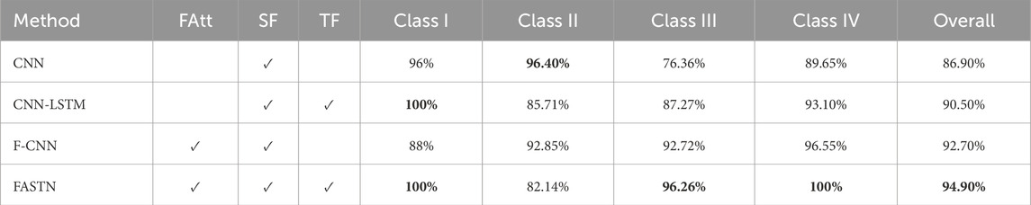
Table 7. Results of ablation study. In the table, “$✓$” denotes the model contains this module. The optimal results are shown in bold.

Figure 9 shows the parameter curves of the test set and the distribution of channel sand sedimentary micro-scale facies identification results across different models in the ablation study compared to the actual lithofacies.

Figure 9

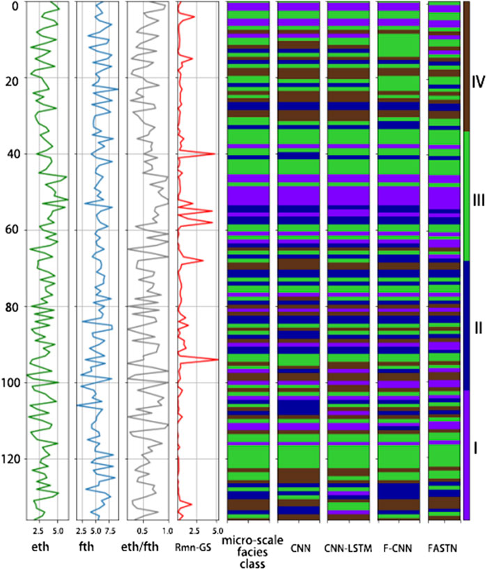
Figure 9. Test set logging curves and sedimentary micro-scale facies identification results of different models.

From Figure 9, it is evident that the CNN model exhibits noticeable underfitting in lithofacies classification. For instance, at sample points 11, 20, 25, 31, 78, 96, 124, 125, and 135, the model incorrectly classifies the third type of channel facies as the fourth type. At sample point 95, the fourth type of channel facies is misclassified as the third type; at sample point 97, the first type is misclassified as the second type; and at sample points 40, 87, and 106, the third type is misjudged as the second type. Significant misclassification issues are observed between the third and fourth types of channel sand sedimentary micro-scale facies. According to the classification standards for the third and fourth types of channel sands, this indicates that the CNN model struggles with feature extraction for the parameter Rmn-GS.

The CNN-LSTM model, with its Temporal Features (TF) module, improves the extraction of temporal features, leading to a notable reduction in misclassification of channel sand facies samples. For example, at sample points 20, 25, 31, 96, 101, 124, and 135, the third type of channel sand sedimentary micro-scale facies is mistakenly identified as the fourth type. At points 55, 108, 129, and 134, the second type is misjudged as the first type. The TF module enhances the ability of the model to capture temporal features by leveraging the cumulative effect of logging parameters over time, thereby mitigating boundary ambiguity issues introduced by manual classification standards.

The F-CNN model demonstrates enhanced discriminative capability for the third and fourth types of channel sand sedimentary micro-scale facies. Misclassifications are limited to a few sample points, such as where the third type is misclassified as the first type (sample point 9), the fourth type (sample point 12), and where the second type (sample point 13) is misclassified as the third type. By applying attention to both spatial and temporal features, the F-CNN model better differentiates between similar classes, significantly reducing misclassifications between the third and fourth types of channel sand sedimentary microfacies. This highlights the crucial role of feature attention in improving classification performance, especially in cases where sedimentary facies exhibit subtle differences that are challenging for traditional models to distinguish. The inclusion of the attention module enables the model to assign appropriate weights based on the relevance of input parameters to the target, allowing it to focus on critical logging parameters like Rmn-GS for more accurate delineation of sedimentary microfacies characteristics.

The FASTN model exhibits the fewest misclassified samples among the tested models. Misclassifications occur at sample points 13, 64, 67, and 91, where the second type of channel facies is misidentified as the first type, and at sample point 101, where the third type is also misclassified as the first type. Additionally, one instance is observed where the third type of channel sand sedimentary micro-scale facies (sample point 68) is misclassified as the second type. Compared to the F-CNN model, the FASTN model, which combines the feature attention mechanism with both CNN and LSTM modules, shows significant improvements in temporal feature extraction and precision in subdividing the channel sand sedimentary micro-scale facies. The enhanced spatial and temporal feature extraction, along with a focus on the most important features, enables the FASTN model to achieve superior classification accuracy. The misclassification rates are notably reduced across all sample points, and the boundary between the third and fourth types of microfacies is more clearly defined. This demonstrates the effectiveness of the FASTN model in addressing the challenges faced by previous models and offering a more robust and accurate solution for sedimentary microfacies classification.

Figure 10 shows the confusion matrices of different models, which presents the channel sand sedimentary micro-scale facies identification results for different models using three input parameters. The horizontal and vertical coordinates 1-4 represent class I-IV of channel sand sedimentary micro-scale facies. The CNN model achieves an overall accuracy of 86.9%. It correctly identifies 24 instances of the first type of channel sand sedimentary micro-scale facies, with 1 misclassified as the second type; correctly classifies 27 instances of the second type, with 1 misclassified as the third type; accurately recognizes 42 instances of the third type, but 3 and 10 are misclassified as the second and fourth types, respectively; and correctly identifies 26 instances of the fourth type, with 2 and 1 misclassified as the second and third types, respectively. Notably, the CNN model demonstrates poor identification performance for the third type of channel facies, with an F1-score of only 84.9%.

Figure 10

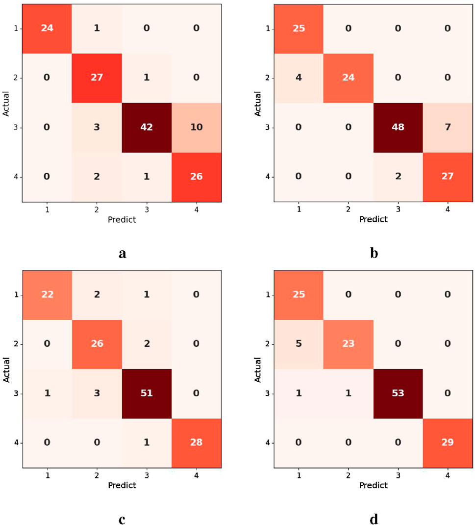
Figure 10. Results of channel sand sedimentary micro-scale facies identification of different models. (a) CNN, (b) CNN-LSTM, (c) F-CNN, (d) FASTN.

Compared to the CNN model, the CNN-LSTM model demonstrates an improvement of 3.6% in identification accuracy, correctly identifying 25, 24, 48, and 27 instances of the four channel sand sedimentary micro-scale facies, respectively. The misclassification rate for the third and fourth types of channel sand sedimentary micro-scale facies has significantly decreased, with the best identification performance observed for the first type. This highlights the advantage of the model in extracting key spatio-temporal features.

Building on the CNN model, the incorporation of the feature attention module for weighting input parameters allows the F-CNN model to achieve a sedimentary micro-scale facies identification accuracy of 92.7%, with 10 instances misclassified into other categories. The FASTN model further improves the overall identification accuracy to 94.9%, achieving 100% accuracy for the first and fourth types of sedimentary micro-scale facies, and FASTN performs well on the third type, with an F1-score of 98.2%. Only a small number of instances (7) are misclassified, and the model exhibits more precise boundary delineation between the third and fourth types. This enables accurate and intelligent identification of channel sand sedimentary micro-scale facies, providing essential data support for further clarifying the interconnection between injection and production well groups.

4.4 Universality analysis

Using the same network structure and parameters, this study tested another dataset from a different work area. The same logging parameters were selected, with 190 sample sets designated as the test set (20%) to achieve intelligent identification of channel sand sedimentary micro-scale facies.

Figure 11 presents the identification results of the proposed method, achieving an F1-score of 94.70%. Five instances of the first type of sedimentary micro-scale facies were misclassified as the second type, while the boundaries between the third and fourth types of sedimentary micro-scale facies were clearly delineated, with only 2 misclassifications. Additionally, the identification accuracy for the fourth type of sedimentary micro-scale facies reached 100%. These experimental results demonstrate that the proposed method is applicable for channel sand sedimentary micro-scale facies identification across different work areas.

Figure 11

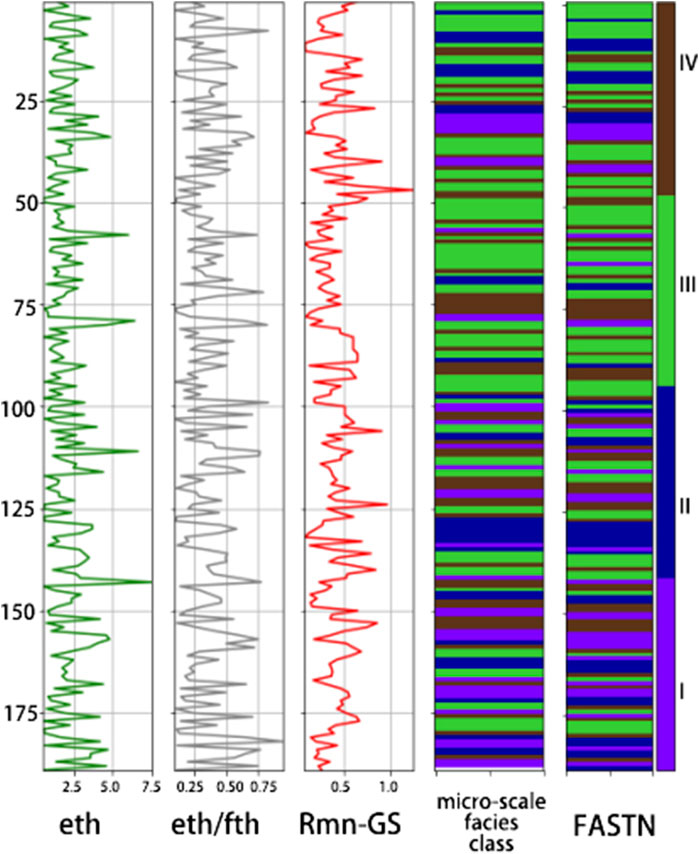
Figure 11. Results of channel sand sedimentary micro-scale facies identification across another work area.

5 Conclusion

This paper proposes a deep learning-based method for intelligent identification of channel sand sedimentary micro-scale facies, focusing on extracting key logging parameter features to achieve high-precision reservoir subdivision. The main contributions are as follows:

1. The study selects eth, eth/fth, and Rmn-GS as key feature parameters to establish a classification standard for channel sand sedimentary micro-scale facies, providing a refined characterization method for reservoir connectivity between injection and production wells.

2. The proposed FASTN model incorporates an LSTM network, effectively handling depth and temporal relationships in logging curves. The feature attention module dynamically assigns weights to parameters, enabling the model to focus on more critical features, achieving an accuracy improvement of 8% compared to traditional CNN models.

3. FASTN effectively handles nonlinear relationships in data, demonstrating strong generalization capability and providing a novel approach for intelligent sedimentary micro-scale facies identification. Compared to traditional manual methods, it significantly improves work efficiency and identification accuracy, achieving a subdivision accuracy of over 94%. The method has been applied in the Daqing Oilfield, offering valuable guidance for reservoir development.

Data availability statement

The raw data supporting the conclusions of this article will be made available by the authors, without undue reservation.

Author contributions

RZ: Conceptualization, Investigation, Methodology, Software, Validation, Visualization, Writing–original draft, Writing–review and editing. LZ: Conceptualization, Data curation, Formal Analysis, Methodology, Project administration, Resources, Software, Supervision, Visualization, Writing–original draft, Writing–review and editing. CF: Funding acquisition, Writing–review and editing. XZ: Data curation, Formal Analysis, Funding acquisition, Investigation, Project administration, Resources, Supervision, Validation, Writing–review and editing.

Funding

The author(s) declare that financial support was received for the research, authorship, and/or publication of this article. The Natural Science Foundation of Hebei Province, Hebei, China (D2022107001). The Key of Program of the National Natural Science Foundation of China under Grants (61933007, 61873058, and 42002138), China. The Basic Research Funding for Universities in Heilongjiang Province (1501202201), Heilongjiang, China.

Conflict of interest

Author CF was employed by China National Logging Corporation.

The remaining authors declare that the research was conducted in the absence of any commercial or financial relationships that could be construed as a potential conflict of interest.

The reviewer XW declared a shared affiliation with the authors LZ, XZ to the handling editor at time of review.

Generative AI statement

The author(s) declare that no Generative AI was used in the creation of this manuscript.

Publisher’s note

All claims expressed in this article are solely those of the authors and do not necessarily represent those of their affiliated organizations, or those of the publisher, the editors and the reviewers. Any product that may be evaluated in this article, or claim that may be made by its manufacturer, is not guaranteed or endorsed by the publisher.

References

Aslam, M., Lee, J.-M., Altaha, M. R., Lee, S.-J., and Hong, S. (2020). Ae-lstm based deep learning model for degradation rate influenced energy estimation of a pv system. Energies 13, 4373. doi:10.3390/en13174373

CrossRef Full Text | Google Scholar

Cao, D., Chen, Y., Chen, J., Zhang, H., and Yuan, Z. (2021). An improved algorithm for the maximal information coefficient and its application. R. Soc. open Sci. 8, 201424. doi:10.1098/rsos.201424

PubMed Abstract | CrossRef Full Text | Google Scholar

Chen, L., Lin, W., Chen, P., Jiang, S., Liu, L., and Hu, H. (2021). Porosity prediction from well logs using back propagation neural network optimized by genetic algorithm in one heterogeneous oil reservoirs of ordos basin, China. J. Earth Sci. 32, 828–838. doi:10.1007/s12583-020-1396-5

CrossRef Full Text | Google Scholar

Cherana, A., Aliouane, L., Doghmane, M. Z., Ouadfeul, S.-A., and Nabawy, B. S. (2022). Lithofacies discrimination of the ordovician unconventional gas-bearing tight sandstone reservoirs using a subtractive fuzzy clustering algorithm applied on the well log data: illizi basin, the algerian sahara. J. Afr. Earth Sci. 196, 104732. doi:10.1016/j.jafrearsci.2022.104732

CrossRef Full Text | Google Scholar

Choi, E., Cho, S., and Kim, D. K. (2020). Power demand forecasting using long short-term memory (lstm) deep-learning model for monitoring energy sustainability. Sustainability 12, 1109. doi:10.3390/su12031109

CrossRef Full Text | Google Scholar

Cowan, N. (2001). The magical number 4 in short-term memory: a reconsideration of mental storage capacity. Behav. brain Sci. 24, 87–114. doi:10.1017/s0140525x01003922

PubMed Abstract | CrossRef Full Text | Google Scholar

de Lima, R. P., Duarte, D., Nicholson, C., Slatt, R., and Marfurt, K. J. (2020). Petrographic microfacies classification with deep convolutional neural networks. Comput. and geosciences 142, 104481. doi:10.1016/j.cageo.2020.104481

CrossRef Full Text | Google Scholar

dos Santos, D. T., Roisenberg, M., and dos Santos Nascimento, M. (2021). Deep recurrent neural networks approach to sedimentary facies classification using well logs. IEEE Geoscience Remote Sens. Lett. 19, 1–5. doi:10.1109/lgrs.2021.3053383

CrossRef Full Text | Google Scholar

Feng, R. (2024). “Gated recurrent units for lithofacies classification based on seismic inversion,” in Artificial intelligent approaches in Petroleum geosciences (Springer), 97–113.

Google Scholar

Feng, Y., Gong, X., Xu, Y., Xie, Z., Cai, H., and Lv, X. (2019). Lithology recognition based on fresh rock images and twins convolution neural network. Geogr. Geogr. Inf. Sci. 35, 89–94. doi:10.3969/j.issn.1672-0504.2019.05.015

CrossRef Full Text | Google Scholar

Guo, A. J., and Zhu, F. (2019). A conn-based spatial feature fusion algorithm for hyperspectral imagery classification. IEEE Trans. Geoscience Remote Sens. 57, 7170–7181. doi:10.1109/tgrs.2019.2911993

CrossRef Full Text | Google Scholar

Hou, X., Zhu, Y., Chen, S., Wang, Y., and Liu, Y. (2020). Investigation on pore structure and multifractal of tight sandstone reservoirs in coal bearing strata using lf-nmr measurements. J. Petroleum Sci. Eng. 187, 106757. doi:10.1016/j.petrol.2019.106757

CrossRef Full Text | Google Scholar

Imamverdiyev, Y., and Sukhostat, L. (2019). Lithological facies classification using deep convolutional neural network. J. Petroleum Sci. Eng. 174, 216–228. doi:10.1016/j.petrol.2018.11.023

CrossRef Full Text | Google Scholar

Kaakinen, A., Salonen, V.-P., Kubischta, F., Eskola, K. O., and Oinonen, M. (2009). Weichselian glacial stage in murchisonfjorden, nordaustlandet, svalbard. Boreas 38, 718–729. doi:10.1111/j.1502-3885.2009.00092.x

CrossRef Full Text | Google Scholar

Khan, S. Q., and Kirmani, F. U. D. (2024). Applicability of deep neural networks for lithofacies classification from conventional well logs: an integrated approach. Petroleum Res. 9, 393–408. doi:10.1016/j.ptlrs.2024.01.011

CrossRef Full Text | Google Scholar

Li, W. B., Yu, Y. L., Wang, J. Q., Bai, Y., and Wang, X. (2013). Application of self-organizing neural network method in logging sedimentary microfacies identification. Adv. Mater. Res. 616, 38–42. doi:10.4028/www.scientific.net/amr.616-618.38

CrossRef Full Text | Google Scholar

Li, Y., Wang, H., Wang, M., Lian, P., Duan, T., and Ji, B. (2017). Automatic identification of carbonate sedimentary facies based on PCA and KNN using logs. Well Logging Technol. 41, 57–41. doi:10.16489/j.issn.1004-1338.2017.01.010

CrossRef Full Text | Google Scholar

Liu, X.-Y., Zhou, L., Chen, X.-H., and Li, J.-Y. (2020). Lithofacies identification using support vector machine based on local deep multi-kernel learning. Petroleum Sci. 17, 954–966. doi:10.1007/s12182-020-00474-6

CrossRef Full Text | Google Scholar

Liu, Y., Hu, M., Zhang, S., Zhang, J., Gao, D., and Xiao, C. (2022). Characteristics and impacts on favorable reservoirs of carbonate ramp microfacies: a case study of the Middle—lower Ordovician in Gucheng area, Tarim Basin, NW China. Petroleum Explor. Dev. 49, 107–120. doi:10.1016/s1876-3804(22)60008-9

CrossRef Full Text | Google Scholar

Luo, Z. R., Zhou, Y., Li, Y. X., Guo, L., Tuo, J. J., and Xia, X. L. (2022). Intelligent identification of sedimentary microfacies based on DMC-BiLSTM. Geophys. Prospect. Petroleum 61, 253–261. doi:10.3969/j.issn.1000-1441.2022.02.007

CrossRef Full Text | Google Scholar

Muscarella, R., Galante, P. J., Soley-Guardia, M., Boria, R. A., Kass, J. M., Uriarte, M., et al. (2014). Enm eval: an r package for conducting spatially independent evaluations and estimating optimal model complexity for maxent ecological niche models. Methods Ecol. Evol. 5, 1198–1205. doi:10.1111/2041-210x.12261

CrossRef Full Text | Google Scholar

Peng, Y., and Guo, S. (2023). Lithofacies analysis and paleosedimentary evolution of taiyuan formation in southern north China basin. J. Petroleum Sci. Eng. 220, 111127. doi:10.1016/j.petrol.2022.111127

CrossRef Full Text | Google Scholar

Shengli, L., Xinghe, Y., and Jianli, J. (2016). Sedimentary microfacies and porosity modeling of deep-water sandy debris flows by combining sedimentary patterns with seismic data: an example from unit i of gas field a, south China sea. Acta Geol. Sinica-English Ed. 90, 182–194. doi:10.1111/1755-6724.12650

CrossRef Full Text | Google Scholar

Shu, N., Wang, X., Su, C., Song, L., Niu, X., and Li, Q. (2017). Stepped and detailed seismic prediction of shallow-thin reservoirs in chunfeng oilfield of junggar basin, nw China. Petroleum Explor. Dev. 44, 595–602. doi:10.1016/s1876-3804(17)30068-x

CrossRef Full Text | Google Scholar

Song, C., Lu, W., Wang, Y., Jin, S., Tang, J., and Chen, L. (2022). Reservoir prediction based on closed-loop cnn and virtual well-logging labels. IEEE Trans. Geoscience Remote Sens. 60, 1–12. doi:10.1109/tgrs.2022.3205301

CrossRef Full Text | Google Scholar

Song, L. (2023). Research on the time-varying law of reservoir physical properties and the potential tapping method of water flooding chemical flooding adjustment in ultra-high water cut oil fields. Phd thesis, Northeast Univ. Petroleum. doi:10.26995/d.cnki.gdqsc.2023.000005

CrossRef Full Text | Google Scholar

Tang, C. (2023). “Identification of sedimentary microfacies based on genetic bp algorithm and image processing,” in 2023 international conference on applied intelligence and sustainable computing ICAISC (IEEE), 1–6.

CrossRef Full Text | Google Scholar

Tian, M., and Verma, S. (2022). “Recurrent neural network: application in facies classification,” in Advances in subsurface data analytics (Elsevier), 65–94.

CrossRef Full Text | Google Scholar

Wang, D., Peng, J., Yu, Q., Chen, Y., and Yu, H. (2019). Support vector machine algorithm for automatically identifying depositional microfacies using well logs. Sustainability 11, 1919. doi:10.3390/su11071919

CrossRef Full Text | Google Scholar

Yang, C., Jiang, Y., Song, B., Wang, G., and Zhang, X. (2022). Recognition technology integrating logging and seismic data for thin sand reservoir in narrow channel and its application: taking the agl area in western daqing placanticline as an example. Oil Geophys. Prospect. 57, 159–167. doi:10.13810/j.cnki.issn.1000-7210.2022.01.017

CrossRef Full Text | Google Scholar

Yang, H., Liu, W., Shan, X., and Yang, L. (2005). Sedimentary micro-facies distinguishing marks of delta-front of the west slope zone in southern Songliao basin and its application. Glob. Geol. 24, 43–47. doi:10.3969/j.issn.1004-5589.2005.01.007

CrossRef Full Text | Google Scholar

Zeng, L., Ren, W., Shan, L., and Huo, F. (2022). Well logging prediction and uncertainty analysis based on recurrent neural network with attention mechanism and Bayesian theory. J. Petroleum Sci. Eng. 208, 109458. doi:10.1016/j.petrol.2021.109458

CrossRef Full Text | Google Scholar

Zhang, H., Yang, X., Chen, Z., Zhao, H., Zhou, W., Huang, Z., et al. (2022a). A log data reconstruction method based on enhanced bidirectional long short-term memory neural network. Prog. Geophys. 37, 1214–1222. doi:10.6038/pg2022FF0194

CrossRef Full Text | Google Scholar

Zhang, K., Lin, N., Tian, G., Yang, J., Wang, D., and Jin, Z. (2022b). Unsupervised-learning based self-organizing neural network using multi-component seismic data: application to xujiahe tight-sand gas reservoir in China. J. Petroleum Sci. Eng. 209, 109964. doi:10.1016/j.petrol.2021.109964

CrossRef Full Text | Google Scholar

Zhang, Y.-c. (2013). Quantitative identification of sedimentary microfacies of fuyu oil layer in sanzhao depression. J. Oil Gas Technol. 35, 11–14. doi:10.3969/j.issn.1000-9752.2013.01.003

CrossRef Full Text | Google Scholar

Zhu, L., Li, H., Yang, Z., Li, C., and Ao, Y. (2018). Intelligent logging lithological interpretation with convolution neural networks. Petrophysics 59, 799–810. doi:10.30632/pjv59n6-2018a5

CrossRef Full Text | Google Scholar