Machine learning approach for prediction of safe mud window based on geochemical drilling log data

Background: Accurate prediction of the safe mud window (SMW) is critical for drilling operations to prevent costly risks such as blowouts, mud loss, and wellbore instability. Traditional geomechanical methods for SMW determination face challenges in handling complex, nonlinear relationships within drilling datasets.

Purpose: This study aims to develop robust machine learning (ML) models to predict two key SMW parameters—Mud Pressure below shear failure (MWsf) and tensile failure (MWtf)—using geochemical drilling log data from Middle Eastern carbonate reservoirs.

Methods: Hybrid ML models combining Least Squares Support Vector Machine (LSSVM) and Multilayer Perceptron (MLP) with optimization algorithms (Gray Wolf Optimization, GWO; Grasshopper Optimization Algorithm, GOA) were trained on 2,820 data points from three wells. Input variables included drilling time, caliper, weight on bit, flow rate, and rheological properties. Model performance was evaluated using RMSE, R², and cross-validation.

Results: The LSSVM-GWO model outperformed others, achieving RMSE values of 58.01 (MWsf) and 95.42 (MWtf) with R² > 0.99. Flow speed, rotor solids, and fan readings strongly influenced MWsf, while WOB, gel strengths, and flow rate impacted MWtf. Generalization testing on a third well confirmed robustness (RMSE: 50.26 for MWsf, 70.89 for MWtf).

Conclusion: The LSSVM-GWO framework provides a reliable, data-driven solution for SMW prediction, enabling safer and more efficient drilling operations. This approach reduces operational risks and highlights the potential of hybrid ML models in reservoir management.

1 Introduction

The concept of a safe mud window (SMW) is of utmost importance in the drilling industry, as it defines a range of mud weights that are safe for drilling operations (Li et al., 2016). Ensuring that mud weight is within this range is essential to avoid accidents, maintain efficient drilling, and prevent damage to the formation of the wellbore walls (Fu et al., 2022). Reservoir geomechanics is an important science in developing and optimizing drilling paths, reservoir planning, determination of reservoir pressure, and characterization of rock and reservoir properties (Abdelghany et al., 2021). One of its subsets is drilling pressure control, which is directly affected by pore pressure (PP) and fracture pressure (FP) (McWhorter et al., 2021). The determination of SMW is closely linked to PP and FP and plays a key role in drilling cost, mud loss, drilling fractures, in situ stress, drilling time, blowout, and casing collapse (CC) (Gowida et al., 2022). To determine SMW, it is important to establish the safe window, which is the distance between PP and FP and represents the safe point of SMW (Al-Nutaifi, 2019; Jafarizadeh et al., 2022)—exceeding FP results in mud loss, while pressure lower than PP leads to blow out. Hence, determining SMW is a vital factor in drilling operations that can greatly enhance drilling efficiency (Al-Nutaifi, 2019). Reecently many ML and DL techniques are come to solve many problem in different fields like; the inndustry, medicine, etc (Ghorbani et al., 2022; Ghorbani et al., 2023a; Ghorbani et al., 2023b; Lu et al., 2024). Different methods, including geomechanical and artificial intelligence methods (e.g., Bayesian Optimization, genetic algorithms), have been utilized by researchers to determine SMW, though their comparative efficacy in this context remains understudied.

Maleki et al. (2014) conducted a study to investigate the accuracy of three different failure criterion methods - Hoek-Brown, Mohr-Coulomb, and Mogi-Coulomb in predicting the SMW in two wells located in Iran and one well in Australia. The Mogi-Coulomb method showed higher accuracy in predicting failure than the other two methods, which could be attributed to considering intermediate stress in this method. This study provided valuable insights into selecting appropriate failure criterion methods for predicting SMW, which ensures wellbore stability in the oil industry (Maleki et al., 2014). Aslannezhad et al. (2016) investigated the estimation of well stability and SMW in Iran using the Mohr-Coulomb and Mogi-Coulomb failure criterion methods. They utilized well slope and azimuth changes to determine the lower and upper limits of mud pressure and well stability. Their study showed that both methods performed well in estimating well resistance and SMW, with the most stable drilling condition and highest SMW observed at a well slope of 30 and azimuth of 90 and 270. This study provided useful information for optimizing drilling operations and minimizing drilling-related issues (Aslannezhad et al., 2016). Zahiri et al. (2019) utilized the support vector machine with radial basis function (SVM-RBF) algorithm to calculate SMW based on data from three wells in Iran. They showed that this method is highly accurate in predicting SMW, with a coefficient of determination of 0.9329 and mean squared error (MSE) of 4.36. The authors emphasized using diverse and abundant data to improve the model’s accuracy. This study highlighted the potential of machine learning algorithms in predicting SMW, which can significantly improve drilling operations (Zahiri et al., 2019). Tewari (2019) compared the performance of several algorithms - artificial neural network (ANN), support vector regression (SVR), and random forest (RF) - in predicting SMW in a well located in the Norwegian Sea. The random forest algorithm performed best, with the highest R² of 0.9990 and the lowest root mean squared error (RMSE) of 0.0079. This study demonstrated the effectiveness of machine learning algorithms in predicting MW, which can help optimize drilling operations and reduce associated costs (Tewari, 2019). Phan et al. (2020) conducted a study to estimate time-dependent SMW using various methods, including decision tree (DT), linear regression (LR), RF, ANN, and extra trees (ET). They showed that the trained neural network had the highest accuracy in predicting SMW, with an R² of 0.998 and MSE of 0.043. The authors suggested that this method can be used to predict SMW accurately, which is critical in ensuring the safety and stability of the drilling operation (Phan et al., 2020). Gowida et al. (2022) utilized artificial neural network methods to predict SMW in the Middle East using various petrophysical data, including sonic data, formation bulk density, neutron log, gamma ray log, and caliper reports, obtained from experiments and drilling operations. The proposed model showed a high accuracy of more than 92% and a mean absolute percentage error (MAPE) of 0.53% in predicting SMW, highlighting its cost-effectiveness and potential for use in multiple wells. This study provided valuable insights into using artificial neural networks to predict SMW and improve drilling operations (Gowida et al., 2022). Reports related to the history of research in the field of SMW prediction are reported in Table 1.

Table 1

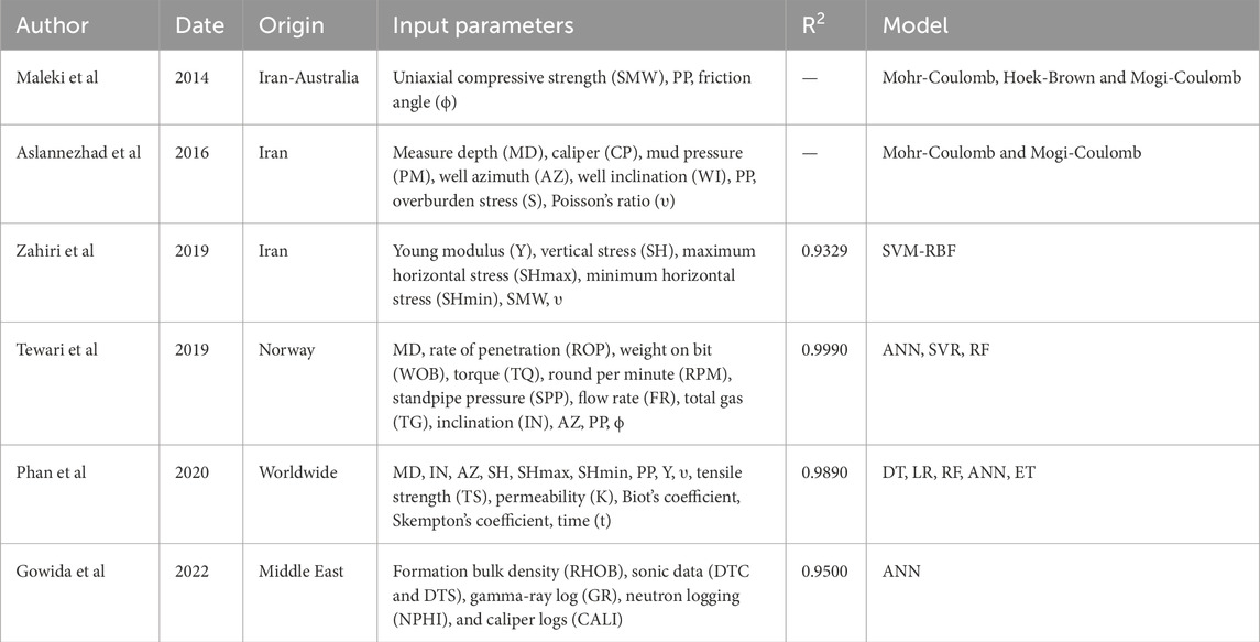
Table 1. Displays records concerning the historical background of research carried out in SMW prediction.

While existing studies demonstrate the utility of machine learning in SMW prediction, this study advances the field by integrating optimization algorithms (GWO/GOA) with LSSVM/MLP to address critical limitations. For instance, Zahiri et al. (2019) achieved an R² of 0.9329 using SVM-RBF, whereas Tewari (2019) reported R² = 0.9990 with RF. However, these methods often struggle with noise, nonlinearity, or generalization across diverse datasets. The proposed LSSVM-GWO hybrid achieves comparable or superior accuracy (R² > 0.99 for both MWsf and MWtf) while explicitly addressing overfitting via k-fold validation and optimizing hyperparameters through GWO. Unlike ANN-based approaches (e.g., Gowida et al., 2022: R² = 0.95), LSSVM-GWO requires fewer computational resources and handles small datasets more effectively. However, the dependency on parameter tuning via metaheuristics and the need for geochemical-specific training data remain limitations relative to simpler empirical models.

To detect SMW based on the prediction of MWsf and MWtf, this study utilized a variety of input parameters including drilling time (t), caliper (cP), weight on bit (WOB), flow rate (Q), retort solid (RS), fan 600/fan 300 (F600/F300), gel10min/gel10s (G10min/G10s), pump discharge pressure (Pw), and rotations per minute (RPM). Different machine-learning techniques were combined to achieve this goal, specifically LSSVM-GWO, MLP-GWO, LSSVM-GOA, and MLP-GOA. The dataset used for analysis consisted of 2,820 data points obtained from three wells (V1, V2, and V3) located in a carbonate oil field in the Middle East. Statistical evaluation of the models indicated that the LSSVM-GWO method outperformed the other techniques in predicting SMW. In the oil industry, accurate prediction of SMW is important to mitigate operational risks such as flow loss and blowouts. Precise SMW prediction helps optimize the mud window and prevents costly errors. This study’s utilization of machine learning techniques presents a promising approach to SMW prediction, as it allows for simultaneous analysis of multiple input parameters. This facilitates the identification of correlations between these parameters and enhances the accuracy of predictions. While prior studies have demonstrated the efficacy of individual ML algorithms (e.g., SVM-RBF, RF) in SMW prediction, this work introduces a hybrid approach combining LSSVM with metaheuristic optimizers (GWO/GOA). Unlike conventional geomechanical models (e.g., Mohr-Coulomb), which rely on deterministic relationships and often overlook nonlinear interactions, our method leverages ML to capture complex patterns in geochemical and operational data. Furthermore, the integration of GWO optimizes hyperparameters (e.g., regularization, kernel width) to enhance generalization, addressing limitations such as overfitting in RF and computational inefficiency in ANN.

2 Materials and methods

In order to visually represent the methodologies and procedures outlined in this research paper, we utilize the flowchart presented in Figure 1. The flowchart is a graphical depiction of the sequential steps involved in the analysis process. Initially, data is collected from three distinct wells (V1, V2, and V3) located within an oil field in the Middle East. Following data collection, a normalization process is employed (Equation 1), as detailed in the flowchart. The construction of artificial intelligence hybrid models, namely LSSVM-GWO, MLP-GWO, LSSVM-GOA, and MLP-GOA, is then undertaken utilizing the information obtained from wells V1 and V2. The primary objective of these models is to predict two significant parameters, MWsf and MWtf, ultimately providing a forecast for SMW. To ensure the integrity of the subsequent data analysis, the collected data from the two wells is divided into three subsets: a training set, a testing set, and a validation set. Employing the k-fold method, a technique designed to prevent overfitting further safeguards the accuracy and reliability of the analysis. Statistical error analysis is subsequently conducted to assess the results’ quality and effectiveness. Once the most optimal algorithm, LSSVM-GWO, is identified, the data acquired from well V3 is incorporated to expand and enhance the algorithm’s generalizability. The extended algorithm is then thoroughly evaluated to determine its efficacy and performance.

Figure 1

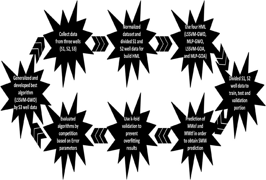
Figure 1. Flowchart diagram for prediction of the SMW.

Prior to applying for the ML models, the dataset underwent min-max normalization to scale input features within the range [0, 1]. This preprocessing step ensures uniform contribution of variables to the model, calculated as (Equation 1):

$x_{norm}=\frac{x-x_{\mathit{min}}}{x_{\mathit{max}}-x_{\mathit{min}}}(1)$

where x_min and x_max are the minimum and maximum values of each feature.

2.1 Least squares support vector machine (LSSVM)

One of the most effective methods based on statistical models is the LSSVM method. LSSVM is an improved version of the Support Vector Machine (SVM) method (Han et al., 2019). The SVM method traditionally requires significant effort and extensive calculations to solve problems (Lin et al., 2011). However, introducing LSSVM has facilitated the resolution of complex problems and achieving acceptable results. Consequently, researchers now prefer using the new LSSVM method instead of the classic SVM method to address challenging issues and problems. LSSVM establishes a suitable relationship between input and output parameters (Zhang and Zhang, 2016). The input parameters determine the collection points required to achieve the desired output. The relationship between the input and output parameters is expressed by Equation 2.

$Minimize=\frac{1}{2}{\omega }^T\omega +\frac{\gamma }{2}{\displaystyle \sum _{k=1}^l}{e}_k^2,y_k\left[{\omega }^T\phi \left(x_k\right)+b\right]=1-e_k,k=1,\dots ,N(2)$

The regularization parameter, γ, plays an important role in determining the balance between minimizing fitting errors and achieving smoothness. In addition, e_k represents the error variable. The optimization problem presented in Equation 1 is solved using Lagrange multipliers, and its solution is provided as follows (Equation 3):

$y\left(x\right)=sign\left[{\displaystyle \sum _{k=1}^N}{\alpha }_k{y}_{k}k\left(x,x_k\right)+b\right](3)$

The transformation equation, as presented in reference, is provided below (Equation 4):

$\delta \left(w,b,a,e\right)=\frac{1}{2}{\omega }^T\omega +\frac{1}{2}\gamma {\displaystyle \sum _{i=1}^n}\left(e_i^2\right)-{\displaystyle \sum _{i=1}^n}{a}_i\left({\omega }^T\phi \left(x_k\right)+b+e_i-y_i\right)(4)$

The “Ʈ” represents the kernel matrix. The specific values of its elements are defined in Equation 5.

${\mathrm{Ʈ}}_{i,k}=\phi \left(x_i\right)\phi \left(x_j\right)=k\left(x_i,x_j\right)(5)$

The expression provided states that K represents the kernel function. Specifically, in the case of the Radial Basis Function (RBF), it is defined as Equation 6:

$k\left(x_i,x_j\right)=\exp \left(\frac{-\left(x_i,x_j\right)}{{\sigma }^2}\right)(6)$

Finally, the obtained LSSVM model for prediction relationship is derived as Equation 7:

$f\left(x\right)={\displaystyle \sum _{i=1}^n}{q}_{i}k\left(x_i,x_j\right)+s(7)$

In this context, the “resulted solution” refers to the values of (q_i, s). However, the specific methodology or equations leading to the determination of these solutions should be provided in the given text.

2.2 Multilayer perceptron (MLP)

Feedforward Neural Networks (FNNs) are extensively utilized neural network models known for their advanced parallel layer structures that enable effective perception and prediction of computational models (Zhang et al., 2022). Among the various types of FNNs, the Multilayer Perceptron (MLP) has gained significant attention in the literature due to its widespread applications across diverse fields (Shi et al., 2025b; Yang, 2023). The MLP excels in learning generalized internal representations of complex nonlinear mappings. Its architecture comprises multiple layers, including input, output, and hidden layers. Figure 2 illustrates the fundamental structure of an MLP. Within the MLP, nodes perform essential operations such as summation and activation. The weighted sums of inputs are calculated using Equation 8.

$S_j={\displaystyle \sum _{i=1}^n}{w}_{i,j}{I}_i+b_j(8)$

where the variable n represents the number of input nodes, w_i,j denotes the weight of the link connecting the ith node in the input layer to the jth node in the hidden layer, b_j signifies the bias value associated with the jth hidden node, and Ii corresponds to the ith input. Following the calculation of the weighted sums, the activation process is initiated using the values obtained from the equation.

Figure 2

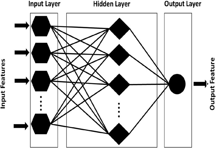
Figure 2. Illustration of the MLP algorithm.

Equation 9 represents the most commonly used activation function in MLPs: the sigmoid function.

${F\left(x\right)}_j=\frac{1}{1+e^{-S_j}}(9)$

Subsequently, the final output of the MLP is determined by applying Equation 10 to the computed outputs of each neuron in the hidden layer.

$y_j={F\left(x\right)}_j\left({\displaystyle \sum _{i=1}^n}{w}_{i,j}{I}_i+b_j\right)(10)$

It is evident from the equations that the weights and biases play an important role in shaping the characteristics of the MLP. Optimal values for the weights and biases need to be determined to achieve maximum performance in capturing the relationship between input and output variables.

2.3 Grey wolf optimization algorithm (GWO)

The grey wolf (GW), occupying the apex predator position in the food chain, demonstrates a strong propensity for group living. Each individual within the population assumes a specific role, contributing to establishing a strict social hierarchy, as illustrated in Figure 3.

Figure 3

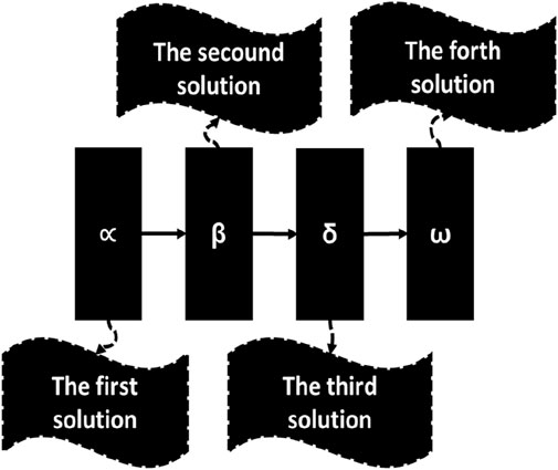
Figure 3. Illustration of the hierarchy of the GOW algorithm.

The first tier of this hierarchical structure comprises the highest-ranking leader of the grey wolves, referred to as ∝ (Tu et al., 2019). This ∝ individual holds the primary responsibility for making critical decisions about hunting strategies, habitat selection, and other relevant factors. Subsequently, the second tier consists of subordinate leaders within the grey wolf pack, β individuals (Xie et al., 2020). Their principal role involves managing the pack’s leadership, coordinating group activities, and fostering collaborations with other wolf packs (Prakash and Viswanathan, 2021; Wang et al., 2024). Within the third tier, we find the δ individuals, primarily tasked with monitoring the territorial boundaries, warning the wolf pack of potential dangers, and displaying care towards weaker or wounded members of the pack. Finally, the fourth tier encompasses the lowest-ranking individuals within the population, denoted as ω wolves. Despite their seemingly less prominent role, these omega wolves are indispensable in maintaining balance within the population’s internal relations. The leadership hierarchy of wolves plays a pivotal role in the hunting process. Initially, the grey wolves engage in search and tracking of prey. Subsequently, the alpha grey wolf leads the pack in encircling the prey from all directions. The alpha wolf then commands the beta and delta wolves to initiate the attack on the prey. If the prey manages to escape, the remaining wolves, situated at the rear, continue the pursuit and resume the attack (Cai et al., 2019; Shi et al., 2024). Ultimately, the grey wolves strive to capture their prey successfully.

The GWO simulates wolves’ leadership hierarchy and predatory behavior, harnessing their innate abilities such as searching, encircling, hunting, and other predation activities to optimize solutions. Assuming a population size of N wolves and a search area of d, the position of the ith wolf can be represented as Z_i = (Z_i1, Z_i2, Z_i3, … , Z_id). To mathematically model the social hierarchy of wolves, the fittest solution is designated as the ∝ wolf. In contrast, the second and third-best solutions are assigned as β and δ wolves, respectively. The remaining candidate solutions are considered as ω wolves. The prey’s position corresponds to the wolf’s location in the algorithm. The encircling behavior of grey wolves can be mathematically formulated as shown in Equations 11, 12.

$ϵ=\left|{2r}_i\times Z_P\left(t\right)-Z_c\left(t\right)\right|(11)$

$Z\left(t+1\right)=Z_P\left(t\right)-\left(2a{r}_2-2\left(1-\frac{1}{\partial \mathit{max}}\right)\right)\times F(12)$

In the given context, where t represents the current iteration, Z_p(t) signifies the position vector of the prey, and Z_P(t) denotes the position vector of a grey wolf.

When grey wolves successfully capture prey, the hunting process involves several steps. Firstly, the α wolf assumes the lead role, guiding the other wolves to encircle the prey. Subsequently, the α wolf coordinates the β and δ wolves to execute the capture of the prey. Given that the α, β, and δ wolves are in closest proximity to the prey, the location of the prey can be determined by their respective positions. The mathematical model representing this process is as Equations 13–19:

${ϵ}_{\alpha }=\left|{\left({2r}_i\right)}_1\times Z_{\alpha }\left(t\right)-Z_c\left(t\right)\right|(13)$

${ϵ}_{\beta }=\left|{\left({2r}_i\right)}_2\times Z_{\beta }\left(t\right)-Z_c\left(t\right)\right|(14)$

${ϵ}_{\delta }=\left|{\left({2r}_i\right)}_3\times Z_{\delta }\left(t\right)-Z_c\left(t\right)\right|(15)$

$Z_1=Z_{\alpha }\left(t\right)-\left(2a{r}_2-2\left(1-\frac{1}{\partial \mathit{max}}\right)\right)\times F_{\alpha }(16)$

$Z_2=Z_{\beta }\left(t\right)-\left(2a{r}_2-2\left(1-\frac{1}{\partial \mathit{max}}\right)\right)\times F_{\beta }(17)$

$Z_3=Z_{\delta }\left(t\right)-\left(2a{r}_2-2\left(1-\frac{1}{\partial \mathit{max}}\right)\right)\times F_{\delta }(18)$

$Z\left(t+1\right)=\frac{Z_1+Z_2+Z_3}{3}(19)$

The distance between the position vectors Z(t) and the α, β, and ω wolves is calculated using Equations 12–17. Subsequently, the calculation of the movement of the wolves towards the prey is determined by Equation 19.

2.4 Grasshopper optimization algorithm (GOA)

Grasshoppers belong to the insect species and are recognized as pests due to the damage they inflict on crops (Amaireh et al., 2022). Despite their seemingly solitary nature, grasshoppers are one of the largest animal groups on Earth and can threaten farmers. One remarkable aspect of their behavior is their social tendencies, which manifest during both their early stages of development and adulthood (Shukla, 2021). Millions of grasshopper larvae exhibit synchronized movement, resembling rolling behavior, as they voraciously consume plants along their path. Grasshoppers exhibit slow movements and short strides as their distinguishing features.

In contrast, mature grasshopper communities exhibit short and sudden movements. A prominent characteristic of their social behavior is the search for food resources. Inspired by the natural behavior of grasshoppers, the GOA logically divides the search process into two phases: exploration and exploitation (Sui et al., 2020).

During the exploration phase, search agents are encouraged to make abrupt movements, while in the exploitation phase, they tend to focus on local movements. The mathematical model simulating grasshopper social behavior is described by the following Equation 20:

$Z_i=M_i+N_i+O_i(20)$

where Z_i is the location of the grasshopper, M_i represents the influence of wind, N_i denotes social interaction, and O_i corresponds to the gravitational effect on the grasshopper (r1, r2, and r3 are between 0–1). To introduce randomness, the equation is modified as Equation 21:

$Z_i=r_1{\displaystyle \sum _{j=1}^n}s\left(\left|Z_j-Z_i\right|\times \frac{Z_j-Z_i}{\left|Z_j-Z_i\right|}\right)-r_{2}g\widehat{e_g}-r_{3}g\widehat{e_w}(21)$

The symbol g represents the gravitational constant, while the symbol êg represents a unit vector that indicates the direction towards the center of the Earth. The you represent a constant displacement, and êw represents a unit vector perpendicular to the wind’s direction.

2.5 LSSVM-GOA/GWA algorithm

The flowchart diagrams displayed in Figure 4 provide a comprehensive visual representation of the sequential steps inherent in the LSSVM-GOA/GWO models. These models rely on the precise manipulation of control parameters within the LSSVM RBF kernel function, as they are paramount in achieving optimal prediction performance for LSSVM SMW. Determining these important control parameters is accomplished by leveraging the capabilities of either a GOA or GWO optimizer. The specific control parameters that the GOA or GWO algorithms have determined to be the best for use in the LSSVM model are listed in Table 2, along with the associated RBF control parameters.

Figure 4

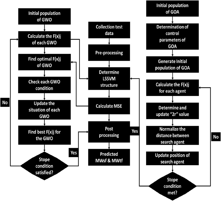
Figure 4. Flowchart diagram of LSSVM-GOA/GWO models for predicting MWsf and MWtf to determine SMW.

Table 2

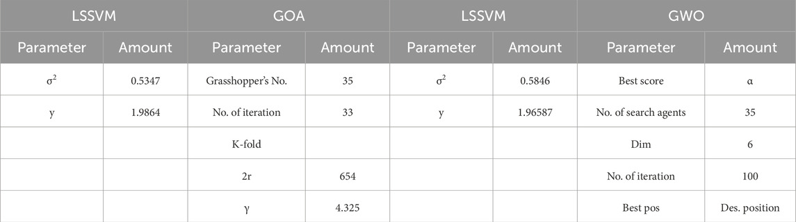
Table 2. Determination control parameters for combining the LSSVM with GOA and GWO models.

2.6 MLP-GOA/GWA algorithm

Figure 5 presents meticulously crafted flowchart diagrams, providing a comprehensive visual representation of the step-by-step processes intrinsic to the MLP-GOA/GWO models. These models rely extensively on the precise manipulation of control parameters within the MLP function, as they hold utmost significance in achieving the highest level of prediction performance for MLP SMW. These important control parameters are determined by harnessing the advanced capabilities of either a GOA or GWO optimizer. To further enhance the implementation of the MLP algorithm, Table 3 outlines and enumerates the specific control parameters identified as optimal by the GOA or GWO algorithms in the MLP algorithm.

Figure 5

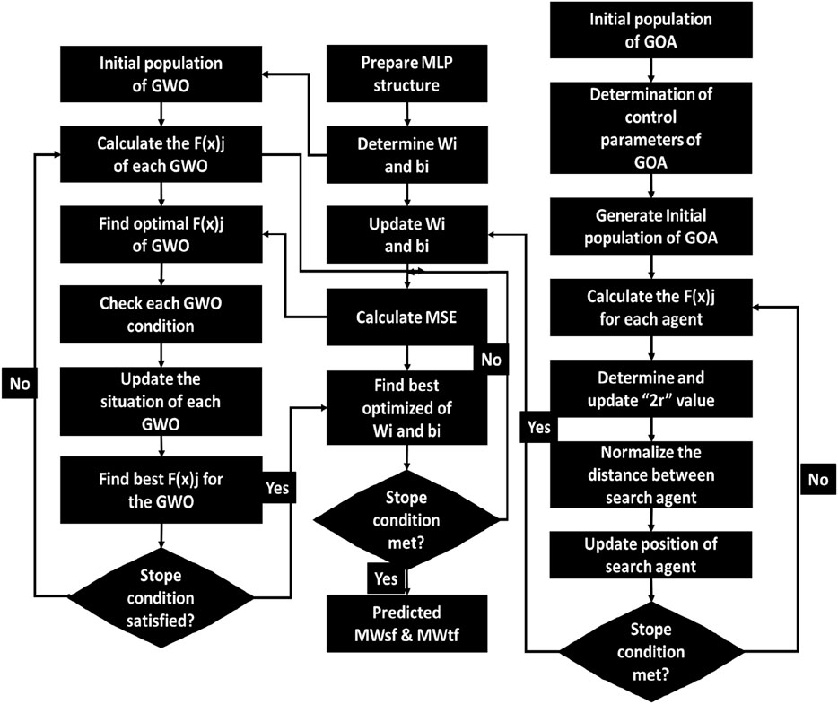
Figure 5. Flowchart diagram of MLP-GOA/GWO models for predicting MWsf and MWtf to determine SMW.

Table 3

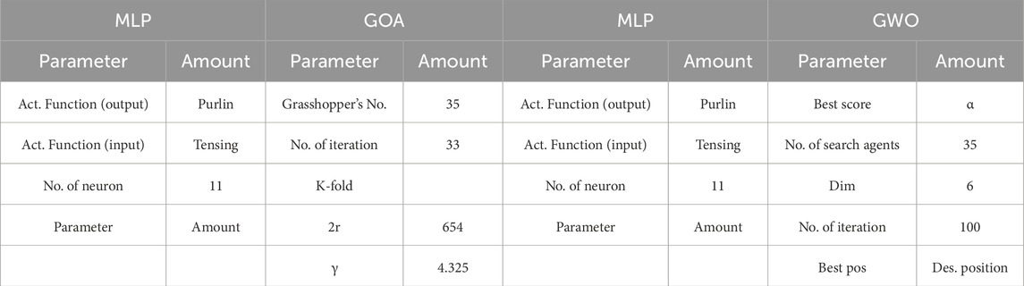
Table 3. Determination of control parameters for combining the MLP with GOA and GWO models.

While the control parameters (e.g., σ², γ, iteration counts, population sizes) listed in Tables 2 and 3 were optimized using GWO/GOA, their sensitivity was evaluated through iterative tuning. For instance, varying σ² in the LSSVM kernel by ±20% resulted in RMSE fluctuations of <5%, indicating robustness to minor deviations. Similarly, increasing the number of grasshoppers or wolves beyond 35 marginally improved accuracy (<1% R² gain) at the cost of computational efficiency. The selected parameters represent a balance between performance and practicality. Future work could explore dynamic parameter adaptation for further optimization.

2.7 K-fold cross-validation (KFCV)

The KFCV is a widely utilized technique in the field of machine learning, particularly for numerical datasets. It is an effective method for evaluating and fine-tuning models (Cheng et al., 2022; Pannakkong et al., 2022). This technique involves dividing the dataset into K subsets, or folds, enabling the iterative training and evaluation of the model on different subsets. By assessing the model’s performance across multiple validation sets, KFCV provides a robust measure of its effectiveness and generalizability. It aids in optimizing hyperparameters, reducing the risk of overfitting, and gaining valuable insights into the model’s behavior (Ziggah et al., 2019). Moreover, this technique maximizes data utilization and effectively addresses performance variability, making it an indispensable tool for assessing and comparing model performance on numerical datasets. The flowchart representation of the k-fold validation process is visually depicted in Figure 6.

Figure 6

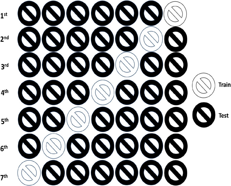
Figure 6. K-fold diagram for prediction of MWsf and MWtf to determine SMW.

A stratified 10-fold cross-validation was employed to ensure balanced representation of data subsets. The dataset was partitioned into 10 folds, with 9 folds used for training and one for validation iteratively. Stratification preserved the distribution of MWsf and MWtf targets across folds, avoiding skewed evaluations. Model performance metrics were averaged across all folds to assess generalizability. This approach minimizes overfitting by validating the model on distinct subsets, ensuring robustness against data variability. Figure 6 illustrates the KFCV workflow, emphasizing the iterative cycle of training, validation, and aggregation. Each fold’s validation results contribute to a consolidated performance metric, aligning with best practices for model evaluation in geochemical drilling applications.

3 Data gathering for model construction

In order to forecast the commonly used geochemical drilling parameter SMW utilizing the combined methods LSSVM-GWO, MLP-GWO, LSSVM-GOA, and MLP-GOA data sets linked to three wells V1, V2, and V3 in one of the oil fields in the Middle East have been employed. Due to the V1 well’s size and distribution, hybrid artificial intelligence models have been created using this well’s data. The information about well V1 contains 901 data with a 0.2 m interval; the information about well V2 contains 983 data with a 0.2 m interval; and the information about well V3 contains 936 data with a 0.2 m interval. 70% of the data from wells V1 and V2 were randomly chosen to be the train data set, 15% the test data set, and the remaining 15% the validation data to develop these models.

Table 4 reports the information and purity related to the data values used in this article, which include LSSVM-GWO, MLP-GWO, LSSVM-GOA, and MLP-GOA. Certain data variables hold immense significance when forecasting and determining the properties of SMW. These data variables include drilling time (t), caliper (cP), weight on bit (WOB), flow rate (Q), retort solid (RS), fan 600/fan 300 (F600/F300), gel10min/gel10s (G10min/G10s), pump discharge pressure (Pw), and rotations per minute (RPM).

Table 4

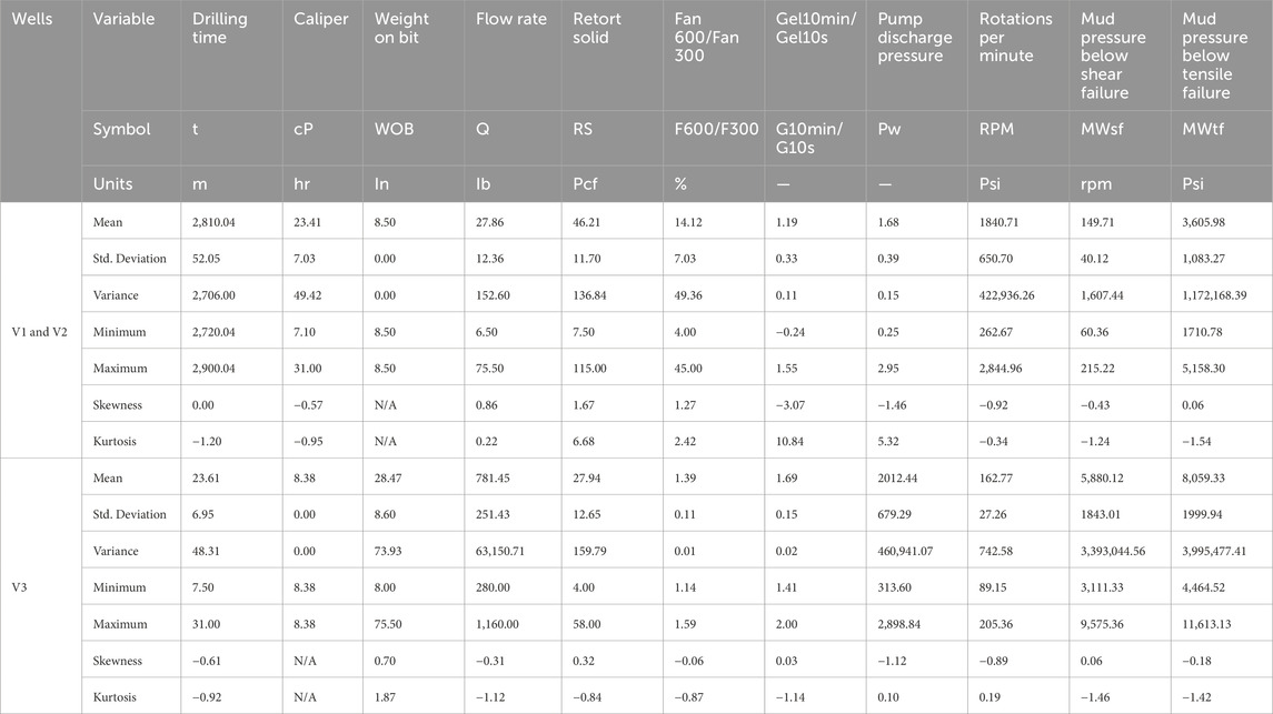
Table 4. Well-statistical reports on data were used to build four HMLs (LSSVM-GWO, MLP-GWO, LSSVM-GOA, and MLP-GOA) to predict MWsf and MWtf to determine SMW.

In addition to the data above, two specific border mud pressures below shear failure (MWsf) and mud pressure below tensile failure (MWtf) are also important in determining SMW properties. These two parameters indicate the maximum pressure the drilling mud can withstand before breaking down, which is essential in determining the characteristics and behavior of SMW during drilling operations. Therefore, selecting and analyzing these data variables are critical in predicting and determining the properties of SMW.

4 Discussion of results and comparison methods

This article uses LSSVM-GWO, MLP-GWO, LSSVM-GOA, and MLP-GOA methods to forecast the SMW. To assess and compare the performance of these artificial intelligence methods, we utilize a benchmark equation and statistical techniques, presented as Equations 22–24. Detailed reports regarding training, testing, and validation data outcomes are provided in Tables 5, 6. Based on these tables, the outcomes of the subsets associated with training, testing, and validation have been bifurcated into MWsf and MWtf divisions. One of the key rationales for incorporating the upper and lower limits of mud pressure as two parameters in this study stems from the fact that the SMW value resides between these two thresholds of mud pressure. Consequently, this article employs artificial intelligence techniques to leverage both significant parameters effectively.

$\text{RMSE}=\sqrt{\frac{1}{\mathrm{n}}{\displaystyle \sum _{\mathrm{i}=1}^{\mathrm{n}}}{\left({{\text{SMW}}_{\mathrm{M}.}}_{\mathrm{i}}-{{\text{SMW}}_{\mathrm{P}.}}_{\mathrm{i}}\right)}^2}(22)$

$\text{NRMSE}=\frac{\sqrt{\frac{1}{\mathrm{n}}{\displaystyle {\sum }_{\mathrm{i}=1}^{\mathrm{n}}}{\left({{\text{SMW}}_{\mathrm{M}.}}_{\mathrm{i}}-{{\text{SMW}}_{\mathrm{P}.}}_{\mathrm{i}}\right)}^2}}{{{\text{SMW}}_{\mathrm{M}.}}_{\mathit{max}}-{{\text{SMW}}_{\mathrm{M}.}}_{\mathit{min}}}(23)$

${\mathrm{R}}^2=1-\frac{{\displaystyle {\sum }_{\mathrm{i}=1}^{\mathrm{N}}}{\left({{\text{SMW}}_{\mathrm{M}.}}_{\mathrm{i}}-{{\text{SMW}}_{\mathrm{P}.}}_{\mathrm{i}}\right)}^2}{{\displaystyle {\sum }_{\mathrm{i}=1}^{\mathrm{N}}}{\left({{\text{SMW}}_{\mathrm{P}.}}_{\mathrm{i}}-\frac{{\sum }_{\mathrm{I}=1}^{\mathrm{n}}{{\text{SMW}}_{\mathrm{M}.}}_{\mathrm{i}}}{\mathrm{n}}\right)}^2}(24)$

Table 5

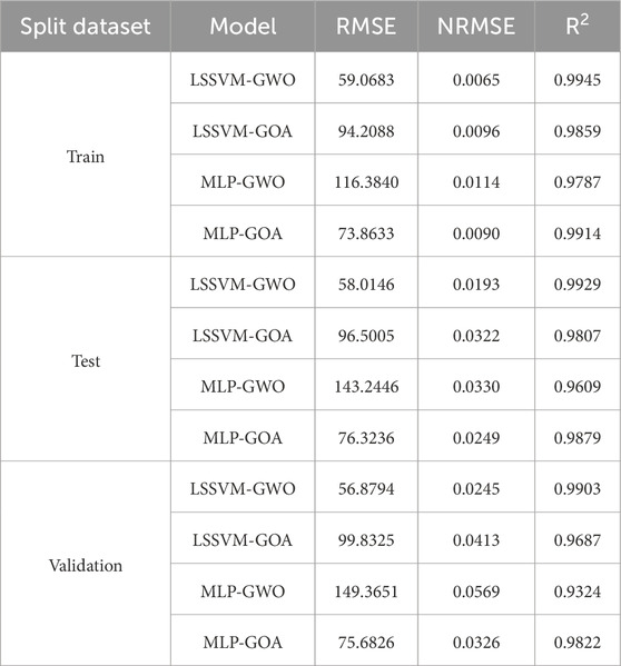
Table 5. Determination of statical parameters based on testing, training, and validation results based on V1 and V2 well data sets for prediction of MWsf by four HML.

Table 6

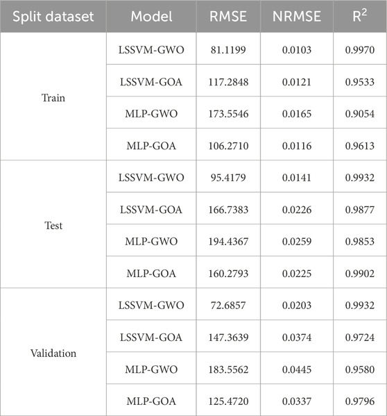
Table 6. Determination of statical parameters based on testing, training, and validation results based on V1 and V2 well data sets for prediction of MWtf by four HML.

The outcomes of the training, test, and validation datasets for predicting MWtf and MWsf using four hybrid machine learning models (LSSVM-GWO, MLP-GWO, LSSVM-GOA, and MLP-GOA) are provided in Tables 5, 6. The two most relevant parameters, R2 and RMSE, are employed to establish a suitable criterion for comparing these methods. R² and RMSE are influential and significant metrics for evaluating and contrasting the models. Analyzing the findings in Table 5 reveals that the LSSVM-GWO model exhibits superior accuracy in predicting MWsf compared to the LSSVM-GOA, MLP-GWO, and MLP-GOA models. The LSSVM-GWO algorithm yields the following results: RMSE = 59.0683 and R² = 0.9945 for the training set, RMSE = 58.0146 and R² = 0.9929 for the test set, and RMSE = 56.8794 and R² = 0.9903 for the validation set. Furthermore, Table 6 also illustrates that the LSSVM-GWO model demonstrates higher accuracy in predicting MWtf than the LSSVM-GOA, MLP-GWO, and MLP-GOA models. The results indicate that for the training set, the LSSVM-GWO algorithm achieves RMSE = 81.1199 and R² = 0.9970, while for the test set, it attains RMSE = 95.4179 and R² = 0.9929. Lastly, for the validation set, the LSSVM-GWO algorithm yields RMSE = 72.6857 and R² = 0.9932.

One of the important aspects of evaluating mathematical forecasting methods lies in using statistical metrics, such as R², to assess their performance. Figure 7 provides insights into the graphical analysis conducted for predicting MWsf using the test dataset. Through an examination of the R² value and the proximity of the predicted points to the trendline in the cross-plot of measured and predicted values, it becomes apparent that the LSSVM-GWO algorithm exhibits superior accuracy compared to the MLP-GWO, LSSVM-GOA, and MLP-GOA algorithms. Similarly, Figure 8 offers a glimpse into the analysis for predicting MWtf using the test dataset. By evaluating the R2 value and the proximity of the predicted points to the trendline in the cross-plot, it is evident that the LSSVM-GWO algorithm outperforms the MLP-GWO, LSSVM-GOA, and MLP-GOA algorithms in terms of accuracy.

Figure 7

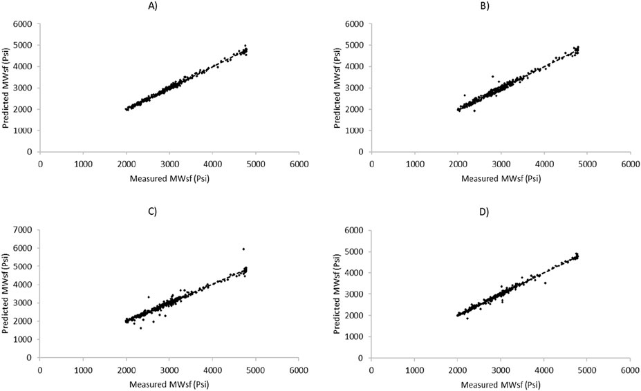
Figure 7. Cross-plot diagram for prediction of MWsf based on test dataset by four HML models: (A) LSSVM-GWO, (B) LSSVM-GOA, (C) MLP-GWO, (D) MLP-GOA.

Figure 8

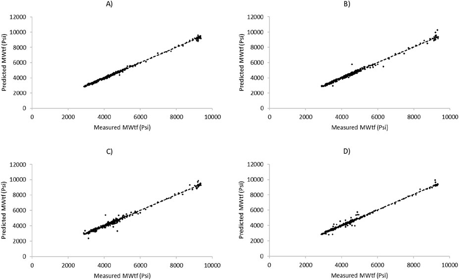
Figure 8. Cross-plot diagram for prediction of MWtf based on test dataset by four HML models: (A) LSSVM-GWO, (B) LSSVM-GOA, (C) MLP-GWO, (D) MLP-GOA.

Figures 9, 10 present the relative error diagrams for predicting MWsf and MWtf using the test dataset and four HML models, namely LSSVM-GWO, MLP-GWO, LSSVM-GOA, and MLP-GOA. These figures illustrate the error ranges associated with each algorithm, allowing for a comprehensive comparison. In Figure 9, the error ranges for the LSSVM-GWO, MLP-GWO, LSSVM-GOA, and MLP-GOA algorithms are [−4.643–5.006], [−19.017–25.878], [−31.441–30.964], and [−17.015–10.821], respectively. Similarly, Figure 10 displays the error ranges for the LSSVM-GWO, MLP-GWO, LSSVM-GOA, and MLP-GOA algorithms as [−4.927–9.149], [−26.817–15.624], [−32.664–30.451], and [−18.124–19.033], respectively. The LSSVM-GWO model achieves R² > 0.99 for both MWsf and MWtf, surpassing standalone ML methods like SVM-RBF (R² = 0.9329; Zahiri et al., 2019) and ANN (R² = 0.998; Phan et al., 2020). This improvement stems from GWO’s ability to optimize LSSVM parameters (e.g., kernel width, regularization), enabling robust handling of noise and nonlinearity in drilling data. Additionally, unlike conventional geomechanical models (e.g., Mogi-Coulomb), which require explicit stress-strain relationships, our data-driven approach adapts to heterogeneous formations without prior assumptions. These figures demonstrate that LSSVM-GWO algorithm exhibits a higher level of performance accuracy with a lower error area compared to others. However, further improvements might be achievable through advanced hyperparameter tuning techniques like Bayesian Optimization, which systematically balances exploration and exploitation while avoiding local optima.

Figure 9

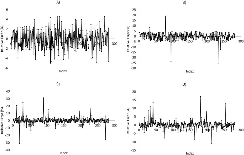
Figure 9. Relative error diagram versus data number for prediction of MWsf based on test dataset by four HML models: (A) LSSVM-GWO, (B) LSSVM-GOA, (C) MLP-GWO, (D) MLP-GOA.

Figure 10

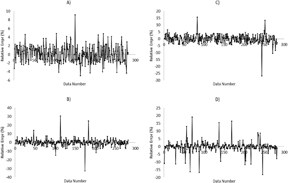
Figure 10. Relative error diagram versus data number for prediction of MWtf based on test dataset by four HML models: (A) LSSVM-GWO, (B) LSSVM-GOA, (C) MLP-GWO, (D) MLP-GOA.

Figures 11, 12 illustrate the histograms of MWsf and MWtf prediction errors obtained from four robust HML models: LSSVM-GWO, MLP-GWO, LSSVM-GOA, and MLP-GOA. The histogram shows that the MWsf prediction errors exhibit a symmetric distribution centered around zero. Notably, for the LSSVM-GWO algorithm, the error distribution appears to follow a normal distribution. However, the statistical error distributions of the other algorithms, MLP-GWO, LSSVM-GOA, and MLP-GOA, display non-normal patterns when observed through a scan view.

Figure 11

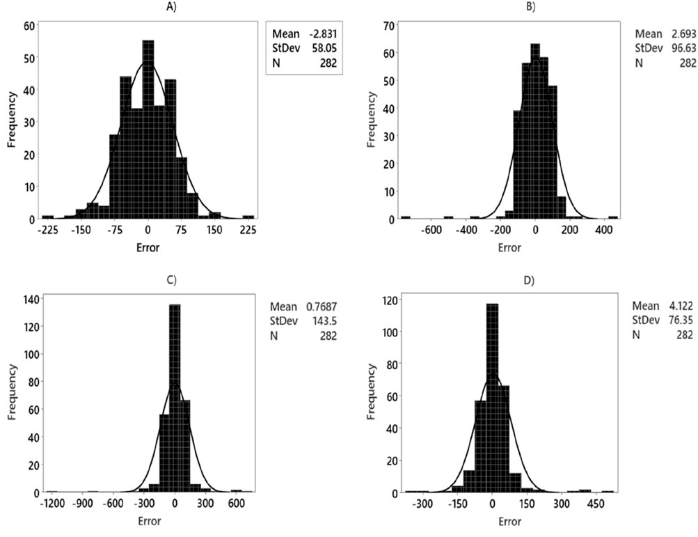
Figure 11. Histogram diagram versus for prediction of MWsf based on test dataset by four HML models: (A) LSSVM-GWO, (B) LSSVM-GOA, (C) MLP-GWO, (D) MLP-GOA.

Figure 12

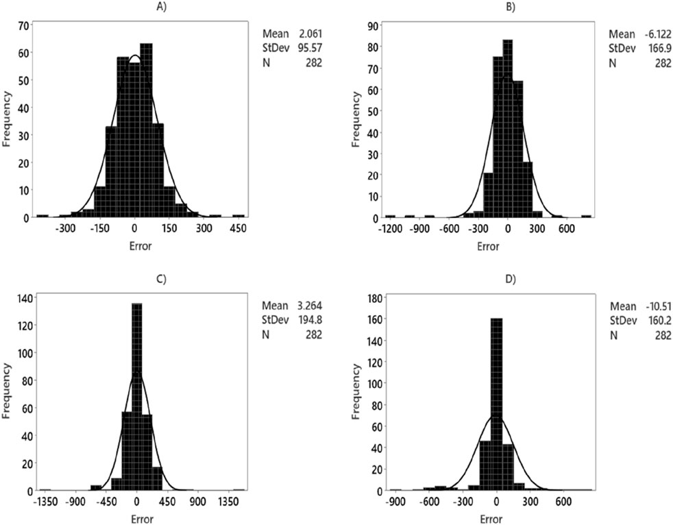
Figure 12. Histogram diagram versus for prediction of MWtf based on test dataset by four HML models: (A) LSSVM-GWO, (B) LSSVM-GOA, (C) MLP-GWO, (D) MLP-GOA.

Based on the graphical information presented in Figures 13, 14, as well as the data provided in Tables 5, 6, the evaluation of MWsf and MWtf prediction using four HML algorithms (LSSVM-GWO, MLP-GWO, LSSVM-GOA, and MLP-GOA) reveals contrasting outcomes for the performance metrics of RMSE and R². These figures demonstrate that an increase in R² corresponds to a decrease in RMSE, indicating a stronger correlation between the predicted and actual values of MWsf and MWtf. Consequently, a lower RMSE signifies a smaller average error in the predictions. The findings support the conclusion that the LSSVM-GWO algorithm outperforms the MLP-GWO, LSSVM-GOA, and MLP-GOA algorithms regarding MWsf and MWtf prediction accuracy. The higher R² values and lower RMSE values associated with the LSSVM-GWO algorithm validate its superior performance compared to the other algorithms. Therefore, the comparative analysis establishes the following accuracy ranking: LSSVM-GWO > MLP-GOA > LSSVM-GOA > MLP-GWO.

Figure 13

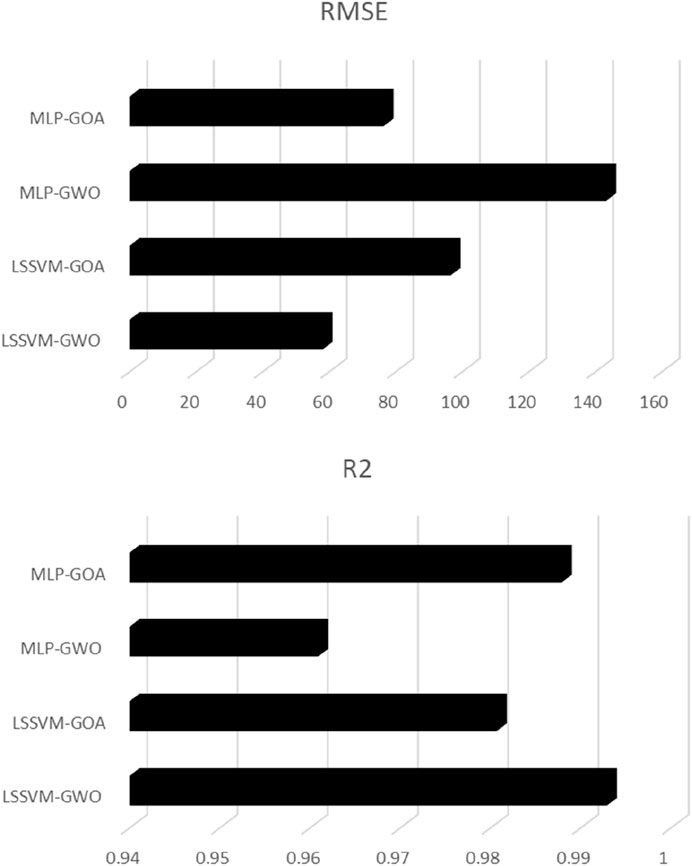
Figure 13. Error diagram for prediction of MWsf based on test dataset by four HML models.

Figure 14

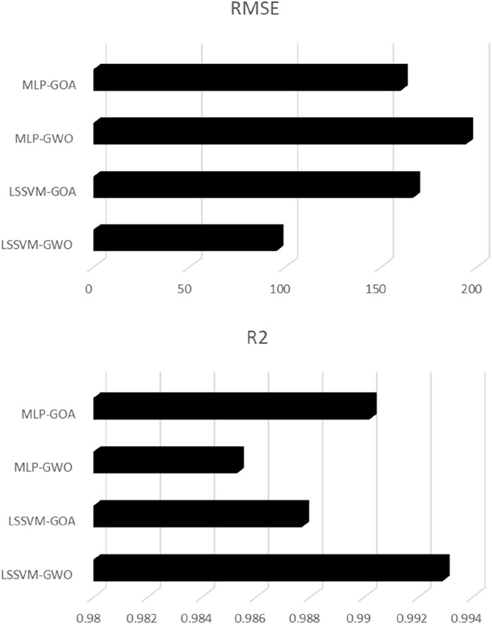
Figure 14. Error diagram for versus for prediction of MWtf based on test dataset by four HML models.

5 Evaluation, generalization, and development algorithm

Pearson’s correlation coefficient (R) is a widely used statistical measure for assessing the relationship between input-independent and output-dependent variables, such as MWsf and MWtf. This R, which ranges from −1 to +1, provides insights into the strength and direction of the correlation between the variables. A value of +1 indicates a strong positive correlation, −1 indicates a strong negative correlation, and a value close to 0 suggests a weak or no significant correlation. Equation 25 outlines the calculation of R, enabling researchers to evaluate the linear association between two variables quantitatively. By utilizing R, researchers can determine the extent to which changes in one variable are linked to changes in another variable, thereby assessing the impact of input-independent variables on the output-dependent variables, MWsf and MWtf.

$R=\frac{{\displaystyle {\sum }_{i=1}^n}\left({\theta }_i-\overline{\theta }\right)\left({\partial }_i-\overline{\partial }\right)}{\sqrt{{\sum }_{i=1}^n{\left({\theta }_i-\overline{\theta }\right)}^2}\sqrt{{\sum }_{i=1}^n{\left({\partial }_i-\overline{\partial }\right)}^2}}(25)$

The heat map in Figure 15 provides a valuable tool for comparing the R and gaining insights into the relationships between the input variables and MWsf and MWtf.

Figure 15

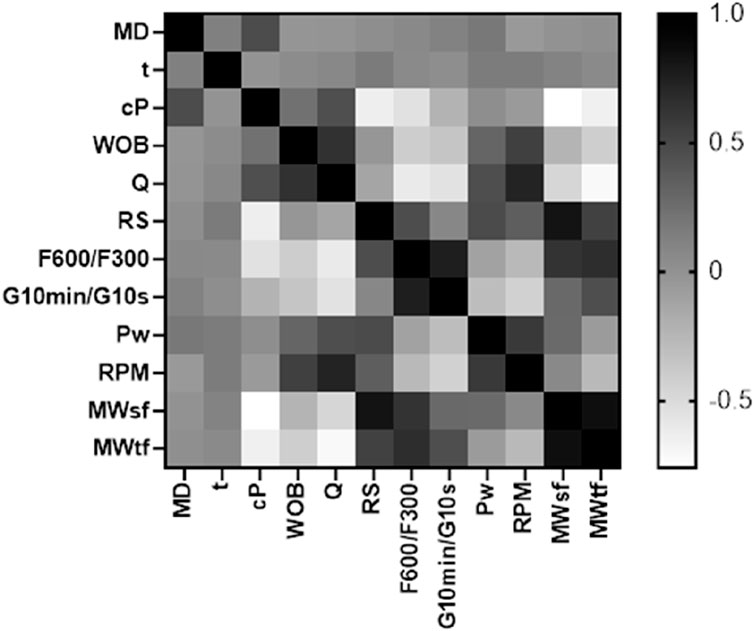
Figure 15. Heat diagram for determination of the effect of each variable for prediction MWtf and MWtf to determine SMW based on four HML models.

The analysis of MWsf reveals several significant correlations with the input variables. There are negative correlations with MD, cP, WOB, and Q, indicating an inverse relationship with MWsf. Conversely, positive correlations are observed with t, Rs, F600/F300, G10min/G10s, Pw, and RPM (see Equation 26). Based on R, the variables Q, RS, and F600/F300 have a higher impact on MWsf.

$MWsf\propto \frac{t,Rs,F600/F300,G10\mathit{min}/G10s,Pw,RPM}{MD,cP,WOB,Q}(26)$

Significant correlations regarding MWtf are observed with the input variables. Negative correlations with cP, WOB, Q, Pw, and RPM indicate an inverse relationship with MWtf. Conversely, positive correlations are observed with MD, t, Rs, F600/F300, G10min/G10s, Pw, and RPM (see Equation 27). Based on R, the variables WOB, Q, Rs, F600/F300, and G10min/G10s have a higher impact on MWtf.

$MWtf\propto \frac{MD,t,Rs,F600/F300,G10\mathit{min}/G10s}{cP,WOB,Q,Pw,RPM}(27)$

When analyzing the hybrid artificial intelligence algorithms LSSVM-GWO, MLP-GWO, LSSVM-GOA, and MLP-GOA for predicting the two key parameters MWtf and MWtf and obtaining the prediction of SMW, it was found that the LSSVM-GWO algorithm outperforms the others in terms of accuracy. Initially, these algorithms were developed using data from two wells, V1 and V2. However, to generalize and improve the LSSVM-GWO algorithm and evaluate its accuracy for another well, namely V3, data from well V3 were utilized. The results obtained for this algorithm are displayed in Figure 16 and Table 7. These findings demonstrate that the algorithm effectively predicts the important parameters MWtf and MWtf, ultimately providing an accurate estimation of SMW (RMSE_MWsf = 50.2601 and RMSE_MWtf = 70.8868). This is particularly significant in the drilling industry as it helps mitigate costs arising from losses or casing collapses due to incorrect or delayed identification of SMW. To further validate the LSSVM-GWO model’s reliability, well V3 data (n = 936) were used to test generalization. Figure 16 shows minimal deviation (RMSE <70 Psi), confirming the model’s robustness even for wells not included in training. Outliers in V3 (e.g., MWsf > 9,000 Psi) were linked to rare geological conditions (e.g., abrupt caliper changes), which future work could address by incorporating real-time lithology data.

Figure 16

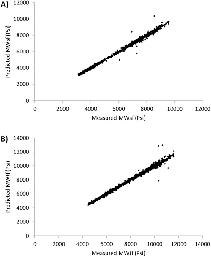
Figure 16. Cross plot diagram for prediction of (A) MWsf and (B) MWtf to generalize and develop LSSVM-GWO based on V3 well’s dataset.

Table 7

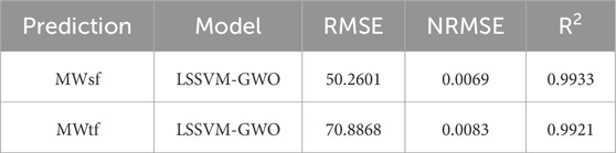
Table 7. Determination of statical parameters for prediction of MWsf and MWtf to generalize and develop LSSVM-GWO based on V3 well’s dataset.

6 Future work

In this article, the best algorithm for predicting a safe mud window is LSSVM-GWO. We suggest that this algorithm can be used for important studies, such as thermodynamic constitutive modeling (Bai et al., 2025a; Bai et al., 2025b), graph neural networks and collaborative filtering (Shi et al., 2025a), and visual question answering (Han et al., 2025). Additionally, it shows potential for enhancing vehicle dynamics and control systems (Cao et al., 2024; Li et al., 2020a; Li et al., 2021a; Li et al., 2020b; Li et al., 2021b; Li et al., 2020c; Li et al., 2020d; Ma et al., 2022; Xie et al., 2023; Xie et al., 2024), as well as environmental modeling and optimization (Yang et al., 2011; Zhao et al., 2012; Zhiquan et al., 2015). Furthermore, the algorithm can be applied to combustion control and optimization (Gao et al., 2017) and biomedical research (Yuan et al., 2009).

7 Limitation

While the LSSVM-GWO algorithm demonstrated superior performance, this study has several limitations. First, the model’s generalizability relies heavily on the quality and representativeness of the geochemical drilling log data from Middle Eastern carbonate reservoirs, which may not fully capture geological variability in other regions. Second, the computational complexity of hybridizing LSSVM with optimization algorithms like GWO/GOA could pose challenges for real-time applications in large-scale drilling operations. Third, the study assumes consistent availability of all input parameters (e.g., retort solids, fan readings) during drilling, which may not always be feasible in field conditions. Additionally, the model’s performance is contingent on the hyperparameters selected for optimization (e.g., kernel functions, population size), requiring careful tuning that may demand domain expertise. Finally, the lack of explicit integration with physics-based geomechanical models limits interpretability of the machine learning outputs for operational decision-making. Future work should address these limitations by testing the algorithm on diverse geological formations, optimizing computational efficiency, and hybridizing data-driven approaches with mechanistic models to enhance robustness and transparency.

8 Conclusion and recommendation

In order to determine the value of the safe mud window (SMW), a comprehensive analysis was conducted using data from three wells (V1, V2, and V3) located in an oil field in the Middle East. The primary objective of this analysis was to predict the parameters MWsf and MWtf by considering various variables, including drilling time (t), caliper (cP), weight on bit (WOB), flow rate (Q), retort solids (RS), fan 600/fan 300 (F600/F300), gel10min/gel10s (G10min/G10s), pump discharge pressure (Pw), and rotations per minute (RPM). To achieve this, a combination of machine learning algorithms, namely Least Squares Support Vector Machine (LSSVM) and Multilayer Perceptron (MLP) networks, along with optimization techniques such as Gray Wolf Optimization (GWO) and Grasshopper Optimization Algorithm (GOA), were employed. The performance of four algorithms, LSSVM-GWO, MLP-GWO, LSSVM-GOA, and MLP-GOA, was thoroughly analyzed, revealing that the LSSVM-GWO algorithm exhibited superior accuracy compared to the others. The calculated error values for the test data in the LSSVM-GWO algorithm were RMSE (MWsf) = 58.0146 with an R² value of 0.9929 and RMSE (MWtf) = 95.4179 with an R² value of 0.9932. Furthermore, the accuracy of the LSSVM-GWO algorithm was maintained when data from an additional well (V3) was used to develop and generalize the algorithm. The LSSVM-GWO hybrid algorithm offers several advantages: enhanced accuracy, parameter-free optimization, faster convergence, and versatility. Pearson correlation analysis revealed significant associations between MWsf and the input variables. The analysis demonstrated several noteworthy correlations with the input variables for MWsf. Negative correlations were observed with MD, cP, WOB, and Q, indicating an inverse relationship with MWsf. Conversely, positive correlations were observed with t, Rs, F600/F300, G10min/G10s, Pw, and RPM. Based on the correlation coefficients, the variables Q, RS, and F600/F300 have a higher impact on MWsf. Regarding MWtf, significant correlations with the input variables were observed. Negative correlations were found with cP, WOB, Q, Pw, and RPM, indicating an inverse relationship with MWtf. Conversely, positive correlations were observed with MD, t, Rs, F600/F300, G10min/G10s, Pw, and RPM. Based on the correlation coefficients, the variables WOB, Q, Rs, F600/F300, and G10min/G10s have a higher impact on MWtf. Future research should focus on expanding the applicability of the LSSVM-GWO algorithm to diverse reservoir types (e.g., shale, sandstone) to validate its robustness across varying geological conditions. Integrating real-time drilling data streams, such as downhole sensor measurements or seismic attributes, could further refine predictions. Enhancing computational efficiency through lightweight model architectures or parallel processing frameworks would enable real-time SMW estimation during drilling operations. Additionally, exploring hybrid models that combine LSSVM-GWO with deep learning techniques (e.g., convolutional neural networks) or physics-informed constraints could improve interpretability and generalization. Investigating the impact of environmental factors, such as temperature gradients or formation heterogeneity, on SMW prediction accuracy also merits attention. Finally, deploying the algorithm in cloud-based platforms for collaborative, multi-well analysis could optimize reservoir management strategies at scale.

Data availability statement

The data analyzed in this study is subject to the following licenses/restrictions: The corresponding author are willing to provide access to the data upon reasonable requests for academic purposes. Requests to access these datasets should be directed to Yunliang Yu; eXV5dW5saWFuZ0BqbHUuZWR1LmNu.

Author contributions

HC: Conceptualization, Formal Analysis, Funding acquisition, Investigation, Methodology, Project administration, Resources, Software, Validation, Writing–original draft, Writing–review and editing. YY: Conceptualization, Data curation, Funding acquisition, Investigation, Resources, Software, Supervision, Validation, Visualization, Writing–original draft, Writing–review and editing. YL: Formal Analysis, Funding acquisition, Investigation, Methodology, Project administration, Resources, Supervision, Visualization, Writing–original draft, Writing–review and editing. XG: Data curation, Formal Analysis, Methodology, Project administration, Resources, Software, Validation, Visualization, Writing–original draft, Writing–review and editing.

Funding

The author(s) declare financial support was received for the research, authorship, and/or publication of this article. The work was supported by the State Scholarship Fund sponsored by the China Scholarship Council (No.201506175098).

Conflict of interest

The authors declare that the research was conducted in the absence of any commercial or financial relationships that could be construed as a potential conflict of interest.

Generative AI statement

The author(s) declare that no Generative AI was used in the creation of this manuscript.

Publisher’s note

All claims expressed in this article are solely those of the authors and do not necessarily represent those of their affiliated organizations, or those of the publisher, the editors and the reviewers. Any product that may be evaluated in this article, or claim that may be made by its manufacturer, is not guaranteed or endorsed by the publisher.

References

Abdelghany, W. K., Radwan, A. E., Elkhawaga, M. A., Wood, D. A., Sen, S., and Kassem, A. A. (2021). Geomechanical modeling using the depth-of-damage approach to achieve successful underbalanced drilling in the Gulf of Suez Rift Basin. J. Petroleum Sci. Eng. 202, 108311. doi:10.1016/j.petrol.2020.108311

CrossRef Full Text | Google Scholar

Al-Nutaifi, A. M. (2019). “Wellbore instability analysis in a highly fractured carbonate gas reservoirs,” in International Petroleum Technology Conference, Kuala Lumpur, Malaysia, December 2014.

Google Scholar

Amaireh, A. A., Al-Zoubi, A. S., and Dib, N. I. (2022). A new hybrid optimization technique based on antlion and grasshopper optimization algorithms. Evol. Intell. 16, 1383–1422. doi:10.1007/s12065-022-00749-4

CrossRef Full Text | Google Scholar

Aslannezhad, M., Khaksar manshad, A., and Jalalifar, H. (2016). Determination of a safe mud window and analysis of wellbore stability to minimize drilling challenges and non-productive time. J. Petroleum Explor. Prod. Technol. 6, 493–503. doi:10.1007/s13202-015-0198-2

CrossRef Full Text | Google Scholar

Bai, B., Wu, H., Nie, Q., Liu, J., and Jia, X. (2025a). Granular thermodynamic migration model suitable for high-alkalinity red mud filtrates and test verification. Int. J. Numer. Anal. Methods Geomechanics. doi:10.1002/nag.3946

CrossRef Full Text | Google Scholar

Bai, B., Zhang, B., Chen, H., and Chen, P. (2025b). A novel thermodynamic constitutive model of coarse-grained soils considering the particle breakage. Transp. Geotech. 50, 101462. doi:10.1016/j.trgeo.2024.101462

CrossRef Full Text | Google Scholar

Cai, Z., Gu, J., Luo, J., Zhang, Q., Chen, H., Pan, Z., et al. (2019). Evolving an optimal kernel extreme learning machine by using an enhanced grey wolf optimization strategy. Expert Syst. Appl. 138, 112814. doi:10.1016/j.eswa.2019.07.031

CrossRef Full Text | Google Scholar

Cao, Y., Xie, Z., Li, W., Wang, X., Wong, P. K., and Zhao, J. (2024). Combined path following and direct yaw-moment control for unmanned electric vehicles based on event-triggered T–S fuzzy method. Int. J. Fuzzy Syst. 26, 2433–2448. doi:10.1007/s40815-024-01717-z

CrossRef Full Text | Google Scholar

Cheng, J., Kuang, H., Zhao, Q., Wang, Y., Xu, L., Liu, J., et al. (2022). DWT-CV: dense weight transfer-based cross validation strategy for model selection in biomedical data analysis. Future Gener. Comput. Syst. 135, 20–29. doi:10.1016/j.future.2022.04.025

CrossRef Full Text | Google Scholar

Fu, S., Hou, B., Xia, Y., Chen, M., Wang, S., and Tan, P. (2022). The study of hydraulic fracture height growth in coal measure shale strata with complex geologic characteristics. J. Petroleum Sci. Eng. 211, 110164. doi:10.1016/j.petrol.2022.110164

CrossRef Full Text | Google Scholar

Gao, J., Wu, Y., and Shen, T. (2017). On-line statistical combustion phase optimization and control of SI gasoline engines. Appl. Therm. Eng. 112, 1396–1407. doi:10.1016/j.applthermaleng.2016.10.183

CrossRef Full Text | Google Scholar

Ghorbani, H., Ghorbani, P., Ghorbani, S., Khlghatyan, N., Babayan, B. G., and Koczy, A. V. (2022). A robust approach for estimation of the bone age. IEEE, 000385–000390. doi:10.1109/sisy56759.2022.10036283

CrossRef Full Text | Google Scholar

Ghorbani, H., Krasnikova, A., Ghorbani, P., Ghorbani, S., Hovhannisyan, H. S., Minasyan, A., et al. (2023a). Improving the estimation of coronary artery disease by classification machine learning algorithm. IEEE, 000159–000166.

CrossRef Full Text | Google Scholar

Ghorbani, H., Krasnikova, A., Ghorbani, P., Ghorbani, S., Hovhannisyan, H. S., Minasyan, A., et al. (2023b). Prediction of heart disease based on robust artificial intelligence techniques. IEEE, 000167–000174. doi:10.1109/cando-epe60507.2023.10417981

CrossRef Full Text | Google Scholar

Gowida, A., Ibrahim, A. F., and Elkatatny, S. (2022). A hybrid data-driven solution to facilitate safe mud window prediction. Sci. Rep. 12, 15773. doi:10.1038/s41598-022-20195-7

PubMed Abstract | CrossRef Full Text | Google Scholar

Han, D., Shi, J., Zhao, J., Wu, H., Zhou, Y., Li, L.-H., et al. (2025). LRCN: layer-residual Co-Attention Networks for visual question answering. Expert Syst. Appl. 263, 125658. doi:10.1016/j.eswa.2024.125658

CrossRef Full Text | Google Scholar

Han, H., Cui, X., Fan, Y., and Qing, H. (2019). Least squares support vector machine (LS-SVM)-based chiller fault diagnosis using fault indicative features. Appl. Therm. Eng. 154, 540–547. doi:10.1016/j.applthermaleng.2019.03.111

CrossRef Full Text | Google Scholar

Jafarizadeh, F., Rajabi, M., Tabasi, S., Seyedkamali, R., Davoodi, S., Ghorbani, H., et al. (2022). Data driven models to predict pore pressure using drilling and petrophysical data. Energy Rep. 8, 6551–6562. doi:10.1016/j.egyr.2022.04.073

CrossRef Full Text | Google Scholar

Li, W., Xie, Z., Cao, Y., Wong, P. K., and Zhao, J. (2020a). Sampled-data asynchronous fuzzy output feedback control for active suspension systems in restricted frequency domain. IEEE/CAA J. Automatica Sinica 8, 1052–1066. doi:10.1109/jas.2020.1003306

CrossRef Full Text | Google Scholar

Li, W., Xie, Z., Wong, P. K., Hu, Y., Guo, G., and Zhao, J. (2021a). Event-triggered asynchronous fuzzy filtering for vehicle sideslip angle estimation with data quantization and dropouts. IEEE Trans. Fuzzy Syst. 30, 2822–2836. doi:10.1109/tfuzz.2021.3075761

CrossRef Full Text | Google Scholar

Li, W., Xie, Z., Wong, P. K., Mei, X., and Zhao, J. (2020b). Adaptive-event-trigger-based fuzzy nonlinear lateral dynamic control for autonomous electric vehicles under insecure communication networks. IEEE Trans. Industrial Electron. 68, 2447–2459. doi:10.1109/tie.2020.2970680

CrossRef Full Text | Google Scholar

Li, W., Xie, Z., Zhao, J., Gao, J., Hu, Y., and Wong, P. K. (2021b). Human-machine shared steering control for vehicle lane keeping systems via a fuzzy observer-based event-triggered method. IEEE Trans. Intelligent Transp. Syst. 23, 13731–13744. doi:10.1109/tits.2021.3126876

CrossRef Full Text | Google Scholar

Li, W., Xie, Z., Zhao, J., and Wong, P. K. (2020c). Velocity-based robust fault tolerant automatic steering control of autonomous ground vehicles via adaptive event triggered network communication. Mech. Syst. Signal Process. 143, 106798. doi:10.1016/j.ymssp.2020.106798

CrossRef Full Text | Google Scholar

Li, W., Xie, Z., Zhao, J., Wong, P. K., Wang, H., and Wang, X. (2020d). Static-output-feedback based robust fuzzy wheelbase preview control for uncertain active suspensions with time delay and finite frequency constraint. IEEE/CAA J. Automatica Sinica 8, 664–678. doi:10.1109/jas.2020.1003183

CrossRef Full Text | Google Scholar

Li, X., Gao, D., Zhou, Y., and Cao, W. (2016). General approach for the calculation and optimal control of the extended-reach limit in horizontal drilling based on the mud weight window. J. Nat. Gas Sci. Eng. 35, 964–979. doi:10.1016/j.jngse.2016.09.049

CrossRef Full Text | Google Scholar

Lin, Y., Lv, F., Zhu, S., Yang, M., Cour, T., Yu, K., et al. (2011). Large-scale image classification: fast feature extraction and SVM training. IEEE, 1689–1696. doi:10.1109/cvpr.2011.5995477

CrossRef Full Text | Google Scholar

Lu, X., Zhao, J., Markov, V., and Wu, T. (2024). Study on precise fuel injection under multiple injections of high pressure common rail system based on deep learning. Energy 307, 132784. doi:10.1016/j.energy.2024.132784

CrossRef Full Text | Google Scholar

Ma, K., Xie, Z., Wong, P. K., Li, W., Chu, S., and Zhao, J. (2022). Robust Takagi–Sugeno fuzzy fault tolerant control for vehicle lateral dynamics stabilization with integrated actuator fault and time delay. J. Dyn. Syst. Meas. Control 144, 021002. doi:10.1115/1.4052273

CrossRef Full Text | Google Scholar

Maleki, S., Gholami, R., Rasouli, V., Moradzadeh, A., Riabi, R. G., and Sadaghzadeh, F. (2014). Comparison of different failure criteria in prediction of safe mud weigh window in drilling practice. Earth-Science Rev. 136, 36–58. doi:10.1016/j.earscirev.2014.05.010

CrossRef Full Text | Google Scholar

McWhorter, S., Merkt, C., Drylie, S., Chen, F., Duplantis, T., and Farmer, K. (2021). Optimising drilling and completions performance by applying core and physics-based models to drilling data. Unconventional Resources Technology Conference URTeC, 1398–1410.

CrossRef Full Text | Google Scholar

Pannakkong, W., Thiwa-Anont, K., Singthong, K., Parthanadee, P., and Buddhakulsomsiri, J. (2022). Hyperparameter tuning of machine learning algorithms using response surface methodology: a case study of ANN, SVM, and DBN. Math. problems Eng. 2022, 1–17. doi:10.1155/2022/8513719

CrossRef Full Text | Google Scholar

Phan, D. T., Liu, C., AlTammar, M. J., Han, Y., and Abousleiman, Y. N. (2020). Application of artificial intelligence to predict time-dependent safe mud weight windows for inclined wellbores. OnePetro. doi:10.2523/IPTC-19900-MS

CrossRef Full Text | Google Scholar

Prakash, B., and Viswanathan, V. (2021). ARP–GWO: an efficient approach for prioritization of risks in agile software development. Soft Comput. 25, 5587–5605. doi:10.1007/s00500-020-05555-7

CrossRef Full Text | Google Scholar

Shi, X., Zhang, Y., Pujahari, A., and Mishra, S. K. (2025a). When latent features meet side information: a preference relation based graph neural network for collaborative filtering. Expert Syst. Appl. 260, 125423. doi:10.1016/j.eswa.2024.125423

CrossRef Full Text | Google Scholar

Shi, X., Zhang, Y., Yu, M., and Zhang, L. (2024). Revolutionizing market surveillance: customer relationship management with machine learning. PeerJ Comput. Sci. 10, e2583. doi:10.7717/peerj-cs.2583

PubMed Abstract | CrossRef Full Text | Google Scholar

Shi, X., Zhang, Y., Yu, M., and Zhang, L. (2025b). Deep learning for enhanced risk management: a novel approach to analyzing financial reports. PeerJ Comput. Sci. 11, e2661. doi:10.7717/peerj-cs.2661

PubMed Abstract | CrossRef Full Text | Google Scholar

Shukla, A. K. (2021). Detection of anomaly intrusion utilizing self-adaptive grasshopper optimization algorithm. Neural Comput. Appl. 33, 7541–7561. doi:10.1007/s00521-020-05500-7

CrossRef Full Text | Google Scholar

Sui, X., Wu, Q., Liu, J., Chen, Q., and Gu, G. (2020). A review of optical neural networks. IEEE Access 8, 70773–70783. doi:10.1109/access.2020.2987333

CrossRef Full Text | Google Scholar

Tewari, S. (2019). Assessment of data-driven ensemble methods for conserving wellbore stability in deviated wells. OnePetro. doi:10.2118/199780-STU

CrossRef Full Text | Google Scholar

Tu, Q., Chen, X., and Liu, X. (2019). Hierarchy strengthened grey wolf optimizer for numerical optimization and feature selection. IEEE Access 7, 78012–78028. doi:10.1109/access.2019.2921793

CrossRef Full Text | Google Scholar

Wang, L., Liu, G., Wang, G., and Zhang, K. (2024). M-PINN: a mesh-based physics-informed neural network for linear elastic problems in solid mechanics. Int. J. Numer. Methods Eng. 125, e7444. doi:10.1002/nme.7444

CrossRef Full Text | Google Scholar

Xie, H., Zhang, L., and Lim, C. P. (2020). Evolving CNN-LSTM models for time series prediction using enhanced grey wolf optimizer. IEEE access 8, 161519–161541. doi:10.1109/access.2020.3021527

CrossRef Full Text | Google Scholar

Xie, Z., You, W., Wong, P. K., Li, W., Ma, X., and Zhao, J. (2023). Robust fuzzy fault tolerant control for nonlinear active suspension systems via adaptive hybrid triggered scheme. Int. J. Adapt. Control Signal Process. 37, 1608–1627. doi:10.1002/acs.3590

CrossRef Full Text | Google Scholar

Xie, Z., You, W., Wong, P. K., Li, W., and Zhao, J. (2024). Fuzzy robust non-fragile control for nonlinear active suspension systems with time varying actuator delay. Proc. Institution Mech. Eng. Part D J. Automob. Eng. 238, 46–62. doi:10.1177/09544070221125528

CrossRef Full Text | Google Scholar

Yang, Z. (2023). FMFO: floating flame moth-flame optimization algorithm for training multi-layer perceptron classifier. Appl. Intell. 53, 251–271. doi:10.1007/s10489-022-03484-6

CrossRef Full Text | Google Scholar

Yang, Z. Q., Zhu, Y. Y., Zou, D. H. S., and Liao, L. P. (2011). Activity degree evaluation of glacial debris flow along international Karakorum Highway (KKH) based on fuzzy theory. Adv. Mater. Res. 261, 1167–1171. doi:10.4028/www.scientific.net/amr.261-263.1167

CrossRef Full Text | Google Scholar

Yuan, X. C., Song, J. L., Tian, G. H., Shi, S. H., and Li, Z. G. (2009). Proteome analysis on the mechanism of electroacupuncture in relieving acute spinal cord injury at different time courses in rats. Zhen ci yan jiu= Acupunct. Res. 34, 75–82.

PubMed Abstract | Google Scholar

Zahiri, J., Abdideh, M., and Ghaleh Golab, E. (2019). Determination of safe mud weight window based on well logging data using artificial intelligence. Geosystem Eng. 22, 193–205. doi:10.1080/12269328.2018.1504697

CrossRef Full Text | Google Scholar

Zhang, C., and Zhang, H. (2016). Modelling and prediction of tool wear using LS-SVM in milling operation. Int. J. Comput. Integr. Manuf. 29, 76–91. doi:10.1080/0951192X.2014.1003408

CrossRef Full Text | Google Scholar

Zhang, Z., Feng, F., and Huang, T. (2022). FNNS: an effective feedforward neural network scheme with random weights for processing large-scale datasets. Appl. Sci. 12, 12478. doi:10.3390/app122312478

CrossRef Full Text | Google Scholar

Zhao, L.-C., He, Y., Deng, X., Yang, G.-L., Li, W., Liang, J., et al. (2012). Response surface modeling and optimization of accelerated solvent extraction of four lignans from fructus schisandrae. Molecules 17, 3618–3629. doi:10.3390/molecules17043618

PubMed Abstract | CrossRef Full Text | Google Scholar

Zhiquan, Y., Niu, X., Hou, K., Liang, W., and Guo, Y. (2015). Prediction model on maximum potential pollution range of debris flows generated in tailings dam break. Electron. J. Geotechnical Eng. 20, 4363–4369.

Google Scholar

Ziggah, Y. Y., Youjian, H., Tierra, A. R., and Laari, P. B. (2019). Coordinate transformation between global and local datums based on artificial neural network with K-fold cross-validation: a case study, Ghana. Earth Sci. Res. J. 23, 67–77. doi:10.15446/esrj.v23n1.63860

CrossRef Full Text | Google Scholar

Nomenclature

ANN Artificial neural networks

AZ Well azimuth

CALI Caliper logs

CC Casing collapse

CP Caliper

DT Decision tree

DTC Sonic data

ET Extra trees

F600/F300 Fan 600/fan 300

FNN Feedforward neural networks

FP Fracture pressure

FR Flow rate

G10min/G10s Gel10min/gel10s

GR Gamma-ray log

GW Grey wolf

GWO Grey wolf optimization algorithm

IN Inclination

K Represents the kernel function

LR Linear regression

LSSVM Least squares support vector machine

MD Measure depth

M_i Represents the influence of smw

MLP Multilayer perceptron

MW Mud weight

MWsf Mud pressure below shear failure

MWtf Mud pressure below tensile failure

N_i Denotes social interaction

NPHI Neutron logging

O_i Corresponds to the gravitational effect on the grasshopper

PM Mud pressure

PP Pore pressure

Pw Pump discharge pressure

Q Flow rate

R Pearson’s correlation coefficient

R² Correlation coefficient

RBF Radial basis function

RF Random forest

RHOB Formation bulk density

RMSE Root mean squared error

ROP Rate of penetration

RPM Rotations per minute

RS Retort solid

S Overburden stress

SH Vertical stress

SHmax Maximum horizontal stress

SHmin Minimum horizontal stress

SMW Safe mud window

SPP Standpipe pressure

SVM Support vector machine

SVR Support vector regression

t Drilling time

Ʈ Represents the kernel matrix

TG Total gas

TQ Torque

TS Tensile strength

SMW Uniaxial compressive strength

ʋ Poisson’s ratio

WI Well inclination

WOB Weight on bit

Y Young modulus

γ Regularization parameter

σ² Control parameter

ϕ Friction angle