 Shiguang Huang1
 Tiantian Ma
94% of researchers rate our articles as excellent or good
Learn more about the work of our research integrity team to safeguard the quality of each article we publish.
Find out more
ORIGINAL RESEARCH article
Front. Earth Sci. , 16 July 2024
Sec. Earth and Planetary Materials
Volume 12 - 2024 | https://doi.org/10.3389/feart.2024.1443030
This article is part of the Research Topic Multiscale Characterizations of Special Soils and the Geotechnical Implications View all 7 articles
The accumulation of sand induced by wind poses a significant challenge to the safety and maintenance of railways in arid and desert regions. Accurate calculation and prediction of sand accumulation are crucial for ensuring continuous railway operation. This research is centered on the region significantly impacted by sand accumulation along the Ganquan Railway. Wind speed, wind direction, and sand carrying capacity data near this section were monitored. Using the collected wind speed, wind direction, and wind-sand flow density data, numerical simulations were conducted using the Computational Fluid Dynamics (CFD) method to predict the amount of sand accumulation within the sand mitigation measures of the Ganquan Railway. Monitoring results indicate that the dominant wind direction in spring and summer is due west, while in autumn and winter it is southwest, with an average wind speed of 12 m/s. A positive correlation was observed between wind-sand flow density and wind speed. The wind-sand flow density above 2 m was nearly zero, indicating that the wind-sand flow structure is concentrated within 2 m from the ground, with an average wind-sand flow density of 3.50×10⁻⁵ kg/m3. Through numerical simulation, the characteristics of the wind field and sand accumulation distribution within the calculation domain were determined. A relationship equation between sand accumulation mass and width over time was derived. Initially, the sand accumulation width increases uniformly and then stabilizes, while the sand accumulation mass rises uniformly to a plateau before in-creasing rapidly. From these findings, the optimal period for sand removal was identified as between 350 and 450 days after the sand mitigation measures are put into operation.
With the global climate warming, there has been an increase in drought phenomena, thereby exacerbating the problem of land desertification. In arid and semi-arid regions, large-scale high-speed railway construction projects are already underway or planned. In such areas, the wind-induced accumulation of sand is one of the specific key design challenges threatening safety and affecting serviceability and maintenance of railways in such regions (Bruno et al., 2018b). The Ganquan Railway starts from Wanshuiquan South Station in Baotou City, Inner Mongolia Autonomous Region, and ends at the Chinese border port of Ganqimaodu in the north. The total length of the line is 354.8 km, and it belongs to the Class I electrified heavy-duty railway of China Railway. It is an international energy corridor jointly developed by the National Energy Group for the coal resources in the Tabentaulegai mining area of South Gobi Province, Mongolia, and shoulders the function of an international logistics node on the China Mongolia border. Due to the Ganquan Railway being located in a semi-arid grassland with arid climate and sparse precipitation, the winter is cold and long, with sparse rainfall and sparse vegetation. The climate is dry and windy with sand, and the scope of sand erosion and accumulation damage is expanding year by year (An et al., 2018). Sand accumulates on the slopes adjacent to the railway embankment, at the foot of the slopes, and in the cutting sections, compromising the safety of train operations. In severe cases, sand accumulation can halt train operations entirely, resulting in rescue costs (Zhang et al., 2022b). Addressing these challenges necessitates the implementation of comprehensive sand mitigation measures tailored to the specific characteristics of wind and sand flows in the region. Furthermore, understanding the patterns of sand accumulation and accurately predicting the timing for necessary sand removal are essential for ensuring uninterrupted railway operations.
In recent years, sand mitigation measures have been continuously improved. Based on the wind and sand environment of transportation routes, different sand mitigation measures have been developed according to local conditions (Watson, 1985; Bruno et al., 2018a; Luo et al., 2023; Ahmadzadeh et al., 2024; Miao et al., 2024; Ren et al., 2024). For areas with arid climates and abundant sand sources, plant sand control systems are difficult to implement. Therefore, mechanical sand mitigation measures are often used, such as vertical sand barriers, grid shaped sand barriers, etc. (Xin et al., 2021). But as time goes by, the amount of sand accumulation near the high vertical sand barrier gradually increases, and its windbreak and sand fixation effect will gradually decrease, and sand burial phenomenon will also occur synchronously inside the sand mitigation measures (Raffaele et al., 2022). Therefore, it is necessary to develop a reasonable plan for the cleaning and maintenance of railway sand mitigation measures, reduce maintenance costs, and extend the service life of sand mitigation measures while ensuring the stable and effective operation of the sand mitigation measures.
The methods for simulating the sand accumulation and distribution characteristics around mechanical sand mitigation measures include wind tunnel model experiments (Dong et al., 2011; Zhang et al., 2015; Luca et al., 2018; Raffaele et al., 2021; Sherzad and Goossens, 2022; Xin et al., 2023) and computational fluid dynamics (Andrea Lo et al., 2019; Horvat et al., 2020; Lo Giudice and Preziosi, 2020; Zhang et al., 2022a; Horvat et al., 2022). The former is based on wind tunnel model experiments, combined with imaging technology, which can to some extent describe the collision mechanics process of sand particles and obtain the distribution of accumulated sand around mechanical sand mitigation measures. However, due to the fact that the static wind in the wind tunnel fails to reflect the influence of wind sand two-phase flow, as well as the similarity between sand particles and sand mitigation measures, the applicability of wind tunnel model tests has also been widely questioned. Computational Fluid Dynamics (CFD), based on fluid mechanics theory, can establish a 1:1 on-site model on a computer and combine visualization methods to optimize the parameters of mechanical sand control structures. CFD technology has become an important means to solve the response law of sand control structures to wind sand two-phase flow (Lima et al., 2020).
CFD provides detailed insights into complex fluid-particle dynamics that are challenging to capture through experimental methods alone. CFD simulations allow for the analysis of various parameters, including wind speed, direction, and turbulence, as well as particle size and distribution, which are critical for understanding sand transport mechanisms. Andrea Lo et al., 2019 provided an extensive overview of mathematical models for wind-blown particulate transport based on CFD methods. Researchers have used CFD to model sand transport over dunes, erosion processes, and the effectiveness of various sand mitigation structures (Lo Giudice and Preziosi, 2020; Zhang et al., 2022a; Horvat et al., 2022). These studies have demonstrated the capability of CFD to provide accurate predictions of sand movement and deposition patterns under different environmental conditions. However, current research has mainly focused on numerical experiments on the motion laws of wind sand two-phase flow, with little involvement in the quantitative calculation of sediment accumulation.
This study conducts research on the region significantly impacted by sand accumulation along the Ganquan Railway. Environmental monitoring of wind speed, direction, sediment carrying capacity and other data near the experimental section has been carried out for nearly a year, and the characteristics of the wind and sand environment in this section have been mastered. According to the test results, it is planned to set up composite sand mitigation measures for joint use. Combined with environmental data, CFD method was used for numerical simulation to determine the wind-blown sand accumulation near the mechanical sand mitigation measures over time, providing a theoretical basis for determining the reasonable maintenance cycle of railway sand control facilities.
The area of Ganquan Railway belongs to the mid-temperate continental arid climate, the temperature difference between day and night is large, the rain is concentrated, and the rain is hot at the same time. The average annual temperature is 3.5°C–7.2°C, the average temperature in January is minus 10.3°C, the highest extreme temperature is 38.7°C, the lowest extreme temperature is minus 39.4°C, the average relative humidity is 46.9%, the average temperature in July is 23.0°C. The annual average precipitation is between 115–250 mm, mainly concentrated in June to September, accounting for 78.9% of the annual precipitation. The average sunshine duration is 3,098 ∼ 3,250 h, and the sunshine percentage is 71%–73%.
This section is located in the micro-hill belt of the Chuanjing Basin. The terrain presents a geomorphological form of gently undulating round mountains and wide gentle depressions distributed alternately. The effect of surface runoff is weak, and gullies are not developed. The surface of the wind-deposited sand is wavy, with a few sand dunes developed. The surface sand thickness is 0.2 ∼ 0.3 m, the sand layer covers a large area, and the vegetation coverage rate is 30% ∼ 40%.
The sand hazard form of the Ganquan Railway is mainly degraded grassland sand hazard, characterized by sheet and pile sand burial, and there is also a serious risk of wind and sand flow. The current sand mitigation measures mainly use high-standing PE net sand barriers. Field surveys show that the sand accumulation phenomenon in the above-mentioned section of the road cut is severe, the ground on both sides of the roadbed is sandy, small sand dunes are developed locally, often accompanied by plants, the dune height is about 0.2 ∼ 0.5 m, the sand thickness is 0.2 ∼ 0.4 m, and the roadbed sleeper has a burial phenomenon, requiring multiple cleanings on site. The previously set protective fences on both sides have very serious sand accumulation, and some sections of the sand barrier have been almost completely buried, causing the sand mitigation measures to fail, forming a new source of sand, and gradually approaching the line under the action of wind. The sand accumulation on the Ganquan Railway sand section line causes the rail to be buried, which has seriously affected the safety of driv-ing and is a typical Class I sand hazard.
Figure 1 shows the layout of the proposed sand mitigation measures for this section. On the side of the dominant wind direction, three high-standing PE net sand barriers are set up, with a ventilation rate of 40%. The first sand barrier is close to the foot of the line slope, which is a 2.0 m high straight line sand barrier with a length of 320 m; the second is a 1.5 m high zigzag sand barrier, the zigzag near intersection is 20 m away from the roadbed, and the zigzag far intersection is 40 m away from the roadbed, with a zigzag angle of 90°; the third is a 1.5 m high zigzag sand barrier, the zigzag near intersection is 80 m away from the roadbed, and the zigzag far intersection is 100 m away from the roadbed, with a zigzag angle of 90°. Between the second and third sand barriers, a 20 m wide 1.0 m × 1.0 m × 0.2 m reed grid is laid out. A sand cleaning channel is set up at K297 + 380 for regular cleaning of accumulated sand.
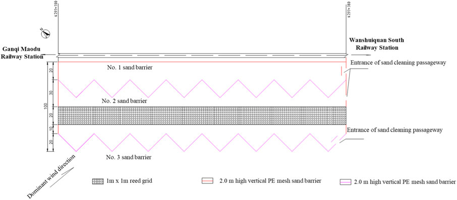
Figure 1. Arrangement method of sand mitigation measures.
As shown in Figure 2, a sand area environmental perception analyzer is arranged at a vertical distance of 100 m from the line at the test section K297 + 650. It monitors on-site sand environment parameters such as wind direction, wind speed, sand flow density, humidity, sunlight radiation, etc., and uploads the data to the online data management system in real time. This paper focuses on the wind speed, wind direction, and sand flow density data from 20 August 2022, to 2 July 2023, within a range of 0–4 m from the ground, to provide basic parameters for the calculation of sand accumulation in sand mitigation measures.
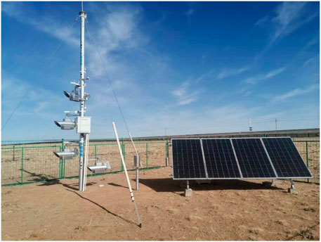
Figure 2. Wind and sand zone environmental perception analysis instrument.
Through the field observation and the existing empirical model analysis, the sand-starting wind speed is determined to be 8 m/s, that is, when the environmental wind speed exceeds 8 m/s, the sand particles on the ground will roll and saltate (Kok et al., 2012). Figure 3 is a wind speed and direction rose diagram in different seasons of the test section, where the maximum wind velocity per month is also given. The wind speed and direction data greater than the sand-starting wind speed are counted in the figure, and the data with wind speed less than 8 m/s are listed as “calm wind”. The frequencies of quiet wind in spring, summer, autumn and winter were 77.8%, 87.5%, 87.0% and 72.6%, respectively. Among them, the dominant wind direction in spring and autumn is due west; the dominant wind direction in autumn and winter is southwest. The frequency of wind speeds greater than the sand-starting wind speed is higher in spring and winter, at 22.2% and 27.4% respectively; the frequency of wind speeds greater than the sand-starting wind speed is slightly lower in summer and autumn, at 12.5% and 13% respectively. There are a total of 69 days in the year with wind speeds greater than the sand-starting wind speed, the average wind speed is 12 m/s, and the maximum wind speed occurred on 11 May 2023, at 26.4 m/s.
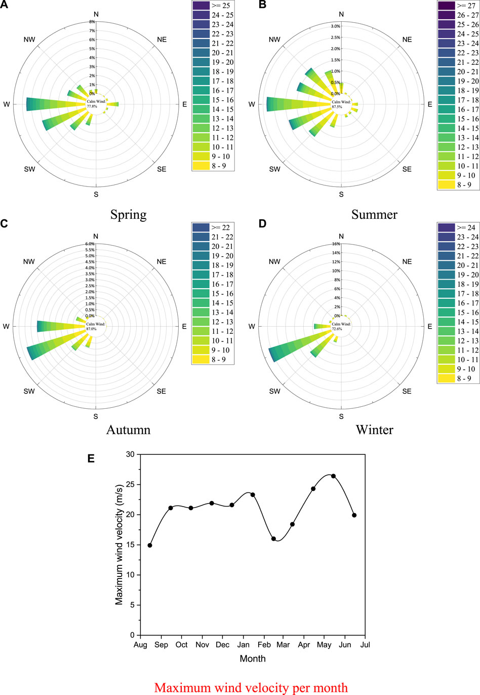
Figure 3. Wind speed, wind direction rose diagram for different seasons in the experimental sections: (A) Spring; (B) Summer; (C) Autumn; (D) Winter; (E) Maximum wind velocity.
Some monitoring data of the online wind-sand flow monitoring system can monitor the real-time wind speed and wind-sand flow density at different heights in real time. Here, wind-sand flow refers to the movement and behavior of sand particles driven by wind forces. The wind-sand flow density is defined as the mass of sand contained in the unit volume of air flow. The wind-sand area environmental perception analyzer has a built-in sand collection entrance of a specific area and is equipped with a weight sensor. Combined with the monitored wind speed, the wind-sand flow density at a specific height can be obtained. Due to the design limitations of the monitoring device, we were unable to monitor the wind-sand flow density in areas below 0.5 m. The structure of the wind-sand flow changes exponentially with height, and the wind-sand flow density near the ground is larger, so the actual wind-sand flow density may be under-estimated to a certain extent. The wind-sand flow density measured at different heights is shown in Figure 4. This monitoring result shows the typical characteristics of the wind-sand flow structure, that is, as the elevation increases, the wind-sand flow density rapidly decreases, showing an exponential decay rule. When the height from the ground is greater than 3 m, the measured wind-sand flow density is almost 0. Observations of the material collected in the sand collection box located at the 2 m position found that: there are fewer sand particles in the collected solid material, and the sand collection box is mainly composed of broken roots and seeds of sea buckthorn. Their density is much smaller compared to sand particles, easy to be blown away by the airflow, and has a small impact on the railway. Therefore, in numerical calculations, we choose a height of 2 m from the ground as the distribution range of the wind-sand flow. Through numerical averaging, the overall average wind-sand flow density is obtained as 3.50 × 10⁻⁵ kg/m3.
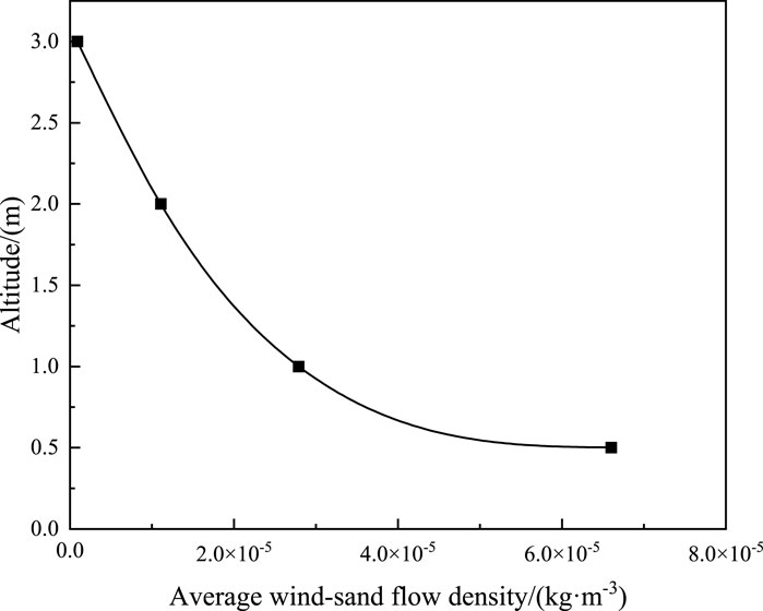
Figure 4. Wind-blown sand density at different heights.
The process of wind blowing sand is simulated by CFD technology using the Euler-Euler two-phase flow model. This model treats both wind and sand particles as continuous phases (Gidaspow, 1986). The control equations that need to be considered during calculation mainly include the mass conservation equation (continuity equation) and the momentum conservation equation. For the numerical simulation of wind-sand two-phase flow, the temperature exchange process between sand particles and air is usually not considered, so this model does not involve the energy conservation equation. In the Euler two-phase flow model, the spatial occupancy rate of the sand particle phase in the calculation domain is expressed by the volume fraction. The speed of the air phase is small and can be regarded as an incompressible fluid, so it satisfies the conditions for using the Navier-Stokes equation describing viscous incompressible fluid. The general form of its continuity equation is shown in Eq. 1 (Ferziger et al., 2020).
where
The momentum equation of the sand particle phase is shown in Eq. 2:
where
In this model, the gravity subject to the air phase is ignored, so the momentum equation of the air phase is shown in Eq. 3:
where
When solving turbulent motion, the Reynolds stress term in the Reynolds equation group is unknown, so the Reynolds equation group is not closed, and a turbulence model needs to be used to describe complex turbulent phenomena. The standard k-ε model introduces two independent transport equations (turbulent kinetic energy k and turbulent dissipation rate ε) to achieve closure of the Reynolds stress term. It is a widely used turbulence model that can handle various complex turbulence problems. In the Euler two-phase flow model, ignoring the compression of the air phase and the influence of the source term on the turbulence equation, the corresponding Eqs 4, 5:
(1) Turbulent kinetic energy equation:
(2) Turbulent dissipation rate equation:
where

Table 1. Model parameters of the standard k-ε model.
The sand particles are subjected to gravity, pressure gradient force and drag force. In the simulation of wind-sand two-phase flow, drag force can often be described by Syamlal-O'Brien model (O’Brien and Syamlal, 1993), which takes into account the influence of the volume fraction of sand particles on drag force. The larger the volume fraction of sand particles is, the more significant the interaction between particles will be, and the greater the drag force the particles will be subjected to. The formula of drag force f given by Syamlal-O'Brien model is as follows in Eq. 6:
where
The drag function is Eq. 7:
The functional relation of the relative Reynolds number is Eq. 8:
where
Free settling coefficient of solid is Eq. 9:
where
As shown in Figure 5, a reasonable calculation domain size was determined through gridless simulation. The final two-dimensional calculation domain is 200 m long and 23 m high. The upright sand barrier close to the embankment is 2 m high, the other two sand barriers are 1.5 m high, and the grass grid is 0.2 m high, with a length and width of 1 m each. The size of the numerical simulation model is set entirely according to the measured size on site, satisfying similarity at the geometric level. Due to the complex structure of the sand mitigation measures, it is necessary to simplify the calculation model. The zigzag sand barrier is equivalent to a straight line type, and the position is set at the midpoint of the zigzag sand barrier; the road cut is simplified to a trapezoidal rigid body; the upright sand barrier is simplified to a rigid body with a certain thickness and a porosity rate of 40%.
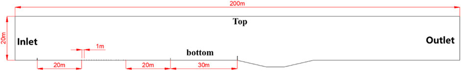
Figure 5. Boundary names and dimensions of the numerical model.
Due to the micro-geometric size features in the porous sand barrier and grass grid in the calculation domain, it is difficult to divide the structured grid in the calculation domain, so the meshing module in Ansys Workbench software is used to divide the unstructured grid in the calculation domain. The volume growth rate of the grid is 1.1. Local grid encryption technology is applied near the sand barrier and grass grid. In order to improve the overall grid quality and ensure the stability of the calculation, no boundary layer grid is divided near the ground. Finally, 130,000 unstructured grids were divided, the average grid quality was 0.88, and the aspect ratio was 1.18. The grid division situation is shown in Figure 6.
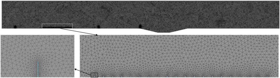
Figure 6. Schematic diagram of the mesh division and local refinement in the numerical model.
To ensure the applicability and accuracy of the model, it is necessary to set appropriate boundary conditions for the calculation domain. The wind-sand flow in reality is a very complex physical phenomenon. The wind speed and wind-sand flow density are significantly different at different time periods, and there is a certain correlation between the wind-sand flow density and wind speed. It is very difficult to fully simulate this phenomenon. Therefore, it is necessary to simplify it according to the existing computational fluid dynamics theory. In CFD simulation, we simplify the wind-sand flow into a steady flow that blows into the calculation domain at a constant wind speed and constant wind-sand flow density. The inlet is set as a velocity inlet boundary, and it is set in Eq. 10:
where
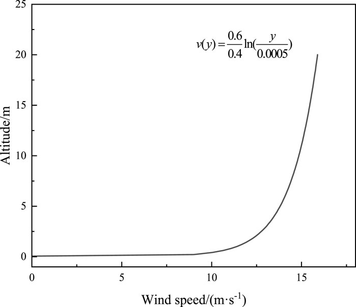
Figure 7. Wind speed profile at the velocity inlet.
The boundary condition of the outlet on the right is set as a free Out flow boundary, that is,
Table 2 shows the model parameters used in the numerical simulation model. The particle size and density of the sand particles are measured according to the sieving method and specific gravity bottle method in the “Geotechnical Test Method Standard”. Analysis of environmental monitoring data found that when the height from the ground is greater than 2 m, the measured wind-sand flow density is almost 0. Therefore, in the numerical simulation experiment, the sand particle phase is only blown in within 2 m from the ground at a volume fraction of 0.02%, and the speed of the sand particles (
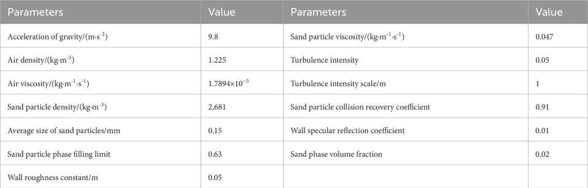
Table 2. Model parameter values in the computation.
The wall roughness constant/m is 0.05. This numerical simulation experiment uses the Phase Coupled Simple method for pressure-velocity coupled iteration. To ensure the accuracy of the calculation, the pressure uses second-order accuracy; the interpolation methods of momentum, turbulent kinetic energy, and turbulent dissipation rate use the Second Order Upwind; the volume fraction uses the high-order Quick format. At the same time, relaxation factors are set for each solution parameter, and it is considered to converge when the iterative residual drops below 10–5. The entire simulation process calculates a total of 40 s, the time step is 0.002 s, and each time step iterates 20 times. In the calculation process, the volume fraction of sand particles is set to 0 in the first 10 s, that is, only wind is blown into the calculation domain; in the last 30 s, the sand particle phase enters the calculation domain at a volume fraction of 0.02. The purpose is to make the flow field distribution of the entire calculation domain uniform before the sand particles are added, thereby improving the stability and accuracy of the calculation.
Figure 8 is a time-varying flow field and time-varying sand accumulation distribution cloud map in the calculation domain. The calculation time of 10 s corresponds to the state of the calculation domain without sand particles and the wind field reaching stability. When the airflow passes through the sand barrier, it is squeezed at the top and separated, forming a shear layer. The pressure difference on both sides of the shear layer makes the streamline become a downward inclined straight line. The upper part of the sand barrier is a blunt body with a sharp edge, and the boundary layer separates when the airflow passes through; therefore, the airflow above the sand barrier after the sand barrier forms a vortex and becomes a faster turbulence; the airflow below is slower, preventing the sand barrier After the sand accumulation is re-sanded. Because the sand barrier is a porous sand barrier, the airflow can pass through the pores of the sand barrier, so no obvious backflow phenomenon is found after the sand barrier. But as more sand particles enter the calculation domain, the streamline gradually concaves, and the inflection point of the streamline eventually coincides with the ground at the first grass grid.
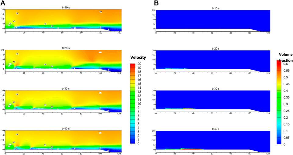
Figure 8. Time-varying flow field and time-varying sand accumulation distribution within the computational domain: (A) Velocity; (B) Volume fraction.
From the sand accumulation distribution map, it can be found that as the sand entering the calculation domain gradually increases, the sand accumulation after the first sand barrier in the sand mitigation measures gradually increases, and gradually spreads to the inside of the grass grid, but the spread speed is very slow, until the entire calculation time ends, the sand accumulation has not reached the second sand barrier.
Figure 9 is the velocity cloud map of the sand particle phase in the calculation domain, and the movement law of the wind-blown sand flow can be visually seen. When the wind-blown sand flow passes through the first sand barrier, part of it is blocked by the first sand barrier, and the other part of the sand particles are thrown to a higher position or directly through the pores of the sand barrier, and fall behind the sand barrier. The grass grid behind the barrier can play a fixed role in sand accumulation, so the sand velocity corresponding to the grass grid position in Figure 10 is almost 0. However, with the passage of time, the accumulation of sand behind the barrier continues to increase, and spreads to the last two sand barriers, and a secondary sand phenomenon appears. At this point, the last sand barrier will throw the wind flow into the air, so that it directly across the cutting, channeling to the other side of the line, will not affect the line.
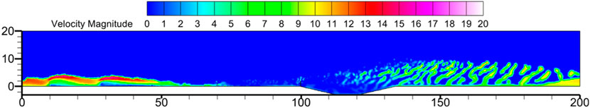
Figure 9. Velocity contour map in the computational domain under stable conditions.
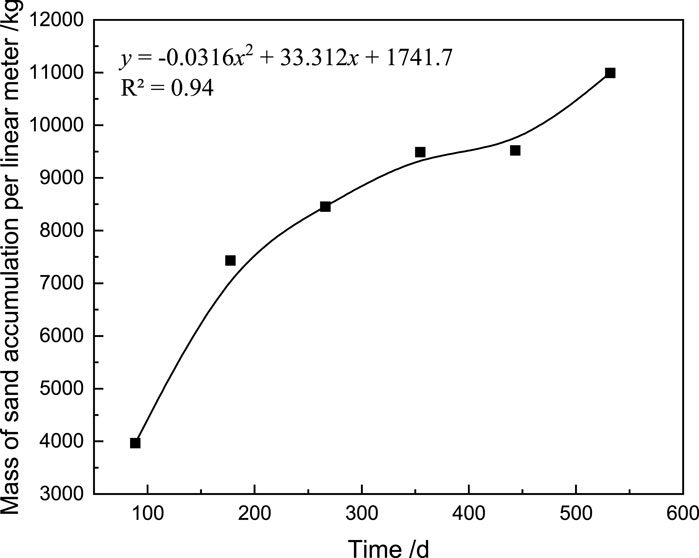
Figure 10. Variation of sand accumulation mass per meter over time.
The latter two sand barriers are located outside the protective distance of the first sand barrier, mainly to deal with the secondary sand formation outside the protective distance of the first sand barrier. In the case of extreme weather and serious secondary sand formation, the latter two sand barriers can play a very good protective effect. All in all, this not only avoids the impact of sand on the line, but also reduces the sand clearing cost caused by the accumulation of sand near the sand barrier.
Since the blown sand flow density of the actual project site is relatively discrete and cannot be directly used, the instantaneous blown sand flow density curve monitored on site in the test section from 20 August 2022. to 2 July 2023, and the actual accumulated sand in the sand box are calculated in this paper., and the measured average blown sand flow density is calculated as 3.5 × 10⁻⁵ kg/m3. In the numerical calculation model, the sand particles are stably input in the form of wind velocity contour and according to a certain volume fraction, and the total sediment transport time is 30 s. In order to normalize the actual sediment transport amount and the sediment transport amount of the numerical calculation model, it is necessary to make some corrections to obtain the actual sediment transport time corresponding to the numerical calculation model (as shown in Eq. 12):
where
The calculation results select the sand accumulation cloud maps at 5 s, 10 s, 15 s, 20 s, 25 s, and 30 s. Then, using Tecplot post-processing software, the spatial distribution of the sand accumulation volume fraction behind the sand barrier corresponding to each time is analyzed to obtain the sand accumulation amount and sand accumulation width. A mathematical formula is used to fit this curve, and a preliminary relationship equation between the sand accumulation amount, sand accumulation width, and set calculation time is obtained, as shown in Figures 10, 11.
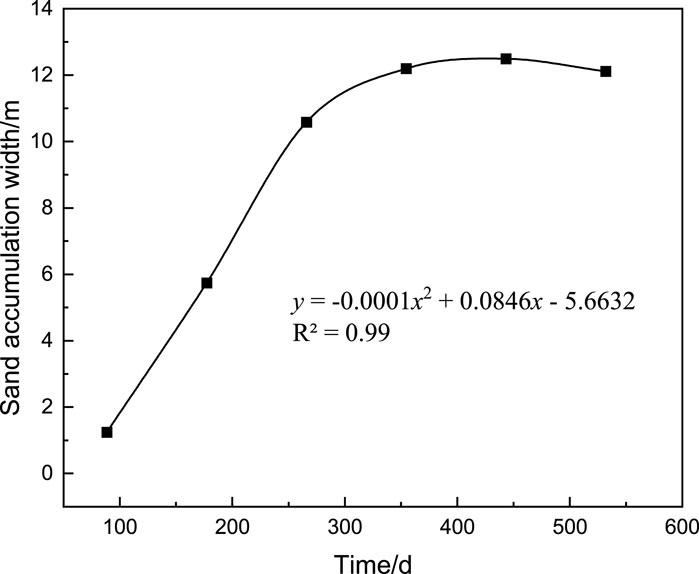
Figure 11. Variation of sand accumulation width within the sand mitigation measures over time.
According to the relationship equation obtained between the sand accumulation amount, sand accumulation width, and time, it can be seen that in the first 350 days, the sand accumulation width and sand accumulation mass in the entire sand mitigation measure are in a state of rapid rise; in the range of 350 days–450 days, the sand accumulation mass and sand accumulation width in the sand mitigation measurement are in a state of slow increase, indicating that the sand accumulation in the sand mitigation measurement has sufficient height at this time, and most of the sand particles can cross the sand barrier and be thrown into the air; but after 450 days, the sand accumulation width in the sand mitigation measurement remains almost unchanged, while the sand accumulation mass significantly increases, indicating that all the grass grids in the sand mitigation measurement have been filled at this time, the height of sand accumulation continues to increase, and when the height of sand accumulation exceeds the sand fixing ability of the grass grid, the sand accumulation in the sand mitigation measurement will become a new source of sand, and its secondary sanding phenomenon will affect the road cut section. Therefore, the appropriate time for sand cleaning is between 350 days and 450 days.
This study provides a comprehensive analysis of wind-blown sand accumulation along the Ganquan Railway through on-site monitoring and numerical simulations using Computational Fluid Dynamics (CFD). The key findings are as follows:
(1) The dominant wind direction in the Ganquan Railway test section is due west during spring and winter, and southwest during autumn and winter. The average wind speed is 12 m/s. The wind-sand flow structure is predominantly distributed within 2 m from the ground, with an average wind-sand flow density of 3.5 × 10⁻⁵ kg/m³.
(2) In the absence of sand accumulation, the streamline of the wind field in the calculation domain is a downward inclined straight line. As sand accumulates behind the sand barriers, the topography and geomorphology of the area change, causing the wind field streamline to gradually become concave. The inflection point of the streamline eventually coincides with the ground at the first grass grid.
(3) The width of sand accumulation in the test section initially increases uniformly before stabilizing. The mass of sand accumulation, however, rises uniformly to a plateau and then increases rapidly with time. The optimal time for sand cleaning is between the 350th and 450th days after the sand barrier is implemented.
(4) This study integrates field data with CFD simulations to provide a more accurate and comprehensive understanding of wind-sand dynamics, which enhances the reliability of sand accumulation predictions. By analyzing the temporal evolution of sand accumulation, the study identifies an optimal timeframe for sand removal, which can significantly improve maintenance efficiency and reduce operational costs. The methodology and findings can be applied to other engineering projects facing similar sand accumulation challenges.
The raw data supporting the conclusions of this article will be made available by the authors, without undue reservation.
SH: Conceptualization, Data curation, Formal Analysis, Funding acquisition, Validation, Visualization, Writing–original draft. TaM: Investigation, Software, Writing–original draft. FJ: Software, Supervision, Writing–original draft. FN: Methodology, Resources, Validation, Writing–original draft. XW: Funding acquisition, Project administration, Writing–original draft. TiM: Conceptualization, Methodology, Project administration, Supervision, Validation, Writing–review and editing.
The author(s) declare that financial support was received for the research, authorship, and/or publication of this article. This research was funded by Major research project of China Railway Engineering Design Consulting Group Co., LTD. (Research 2022-3); Key Topics of Ganquan Railway Co., LTD. (GJNY-21-68).
The authors also thank the reviewers for their comments on this manuscript.
Authors SH, TaM, and FJ were employed by China Railway Engineering Consulting Group Co., Ltd.
Authors FN and XW were employed by Guoneng Ganquan Railway Group Co., Ltd.
The remaining author declares that the research was conducted in the absence of any commercial or financial relationships that could be construed as a potential conflict of interest.
All claims expressed in this article are solely those of the authors and do not necessarily represent those of their affiliated organizations, or those of the publisher, the editors and the reviewers. Any product that may be evaluated in this article, or claim that may be made by its manufacturer, is not guaranteed or endorsed by the publisher.
Ahmadzadeh, E., Samadianfard, S., Xiao, Y., and Toufigh, V. (2024). Feasibility of micro-organisms in soil bioremediation and dust control. Biogeotechnics 2, 100085. doi:10.1016/j.bgtech.2024.100085
An, L., Che, H., Xue, M., Zhang, T., Wang, H., Wang, Y., et al. (2018). Temporal and spatial variations in sand and dust storm events in East Asia from 2007 to 2016: relationships with surface conditions and climate change. Sci. Total Environ. 633, 452–462. doi:10.1016/j.scitotenv.2018.03.068
Andrea Lo, G., Roberto, N., Luigi, P., and Nicolas, C. (2019). Wind-blown particulate transport: a review of computational fluid dynamics models. Math. Eng. 1, 508–547. doi:10.3934/mine.2019.3.508
Bruno, L., Fransos, D., and Lo Giudice, A. (2018a). Solid barriers for windblown sand mitigation: aerodynamic behavior and conceptual design guidelines. J. Wind Eng. Industrial Aerodynamics 173, 79–90. doi:10.1016/j.jweia.2017.12.005
Bruno, L., Horvat, M., and Raffaele, L. (2018b). Windblown sand along railway infrastructures: a review of challenges and mitigation measures. J. Wind Eng. Industrial Aerodynamics 177, 340–365. doi:10.1016/j.jweia.2018.04.021
Dong, Z. B., Luo, W., Qian, G., and Wang, H. T. (2011). Evaluating the optimal porosity of fences for reducing wind erosion. Sci. Cold Arid Regions 3, 1–12. doi:10.3724/SP.J.1226.2011.00001
Horvat, M., Bruno, L., and Khris, S. (2022). Receiver Sand Mitigation Measures along railways: CWE-based conceptual design and preliminary performance assessment. J. Wind Eng. Industrial Aerodynamics 228, 105109. doi:10.1016/j.jweia.2022.105109
Horvat, M., Bruno, L., Khris, S., and Raffaele, L. (2020). Aerodynamic shape optimization of barriers for windblown sand mitigation using CFD analysis. J. Wind Eng. Industrial Aerodynamics 197, 104058. doi:10.1016/j.jweia.2019.104058
Kok, J. F., Parteli, E. J. R., Michaels, T. I., and Karam, D. B. (2012). The physics of wind-blown sand and dust. Rep. Prog. Phys. 75, 106901. doi:10.1088/0034-4885/75/10/106901
Lima, I. A., Parteli, E. J. R., Shao, Y., Andrade, J. S., Herrmann, H. J., and Araújo, A. D. (2020). CFD simulation of the wind field over a terrain with sand fences: critical spacing for the wind shear velocity. Aeolian Res. 43, 100574. doi:10.1016/j.aeolia.2020.100574
Lo Giudice, A., and Preziosi, L. (2020). A fully Eulerian multiphase model of windblown sand coupled with morphodynamic evolution: erosion, transport, deposition, and avalanching. Appl. Math. Model. 79, 68–84. doi:10.1016/j.apm.2019.07.060
Luca, B., Coste, N., Fransos, D., Lo Giudice, A., Preziosi, L., and Raffaele, L. (2018). Shield for sand: an innovative barrier for windblown sand mitigation. Recent Patents on engineering 12, 237–246. doi:10.2174/1872212112666180309151818
Luo, X., Li, J., Tang, G., Li, Y., Wang, R., Han, Z., et al. (2023). Interference effect of configuration parameters of vertical sand-obstacles on near-surface sand transport. Front. Environ. Sci. 11. doi:10.3389/fenvs.2023.1215890
Miao, L., Wang, H., Sun, X., Wu, L., and Fan, G. (2024). Effect analysis of biomineralization for solidifying desert sands. Biogeotechnics 2, 100065. doi:10.1016/j.bgtech.2023.100065
O’brien, T. J., and Syamlal, M. (1993). “Particle cluster effects in the numerical simulation of a circulating fluidized bed,” in Proceeding of the Fourth International Conference on Circulating Fluidized Beds, Hidden Valley Conference Center and Mountain Resort Somerset, Pennsylvania, United States, 345–350.
Raffaele, L., Coste, N., and Glabeke, G. (2022). Life-cycle performance and cost analysis of sand mitigation measures: toward a hybrid experimental-computational approach. J. Struct. Eng. 148, 04022082. doi:10.1061/(asce)st.1943-541x.0003344
Raffaele, L., Van Beeck, J., and Bruno, L. (2021). Wind-sand tunnel testing of surface-mounted obstacles: similarity requirements and a case study on a Sand Mitigation Measure. J. Wind Eng. Industrial Aerodynamics 214, 104653. doi:10.1016/j.jweia.2021.104653
Ren, T., Gao, Y., Yuan, L., and Zhao, C. (2024). Robinia pseudoacacia sand stabilizer: its sand fixation effects and mechanical properties. Front. Environ. Sci. 12. doi:10.3389/fenvs.2024.1304830
Sherzad, M. F., and Goossens, D. (2022). Wind tunnel experiments and field observations of aeolian sand encroachment around vernacular settlements in the saharan and arabian deserts. Buildings 12, 2006. doi:10.3390/buildings12112006
Watson, A. (1985). The control of wind blown sand and moving dunes: a review of the methods of sand control in deserts, with observations from Saudi Arabia. Q. J. Eng. Geol. Hydrogeology 18, 237–252. doi:10.1144/gsl.qjeg.1985.018.03.05
Xin, G., Huang, N., Zhang, J., and Dun, H. (2021). Investigations into the design of sand control fence for Gobi buildings. Aeolian Res. 49, 100662. doi:10.1016/j.aeolia.2020.100662
Xin, G., Zhang, J., Fan, L., Deng, B., and Bu, W. (2023). Numerical simulations and wind tunnel experiments to optimize the parameters of the second sand fence and prevent sand accumulation on the subgrade of a desert railway. Sustainability 15, 12761. doi:10.3390/su151712761
Zhang, K., Tian, J., Qu, J., Zhao, L., and Li, S. (2022a). Sheltering effect of punched steel plate sand fences for controlling blown sand hazards along the Golmud-Korla Railway: field observation and numerical simulation studies. J. Arid Land 14, 604–619. doi:10.1007/s40333-022-0019-7
Zhang, K., Zhao, L.-M., Zhang, H.-L., Guo, A.-J., Yang, B., and Li, S. (2022b). Numerical simulation on flow field, wind erosion and sand sedimentation patterns over railway subgrades. J. Mt. Sci. 19, 2968–2986. doi:10.1007/s11629-022-7396-4
Keywords: windblown sand, environmental monitoring, Euler two-phase flow model, sand accumulation calculation, railway infrastructures
Citation: Huang S, Ma T, Jiang F, Nie F, Wang X and Ma T (2024) Numerical simulation and field study on predicting wind-blown sand accumulation in sand mitigation measures of the Ganquan railway. Front. Earth Sci. 12:1443030. doi: 10.3389/feart.2024.1443030
Received: 03 June 2024; Accepted: 27 June 2024;
Published: 16 July 2024.
Edited by:
Ran An, University of Bristol, United KingdomReviewed by:
Chuanqin Yao, Shanghai Normal University, ChinaCopyright © 2024 Huang, Ma, Jiang, Nie, Wang and Ma. This is an open-access article distributed under the terms of the Creative Commons Attribution License (CC BY). The use, distribution or reproduction in other forums is permitted, provided the original author(s) and the copyright owner(s) are credited and that the original publication in this journal is cited, in accordance with accepted academic practice. No use, distribution or reproduction is permitted which does not comply with these terms.
*Correspondence: Tiantian Ma, dHRtYUB3aHJzbS5hYy5jbg==
Disclaimer: All claims expressed in this article are solely those of the authors and do not necessarily represent those of their affiliated organizations, or those of the publisher, the editors and the reviewers. Any product that may be evaluated in this article or claim that may be made by its manufacturer is not guaranteed or endorsed by the publisher.
Research integrity at Frontiers
Learn more about the work of our research integrity team to safeguard the quality of each article we publish.