 Salvatore de Lorenzo
 Maddalena Michele
- 1Dipartimento di Scienze della Terra e Geoambientali, Università di Bari “Aldo Moro”, Bari, Italy
- 2Istituto Nazionale di Geofisica e Vulcanologia, Roma, Italy
Circular crack models with a constant rupture velocity struggle to effectively model both the amplitude and duration of first P-wave pulses generated by small magnitude seismic events. Assuming a constant rupture velocity is unphysical, necessitating a deceleration phase in the rupture velocity to uphold the causality of the healing process. Moreover, a comprehensive failure model might encompass an initial nucleation phase, typically characterized by an increase of the initial rupture velocity. Studies have demonstrated that quasi-dynamic circular crack models featuring variable rupture velocities can accurately model the shape of the observed first P-wave pulse. Based on these principles, an Empirical Green’s function (EGF) approach was previously formulated to estimate the source parameters of small magnitude earthquakes, called MAIN. In addition to determine the source radius and stress drop, this method also enables the inference of the temporal evolution of rupture velocity. However, this method encounters difficulties when the noise-to-signal ratio in the recordings of smaller earthquakes used as EGF exceeds 5%, a common situation when employing regional-scale recordings of small-magnitude earthquakes as EGF. Through synthetic tests, we demonstrated that, in such instances, the problem of this technique is that the alignment between the onset of P waves of EGF and MAIN is not rightly recovered after the initial inversion step. Consequently, a novel inversion method has been developed to address this issue, enabling the identification of the optimal alignment of P-wave arrivals in EGF and MAIN across all stations. A Bayesian statistical approach is proposed to meticulously investigate the solutions of model parameters and their correlations. Using the new technique on a small magnitude earthquake (ML = 3.3) occurred in Central Italy enabled us to identify the most likely rupture models and examine the issue of correlation among model parameters. Application of Occam’s Razor Principle suggests that, for the investigated event, a circular crack model should be favored over a heterogeneous rupture model.
1 Introduction
When an earthquake occurs, the available energy is partitioned between the radiated energy and the fracture energy (i.e., the energy lost to the heating and plastic deformation accompanying the rupture growth) (Madariaga, 1976). Depending primarily on the frictional forces along the fault, the rupture may then grow at low or high rupture velocity. The slower the rupture velocity Vr, the less available energy is radiated (Boatwright, 1980). Moreover, the changes in rupture velocity are responsible for the high-frequency damaging waves (Madariaga, 1977). Thus, rupture velocity and its evolution are crucial parameters for understanding earthquake physics and assessing seismic hazard in a tectonic region.
In studies aimed at inferring the source parameters from the inversion of seismic spectra, rupture velocity is generally assumed to be less than the shear wave velocity VS. However, numerous recent studies suggest that assuming a sub-shear rupture velocity regime (Vr < VS) may be incorrect. Indeed, many large magnitude earthquakes are characterized by a super-shear rupture velocity regime (e.g., Bouchon and Vallée, 2003; Wang et al., 2016; Chounet et al., 2018).
As concerns the small magnitude earthquakes, a minor number of studies have been dedicated to accurately estimating the rupture velocity. In these cases, in fact, the correlation among source parameters may strongly bias the obtained results (see Abercrombie, 2021 for an overview of the challenges related to source parameter estimation). Therefore, it is crucial to further develop methods aimed at precisely determining the rupture velocity of small magnitude earthquakes. Since a kinematic circular crack model rupturing at a constant velocity may yield biased estimates of rupture velocity, stress drop and source dimension, owing to their correlation (Deichmann, 1997; Chounet et al., 2018; Abercrombie, 2021), it is essential to investigate whether the use of quasi-dynamic circular crack models with variable rupture velocity can assist in better constraining these parameters. Including a variable rupture velocity has indeed been shown to be necessary to effectively model both the rupture duration and amplitude of the first P-pulses of small magnitude earthquakes, a task where constant rupture velocity models are insufficient (Deichmann, 1997). Furthermore, while correlations among model parameters may be inevitable when using earthquake recordings from only one or few stations, it is expected that these tradeoffs can be reasonably mitigated when a larger number of recordings, covering various azimuths and distances, are included. The worldwide increase in the availability of high-quality recordings of small earthquakes at a regional scale now provides the opportunity to assess whether quasi-dynamic circular crack models can accurately reproduce the main properties of the energy radiated by a small magnitude earthquake.
Based on these grounds, in this article we propose an improvement of a previously developed technique (de Lorenzo et al., 2008 in the next referred to as DFB) designed to deduce the source parameters of a small magnitude earthquake. The technique assumes that the rupture follows the quasi-dynamic behavior of the Sato (1994) model. The new formulation of the inverse method allows to use also seismic recordings characterized by a noise-to-signal ratio greater than 10%, as it is commonly observed on low-pass filtered traces of seismic recordings of small earthquakes (ML < 2) recorded at a regional scale (source-to-receiver distances less than 100 km).
2 Materials and methods
In this section, we begin by outlining the theoretical basis of the circular crack model considered in this study. Subsequently, we provide a concise overview of the inversion method introduced by DFB, followed by an explanation, illustrated through a synthetic test, of the necessity for modifying this method. Finally, we describe the new technique for inferring source model parameters.
2.1 Kinematic and quasi-dynamic source models
The representation theorem (Aki and Richards, 2002) constitutes the general form of the equations describing the displacement at a point inside an elastic medium, due to the forces acting in a source volume. It shows that the content of a seismic recording is described by two tensors. The first one is the Green’s tensor, i.e., the response of the medium to impulsive point forces located at the hypocenter of the earthquake. The second one is the seismic moment tensor, that describes the complex system of body forces acting in the source volume. The aim of seismic source studies is therefore reconducted to infer the shape of the source time function, i.e., the moment rate function
where the integral is computed on the ruptured surface
In the kinematic rupture models the slip function is prescribed on the fault. Simple kinematic circular crack models with a constant stress on fault and rupturing at a constant rupture velocity (e.g., Brune, 1970) are considered unable to furnish reliable estimates of source parameters (Abercrombie, 2021). There are several possible explanations for this disagreement, such as the heterogeneity of the friction on the fault plane and/or the non-circular geometry of the final ruptured area. However, another less considered explanation is that the kinematic models do not account for the evolution of the rupture velocity during the rupture process (e.g., Deichmann, 1997; Madariaga and Ruiz, 2016).
The first simple but complete kinematic model, consisting of a circular crack rupturing at a constant velocity, was proposed by Sato and Hirasawa (1973). This model reproduces the general properties of the waves radiated during an earthquake, such as focusing, directivity and stopping phases (e.g., Madariaga, 2007). According to Boatwright (1980), the Sato and Hirasawa (1973) circular crack is a quasi-dynamic model, in that the slip function complies at each time with the theoretical solution to the static problem of a circular crack (Eshelby, 1957). From a theoretical point of view, the main limit of this model is represented by the instantaneous non-causal freezing of the rupture once the rupture front reaches the border of the circular fault (Madariaga, 2007). To evaluate what happens in the interior of the fault when the rupture stops, it was then necessary to solve the dynamical problem. The solution to this problem was found by Madariaga (1976). He demonstrated that, when the rupture reaches the border, the rim of the fault generates P, S and Rayleigh healing waves that propagate inward from the border. The passage of these waves progressively reduces to zero slip rate in the interior of the fault allowing a causal healing of the rupture.
Based on these findings, Boatwright (1980) developed two quasi-dynamic models aimed at overcoming the limit of the Sato and Hirasawa (1973) model. These two models enclose into an analytical formulation the continuous decrease of the slip-rate on the fault. In the first one, known as the decelerating D-model, an initial constant rupture speed propagation phase is followed by a linear decrease to zero of rupture velocity, leading to a progressive decrease of slip rate on the fault (Figure 2 of Boatwright, 1980). The second one is the M-model, which is a simplified analytic representation of the slip rate evolution discovered by Madariaga (1976). The M-model exhibits a similar trend, with a more pronounced decrease in slip rate after the rupture stops (Figure 3 of Boatwright, 1980).
Quasi-dynamic analytical models that include variations in rupture velocity play a crucial role in formulating models for estimating source parameters from the inversion of P and/or S waveforms observed during seismic radiation. These models use closed analytical forms of the slip function, enabling simpler numerical schemes compared to the finite difference solutions used in dynamic problem simulations. The most complete analytical model of circular crack was proposed by Sato (1994), which incorporated the decelerating phase introduced by Boatwright (1980) into a three-stage rupture velocity history. In the Sato (1994) model, the rupture velocity initially increases to simulate the low moment rate nucleation phase (e.g., Ellsworth and Beroza, 1998). This acceleration phase is followed by a constant rupture velocity phase and then by a final linear decrease to zero of rupture velocity (Vr), according to Boatwright (1980) D-model (see Figure 1).
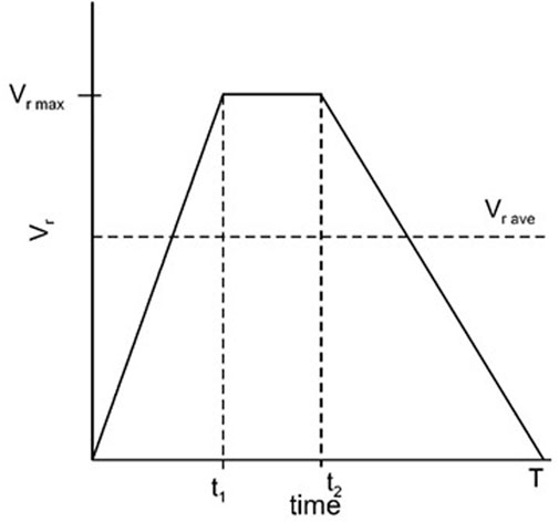
Figure 1. Plot of the rupture velocity history considered in this article. The nucleation phase corresponds to the initial accelerating phase from 0 and t1; the decelerating phase occurs from t2 and T.
The analytical expressions of the AMRF found by Sato (1994) is:
where
In this expression, L is the radius of the final crack,
In Eq. 4 Vrave is the average rupture velocity. As shown in DFB, the expression of AMRF for P-waves holds in all the subsonic regime, i.e.,
2.2 The limits of the starting EGF technique
One of the most used methods for inferring the AMRF of an earthquake is the Empirical Green’s Function (EGF) method (Hartzell, 1978). This method involves approximating the Green’s function with the recording of a small magnitude earthquake, referred to as the EGF, which is co-located with the earthquake of interest and has the same focal mechanism. In the original EGF method the AMRF is estimated by dividing the spectrum of the MAIN by the spectrum of the EGF. To mitigate the numerical instability caused by spectral division, the first improvement to the original technique was the use of a water-level criterion (e.g., Mueller, 1985). Recent advancements in this technique (e.g., Bertero et al., 1997; Vallée, 2004) have introduced positivity constraints and the conservation of seismic moment, further reducing the instability associated with spectral division.
To address the instability issues associated with spectral deconvolution an alternative EGF approach, based on convolution rather than deconvolution, was also developed (e.g., Zollo et al., 1995; Shibazaki et al., 2002). This approach involves assuming the functional form of the AMRF and formulating an inverse problem for the inference of the AMRF model parameters.
As concerns small magnitude earthquakes, DFB developed a similar EGF technique, assuming the AMRF derived from the Sato (1994) model described earlier. They applied the technique to model the seismic radiation of some earthquakes of the 1997 Umbria-Marche seismic sequence, but using only high-quality recordings as EGF, i.e., seismograms of small magnitude earthquakes characterized by a noise-to-signal ratio less than 5%.
In this article, we aim to demonstrate how the inverse problem developed by DFB needs modification to enable the use of EGFs recorded at a regional scale (source-to-receiver distance less than 100 km), which typically have noise-to-signal ratios exceeding 10%. The new technique utilizes the same theoretical framework as the DFB method, which we will briefly summarize here.
Let us consider a mainshock (referred to as the MAIN) and a smaller magnitude earthquake recorded at M seismic stations:
where the symbol * indicates the time domain convolution and
The search for the optimal model parameters is performed using the Simplex Downhill method (Press et al., 1989), which is a highly efficient technique for exploring the model parameter space in nonlinear inverse problem, as shown also in other studies (e.g., Zollo and de Lorenzo, 2001 and references therein). The synthetic tests described in DFB suggest that the inversion method is robust and effective when dealing with data characterized by low noise N to signal S ratio (N/S less than 5%). The inversion scheme proposed by DFB is based on two steps:
In the initial step of the inversion process, a single-station inversion is performed at each available seismic station, allowing to estimate the best-fit model parameter vector for that station. Since the inversion is performed in the time domain, it is necessary to determine the optimal alignment between the onset of the first P-wave arrival of the Empirical Green’s Function (EGF) and the mainshock (MAIN), after both signals are filtered below the corner frequency of the EGF, as prescribed by the technique (Hartzell, 1978). However, due to the application of generally used non-causal low-pass filter, the onset of the filtered P-waves from both MAIN and EGF may become misaligned. Additionally, the onset of the P-wave in the EGF could be masked by noise due to the small size of the EGF. Moreover, the P-wave onset in the MAIN, particularly during the nucleation phase of the rupture process, may be gradually emergent, making it challenging to identify.
To address these challenges, DFB proposed conducting 2
In the second step of the DFB inversion, the joint inversion of EGF-MAIN pairs from all seismic stations is conducted, with each pair’s optimal alignment fixed at the value determined in the first step. Notably, the station estimates of model parameters obtained in the first step are disregarded in the second step of the DFB procedure. Due to the nonlinear nature of the equations linking model parameters and data, DFB employed the random deviates approach to estimate errors on model parameters. Through a robust analysis using synthetic and real EGF data, DFB demonstrated that the effectiveness of the inversion technique in recovering true model parameters is highly dependent on the level of noise in the data. When the noise-to-signal (N/S) ratio is less than 5%, stable estimates and reliable AMRF are obtained (Figure 5B of DFB). Conversely, when N/S ≥ 10%, multiple solutions are inferred (Figure 5C of DFB), resulting in a reduced resolution of the AMRF model parameters. The difficulties arise because, at higher noise levels (N/S ≥ 10%), the increased noise amplitude can introduce spurious oscillations around the first P-wave pulse of the EGF. When convoluted with the AMRF, these oscillations may produce theoretical signals that incorrectly align with the observed P-wave pulses. Therefore, DFB limited the application of this method to a small number (two or three) of MAIN-EGF pairs from select seismic events to mitigate these issues.
2.3 A synthetic test with a real noisy EGF
A robust synthetic study to evaluate the reliability of the results for the single station inversion (first step) has been already conducted in DFB, where both the effect of a different location of MAIN and EGF, the uncertainty in focal mechanisms and many other aspects were analyzed through synthetic tests. Obviously, those results remain still valid.
To elucidate the necessity for modifying the DFB inversion strategy in the presence of noisy waveforms (N/S ≥ 10%), we present the results of its application in two synthetic tests, using three-component recordings at the seismic station CSP1 of a small earthquake (ML = 1.9) occurred in Central Italy. The waveforms exhibit a low noise-to-signal ratio (N/S), as detailed in Table 1.
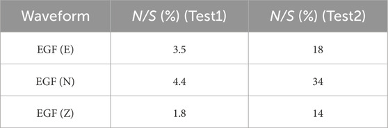
Table 1. Noise to signal ratio of EGF and MAIN for the two synthetic tests.
In test1, after the application of a low-pass filter to the EGF below the corner frequency (fc=10 Hz) we estimated a noise-to-signal ratio N/S ≤ 5% (Table 1). The observed synthetic mainshock was computed using Eq. 5 with the following model parameters:
The results of the first step of inversion are summarized in Figure 2A. All parameters are accurately recovered with minimal uncertainties, which could also be addressed using the random deviates technique, as discussed in DFB. It is worth to note that, in this case, the true alignment between the onset of P-waves of the MAIN and EGF is correctly identified after the inversion. In fact, the absolute minimum of the misfit function corresponds to this alignment (i.e., zero shift of the EGF relative to the MAIN).
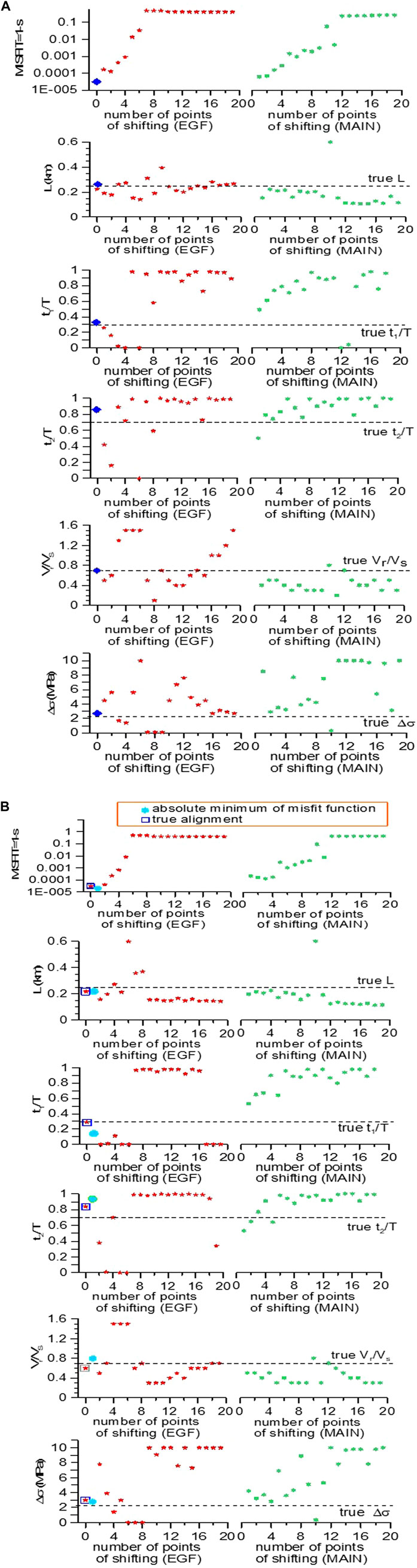
Figure 2. (A) Inversion results for test1. Red points represent the inversion results obtained by back shifting the EGF with respect to the initial alignment. Green points represent the inversion results obtained by back shifting the MAIN with respect to the initial alignment. The blue rhombus represents the solutions for the true alignment between the onset of the MAIN and the EGF, that, in this case, coincides with the best fit solution. (B) Inversion results for test2. Red points represent the inversion results obtained by back shifting the EGF with respect to the initial alignment. Green points represent the inversion results obtained by back shifting the MAIN with respect to the initial alignment. The blue rectangles represent the solutions for the true alignment between the onset of the MAIN and the EGF, that do not coincide, in this case, with the best fit solutions, represented by the cyan circles.
In test2, to simulate a scenario with a noisiest EGF, we added to the EGF a random noise obtained as a linear combination of random sinusoidal waves with frequencies
Using Eq. 7, the noise-to-signal ratio of the EGF was increased above 10%, as detailed in Table 1. The same model parameters of test1 (Eq. 6) were used to compute the observed synthetic mainshock. The results of the first step of inversion are depicted in Figure 2B. The source parameters exhibit slightly higher uncertainty compared to test 1, which can be mitigated using the random deviates technique as discussed in DFB. However, the most significant issue arises from the erroneous alignment between the onset of P-waves of the EGF and MAIN inferred from the inversion. We discuss in the next section the reason why this problem may severely impede to find the optimal model parameter solution when using the recordings of the EGF and MAIN at several stations. The excellent waveform fitting in both tests is illustrated in Figure 3, highlighting a strong a correlation among the source parameters that enables accurate reproduction of the observed seismogram even with small differences of the model parameters from their true values.

Figure 3. Matching between observed and theoretical synthetic waveforms for the two synthetic tests. Green lines represent the synthetic observed waveforms. Blue lines represent the synthetic retrieved waveforms.
2.4 The new formulation of the inverse problem
In the DFB inversion process, the second stage involves identifying the optimal model parameters by keeping the P-wave onset alignments of EGF and MAIN fixed at the values obtained in the first stage. However, when N/S ≥ 10%, the recovered alignments may be inaccurate, and combining these inaccuracies across multiple stations can hinder the search for the absolute minimum of the misfit function. This observation is not mere speculation; it derives from several trials we conducted using both synthetic and real data.
Therefore, the only feasible approach to proceed with the second stage of DFB inversion would be to conduct multiple inversions, each incorporating a different combination of alignments. Unfortunately, this problem exhibits exponential complexity. In fact, if Ms represents the number of stations, exploring all the possible combinations of alignments requires an enormous number
Based on these new findings, we have opted to replace the second step of the inversion process of DFB with an alternative approach, which is inspired by techniques used to reconstruct slip functions on faults for cases involving heterogeneous ruptures (e.g., Festa and Zollo, 2006). In such cases, solutions obtained from the first step of single station inversion are used to construct the final solution, whereas they were ignored in the DFB scheme.
In the new approach, we aim to assess which solution from the first inversion step best represents the source process. To do this, for each of the station solutions found at the first step we must first evaluate the misfit at the remaining stations. Given our observation that the optimal alignment between MAIN and EGF is unreliable with noisy seismograms (Figure 2B), we must compute the misfit function for every possible alignment of EGF-MAIN pairs at all other stations. In this way we can select the station solution that gives rise to the overall minimum misfit. From a computational point of view, we observe that, for each of the
Owing to the nonlinear form of the inverse problem, the uniqueness of the solution is however not guaranteed. A further exploration of the whole model parameter space is then required to find the model parameter solution which corresponds to the absolute minimum of the misfit function. This third and final step, moreover, is required also to analyze the correlation among model parameters that can result in multiple solutions. Instead of using the empirical approach based on random deviates, this step is now realized through a grid-search method, based on a modified Bayesian formulation of the inverse problem as proposed by Hu et al. (2008). The probability density function (pdf) of a model m given the measured data d,
where
Moreover, if a
The preliminary estimates are often derived from previous studies based on the assumption of a constant rupture velocity model. As a result, the preliminary information can be used only to define a range of admissible values for
where:
In Eq. 12
As concerns the pdf, Hu et al. (2008) showed that
In Eq. 13
Using Eq. 14, the above expression Eq. 8 becomes:
To account for the different level of noise on data at each station, M is computed as the weighted sum of the complementary semblances
through the equation:
In Eq. 16 si represent the single station semblances, whereas in Eq. 17 the weights are computed using the rule:
In Eq. 18 (N/S) Main, i and (N/S)EGF, I represent, respectively the noise-to-signal-ratio of Main and EGF. After inferring the most probable solution, a final test, based on the Occam Razor principle (Akaike, 1973), will be conducted to determine whether the source model obtained from the inversion of all the data is preferable to the heterogeneous source model inferred in the initial step.
3 Application to a real case
To show how the method works, we will analyze a pair of EGF-MAIN events that were recorded during the seismic sequence that occurred in the Central Italy in 2016. This sequence was initiated by a MW = 6 earthquake occurred on 24 August 2016 (Chiaraluce et al., 2017) and persisted for several months, generating over one hundred earthquakes daily (Michele et al., 2016; Chiaraluce et al., 2022). The MAIN (ML = 3.3) and EGF (ML = 1.9) events were located close to each other near the small town of Fiordimonte (MC). They represent a couple of double-difference relocated earthquakes (Waldhauser and Ellsworth, 2000) from the Michele et al. (2020) catalog. The absolute locations of the MAIN and the EGF were obtained from the CLASS catalog (Latorre et al., 2023), while the focal mechanism of MAIN, as reported by Malagnini and Munafò (2018), is summarized in Table 2 and shown in Figure 4. Both events exhibit similar focal mechanisms, which was evident from the coincidence of P-wave polarities observed at nearly all the stations.
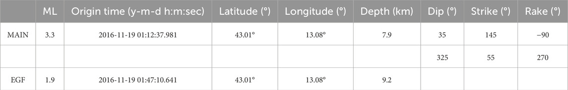
Table 2. Local magnitude, origin time and geographic coordinates of the hypocenter of MAIN and EGF. The focal mechanism solutions of the mainshock are also reported.
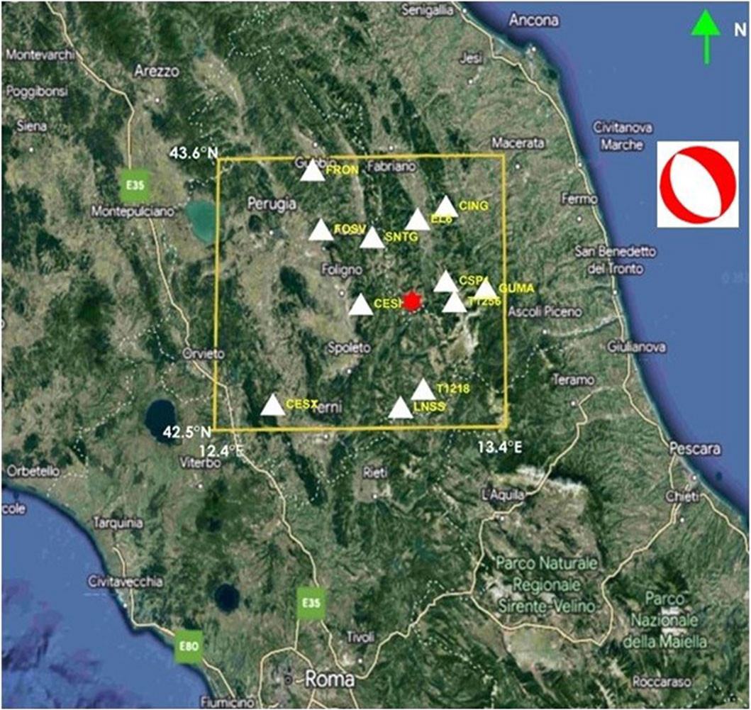
Figure 4. Location of the events and seismic stations considered in this study. The red star indicates the epicenters of MAIN and EGF. The white triangles indicate the seismic stations used in the inversion of source parameters. The station names are reported in yellow characters. The focal mechanism of the MAIN is also shown.
In our data selection process, we focused on seismic stations located within 100 km of the event epicenters (Table 3). Among these stations, we selected twelve three-component recordings characterized by a clear onset of the first P-wave of the EGF and waveform similarities between EGF and MAIN, as required by the assumptions of the EGF technique.
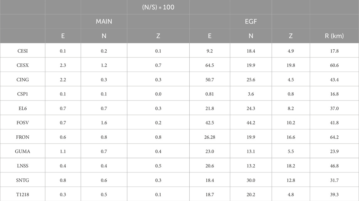
Table 3. Percentage noise-to-signal (N/S) ratio at the three components of MAIN and EGF and source (MAIN)-to receiver distance R. E indicates the East component, W indicates the West component and Z indicates the vertical component of waveforms.
To include the possibility that rupture occur in a supershear regime (Vs.≤Vr) the present method can be applied only to P-waves and their coda. DFB showed in fact that the range of applicability of the Sato (1994) is the subsonic regime (Vs.≤Vr≤Vp) only when using P-waveforms. This is because the apparent moment rate inferred by Sato (1994) holds for any seismic phase whose velocity c satisfies the relation Vr≤c. Therefore, the inclusion of S waves would limit the application of the technique to the subshear regime.
The spectra of EGF exhibit a corner frequency (fc) ranging between 10 and 12 Hz, while the spectra of MAIN have a corner frequency of about 6 Hz. These corner frequencies are highlighted in the normalized average spectrum plots (Houston and Kanamori, 1986), shown in Figure 5. The scaling between the corner frequency and the inverse of pulse width implies that the source pulse width of EGF should be less than about one-half that of the MAIN, aligning with the assumption of the method proposed by DFB.
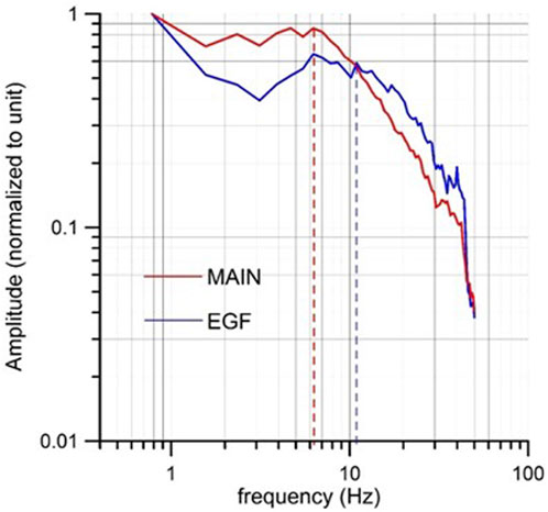
Figure 5. Average common spectrum of the MAIN and the EGF. The vertical shadow lines intercept, on the horizontal axis, the corner frequency of the two events.
To prepare the seismic waveforms for analysis, we applied low-pass filtering below the corner frequency of EGF. The average level of noise (N) was calculated as the average absolute amplitude in a 0.5-s time window preceding the P-wave arrival, while the average level of signal (S) was computed as the average absolute amplitude in a 0.5-s time window following the P-wave arrival. As summarized in Table 3, recordings of MAIN exhibit a very low noise-to-signal ratio (N/S), which is clearly correlated with the source to receiver distance. Conversely, recordings of EGF show varying levels of noise, with N/S ratios ranging from a minimum of 0.8% to a maximum of 64.5%, indicating significant noise interference in some cases.
3.1 Inversion results
In the first inversion step, we considered different time windows (TL) ranging from TL = 0.7 s to TL = 1.3 s. The starting time of TL was set at 0.2 s before the picked P-wave arrival on non-filtered traces to accommodate potential misalignments in the P-wave onset between EGF and MAIN. At the end of our trials, the optimal time window (TL = 0.9 s) was determined as the one that minimized the overall misfit function. It is important to note that, for TL = 0.9 s, the overall window includes both the first P-waveform (having a pulse width of about 0.2 s) and a substantial part of its coda, lasting approximately 0.5 s. In this way not only the first P-pulse is considered, as done in DFB, but also the main part of the radiated P-wave energy. In the inversion, we considered a total number
The model parameter estimates obtained for each station after the first inversion step are summarized in Table 5. These estimates typically exhibit variability among stations. The retrieved source radius can be categorized into two distinct ranges: (0.1 km ≤ L ≤ 0.22 km; Δσ ≥ 2 MPa) and (L ≥ 0.30 km; Δσ ≤ 1 MPa). A smaller source radius is generally associated with a higher stress drop, indicative of the well-known correlation between these parameters.
The comparison between observed and theoretical seismograms (Figure 6) generally shows a very good match and, in some cases, an excellent match, as evidenced by the low values of the misfit function (reported in Table 4), despite the presence of significant noise affecting many EGF recordings. This robust result was also observed in the synthetic test with the noisiest EGF (Figure 3).
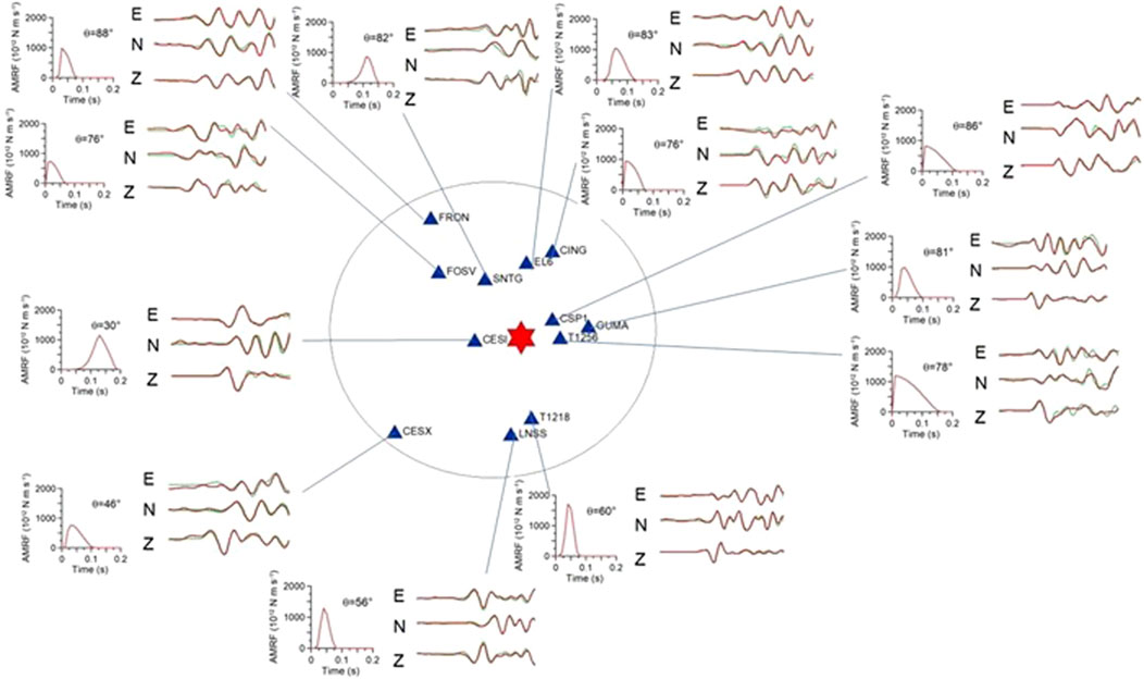
Figure 6. Comparison between observed (green) and theoretical (red) mainshock as a function of the source-to-receiver azimuth, after the first step of inversion. The lines connecting stations and seismograms are oriented approximately along the source-to-receiver azimuth. For each station the retrieved Sato (1994) AMRF is also shown.
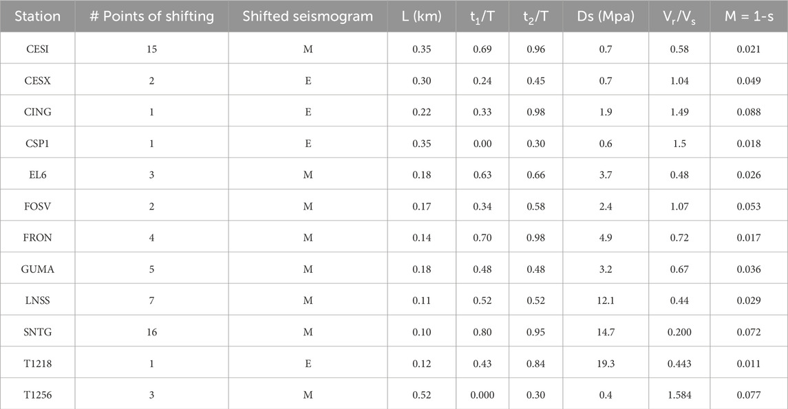
Table 4. Results of the first step of inversion for the studied event.
In the second step of the inversion process, we computed the optimal alignments of MAIN and EGF for each model parameter station solution obtained in the first step (refer to Table 4). This involved determining the combination of alignments that minimized the misfit function across all available stations, while keeping the model parameters fixed at the values obtained in the initial step. Once we identified the optimal alignments for each model parameter station solution, we selected the best combination corresponding to the absolute minimum of the inferred misfit functions (see Figure 7). For the event under study, the optimal combination of alignments was determined using the model parameter solution obtained for station GUMA in the first step.

Figure 7. Plot of the minimum misfit M = 1-s (non-dimensional) vs. the station name at the second step of inversion (see the text). Each point represents the absolute minimum among the misfit values that are obtained by fixing the model parameters at the values obtained at the first step at that station and letting vary the alignments between MAIN and EGF at all the other stations. The absolute minimum among these is found when we consider the model parameters found for station GUMA (sky-blue star) at the first step of inversion.
After fixing the selected alignments, we employed the grid-search method to compute the values of the likelihood function
where:
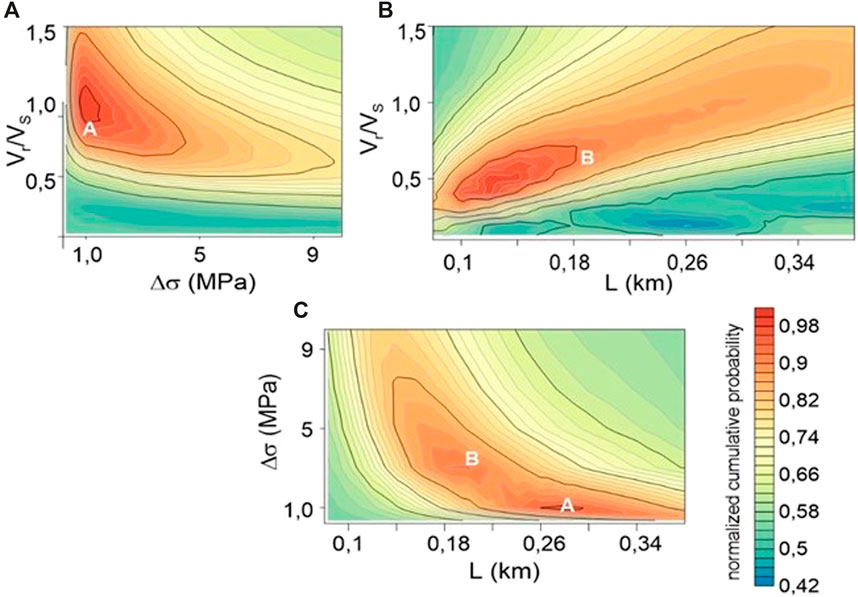
Figure 8. Plot of the normalized cumulative probability density functions (CPDF). In each map A and B indicate the position of the two inferred best fit solutions (A and B, Table 5) in the three planes. (A) CPDF in the plane [Δσ, Vr/Vs]; (B) CPDF in the plane [L,Vr/Vs]; (C) CPDF in the plane [L, Δσ].
Instead, by mapping (Figure 8B) in the [L,Vr/VS] plane the CPDF described by the equation:
a larger correlation area, that includes only the solution B, is found.
Finally, a large correlation area, but enclosing only the solution A, is also found (Figure 8C) when mapping, in the [Δσ,Vr/VS] plane, the CPDF described by the equation:
Figure 9 illustrates the fit of synthetic waveforms to observed waveforms for solution B. A minor reduction in the quality of fitting compared to the single station inversion case (Figure 6) is observed. This reduction is statistically expected because the number of degrees of freedom decreases from ndf = 12 × 5 = 60 for the single station inversion to ndf = 5 for the case of a single rupture model.
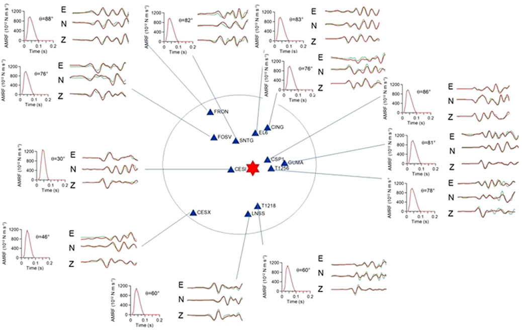
Figure 9. Comparison between observed (green) and theoretical (red) mainshock as a function of the source-to-receiver azimuth, for the preferred solution. The lines connecting stations and seismograms are oriented approximately along the source-to-receiver azimuth. For each station the retrieved Sato (1994) AMRF is also shown.
Model parameters and their associated errors (refer to Table 5) were computed as weighted averages, using the following relationships:
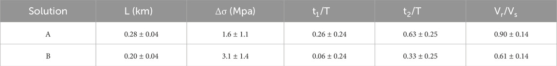
Table 5. The two model parameter solutions for the event considered in this study.
In Eqs 23, 24, V represents the volume of a polyhedron, defined in the five-dimensional parameter space, centered on each maximum of the likelihood function, and excluding secondary maxima. The choice of V was performed by analyzing the shape of the correlation maps of the model parameter couples around the maximum (Figures 10, 11).
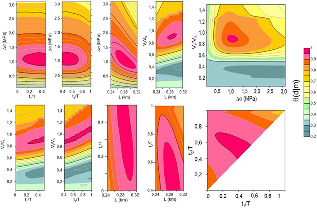
Figure 10. Correlation maps for the solution A. the values of the likelihood function are contoured as a function of each couple of model parameters
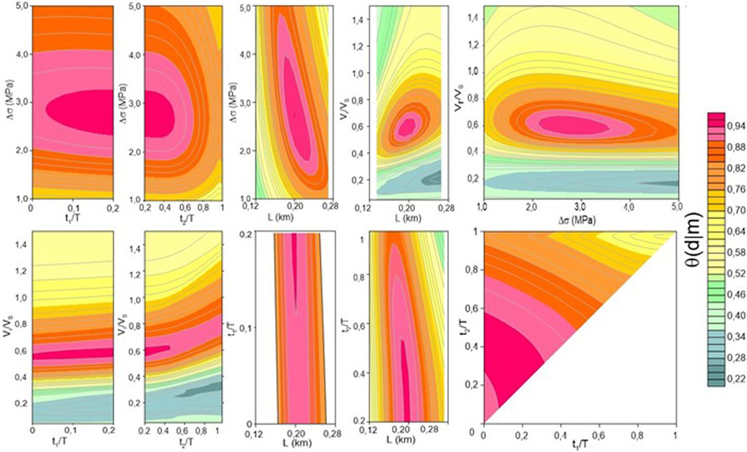
Figure 11. Correlation maps for the solution B. The values of the likelihood function are contoured as a function of each couple of model parameters
3.2 Heterogeneous rupture model vs. circular crack model
To determine whether the inferred circular crack models A and B are better representatives of the source process compared to the heterogeneous fault model inferred in the first step, we utilized the corrected Akaike information criterion (AICc), which summarizes the Occam’s Razor principle. According to the AICc (also used in DFB), when comparing two models describing the data, the preferred model is the one that minimizes the quantity given by Akaike (1973):
In Eq. 25 k is the number of model parameters, npt is the overall number of points of seismograms involved in the inversion and:
Eq. 26 computes the weighted squared residual between data and data predicted by the model. For the heterogeneous model obtained after the first step of inversion and summarized in Table 4, we obtained AICc = 61749. Instead, for the circular crack models A and B summarized in Table 5, we obtained respectively AICc = 56900 and AICc = 56961. Therefore, for the studied event, a circular crack model with variable rupture velocity better represents the source model compared to the heterogeneous fault model that could be derived from the back-projection of the single station solutions.
4 Discussion and conclusion
Upon analyzing the results presented in Table 5 and examining the correlation maps depicted in Figures 10, 11, it is evident that the parameters most affected by uncertainty are the durations of both the nucleation (t1) and deceleration (t2) phases. Despite the significant percentage error associated with estimating these parameters, models A and B, which are considered most likely, demonstrate that rupture velocity varies during the rupture process. Specifically, for model A, the correlation maps in Figure 10 suggest the existence of a nucleation phase (t1/T≠0), while the deceleration phase is less clear. Conversely, the correlation maps in Figure 11 suggest that for model B, a deceleration phase (t2/T<1) is necessary, with the nucleation phase being less resolved. Thus, regardless of the preferred model choice, the rupture process must involve either a nucleation or a deceleration phase. Model B, characterized by a minimal nucleation phase, aligns closely with Boatwright’s (1980) original causal decelerating model. These observations, coupled with the ability of the model to reproduce the initial P-wave pulse across all azimuths (Figure 9), indicate that circular crack models with variable rupture velocity overcome the limitations of simplified circular crack models with constant rupture velocity (Brune, 1970; Sato and Hirasawa, 1973) in accurately modeling P-waveform shapes.
The errors affecting source radius, rupture velocity, and stress drop are notably small, as indicated by the visual examination of the maps in Figures 10, 11, along with the error estimates provided in Table 5. Consequently, the inferred stress drops using this method are more constrained compared to those typically derived from seismic spectra inversion (e.g., de Lorenzo et al., 2010; Abercombie, 2021). This improvement arises because EGF techniques incorporate site effects in the empirical Green’s function, whereas in seismic spectra inversions site effects are usually estimated as average residuals between observed and retrieved spectra.
As discussed in the introduction section, higher is the rupture velocity and higher is the fraction of the accumulated energy radiated by an earthquake. Interestingly, the two most probable Vr/VS (rupture velocity to shear wave velocity) ratios identified in this study (0.61 and 0.9) lie at the edges of the previously reported range of variability (0.65 < Vr/VS < 0.85) from earlier studies (Heaton, 1990), suggesting a potential sub-shear regime for the analyzed event. However, for solution A, the results do not entirely rule out a super-shear regime. Specifically, the correlation map in the [Vr/Vs, t2/T] plane indicates that the maximum likelihood region [θ (d|m) ∼ 0.95] corresponds to cases where Vr/VS > 1, coupled with a shorter duration of the deceleration phase. Exploring rupture velocity in Central Italy could be critical for enhancing seismic hazard assessment in the region. Notably, recent research has highlighted the significant role of pore fluid-pressure effects in increasing rupture velocity (Pampillon et al., 2023). This phenomenon might also apply to Central Italy, where the local tectonic regime is influenced by fluid-filled crack systems parallel to thrust fronts (see de Lorenzo and Trabace, 2011, and references therein).
Whereas significant advances have been made in constraining the rupture velocity of great magnitude earthquakes (see Bouchon and Valle, 2003 and references therein), rupture velocity of a small earthquakes remains one of the parameters less constrained by seismological methods, that are generally based on the assumption of a constant rupture velocity. Therefore, future studies should focus more deeply on this important parameter, using more realistic rupture models than a simple circular crack model rupturing at a constant velocity.
The correlation among the most constrained parameters (Δσ, Vr, and L) is clear from the cumulative probability distribution function (CPDF described by the Eqs 19-22) plots of Figure 8, where the effects of nucleation and deceleration phase are averaged out. When analyzing couple of parameters, the correlation becomes weaker (Figures 10, 11). This observation indicates that the introduction of a nucleation and deceleration phase in the rupture process can significantly reduce the correlation between stress drop, rupture velocity and source radius. The CPDF plots confirm the anticorrelation between Δσ and L found in previous studies (Abercombie, 2021), indicating that an increase in Δσ is typically associated with a decrease in L. This correlation aligns with the constraint provided by the Eshelby (1957) relationship (Eq. 10) applied to quasi-dynamic source models.
A more contentious issue arises regarding the potential anti-correlation between Δσ and Vr (Chounet et al., 2018). The CPDF map in the [Δσ, Vr] plane (Figure 8) suggests that this correlation significantly impacts our findings. Theoretically, this correlation arises from the Eshelby (1957) relationship, particularly when considering the interaction between source rise time, source dimension, and rupture velocity inherent in all quasi-dynamic source models (as expressed in Eqs 18, 19 of Deichmann, 1997). Consequently, our results support the working hypothesis proposed by Causse and Song (2015), which postulates that this anti-correlation reduces the variability in predicted peak-ground acceleration (PGA), aligning it more closely with observed PGA values.
Furthermore, the evident correlation between L and Vr (Figure 8) can be readily explained by recalling that these two parameters are linked by the following equation: that arises from Eq. 6 of Deichmann (1997) for the case of a constant acceleration phase.
Between the two obtained solutions A and B, we opted for solution B as the preferred choice, despite its slightly lower likelihood value (0.95 vs. 0.954). This decision was based on two main reasons. Firstly, upon visually inspecting the waveform fitting, we observed that model B tends to reproduce the first P-pulse across all stations more accurately, whereas model A performs better in reproducing the P-wave coda. Notably, the results were obtained by using a sufficiently wide time window (TL = 0.9 s), which includes several secondary arrivals following the first P-pulse. Secondly, considering scaling laws from seismic events in the same area during a prior 1997 seismic sequence, it was noted that source radii are consistently smaller than 250 m for ML<3.5 (de Lorenzo et al., 2010). This information further supports the preference for solution B in our study.
The differences observed in the retrieved AMRFs after the initial inversion step (as shown in Table 4) suggest a heterogeneous rupture process that deviates from a simple circular crack model with variable rupture velocity. Typically, in such cases, researchers might consider using the estimates from the initial inversion step to infer the slip function on the fault plane through back-projection of station slip functions onto the fault plane, a technique also employed for small magnitude earthquakes (Festa and Zollo, 2006; Stabile et al., 2012). However, for the studied event, we ruled out this possibility by comparing the values of corrected AICc obtained after both inversion steps. This comparison led us to conclude that, in this case, a circular crack model with variable rupture velocity can better reproduce the main properties of P-wave seismic radiation observed at various azimuths and distances compared to a heterogeneous model. This finding is particularly intriguing given that the selected time window (TL = 0.9 s) also includes a significant portion of the P-wave coda. Nevertheless, the non-uniqueness inherent in seismic source inversion (Das, 2015) and the determination of an optimal time window (TL = 0.9 s) for our analysis suggest that other quasi-dynamic crack models (e.g., Dong and Papageorgiou, 2002; 2003) or techniques (e.g., Festa and Zollo, 2006; Cuius et al., 2023) may produce equivalent or superior results with different choices of TL. Moving forward, one key challenge in future seismic source studies should involve comparing results obtained from different techniques and developing a multi-scale approach in the time domain to determine the optimal time extent at which a circular crack model truly represents the optimal source model for small magnitude earthquakes.
A further test has been made by considering only the stations characterized by a high noise-to signal ratio (Cesx, Cing, Fosv, Fron, Sntg, see Table 3) but we obtained, as expected, a reduction of the quality of fitting (the maximum of likelihood function at the second step reduces to 0.87). Therefore, the optimal configuration for this method would consist of using both waveforms having a smaller noise-to signal ratio, which constrain the alignment between MAIN and EGF at the second step, and waveforms having a higher noise-to-signal ratio, which allow to reduce the correlation between model parameters.
One limit of the present model is its non-applicability to the case of unilateral faults. In these cases, it is in-fact expected that observed waveforms will exhibit a clear dependence of the pulse width and/or amplitude variations with the source-to-receiver azimuth, and the present formulation, based on the directivity function of a circular crack, cannot be adopted to retrieve the corresponding source parameters. However, the structure of the inversion method presented in this article will remain valid also in this case, by adopting the appropriate source model for this situation.
The method presented in this article addresses challenges associated with using noisy EGF, as described in DFB, to evaluate whether a circular crack model with variable rupture velocity accurately represents the source process of a small magnitude earthquake. This technique enables the determination of whether such a model is representative of the source process by allowing for a quantitative assessment of the multiplicity of solutions and correlations among model parameters using the Bayesian formulation described. This approach overcomes the local analysis typically achievable with random deviates techniques, providing a more comprehensive and robust framework for seismic source characterization.
The method presented in this paper uses strike and dip fault inferred from fault mechanism solution. In a future study it has to be evaluated if strike and dip fault can be inferred from the joint inversion of P-waveforms and P polarities.
Data availability statement
Publicly available datasets were analyzed in this study. This data is available by request to corresponding author.
Author contributions
SdL: Writing–review and editing, Writing–original draft, Visualization, Validation, Supervision, Software, Resources, Project administration, Methodology, Investigation, Funding acquisition, Formal Analysis, Conceptualization. MM: Writing–review and editing, Visualization, Validation, Supervision, Investigation, Formal Analysis, Data curation.
Funding
The author(s) declare that financial support was received for the research, authorship, and/or publication of this article. This study was financially supported by PRIN-MIUR Italian research funds. It is also part of the European PNRR project “PE RETURN: Multi-risk science for resilient communities under a changing climate—Volcanoes and Earthquakes.”
Acknowledgments
Marilena Filippucci is acknowledged for furnishing the Fortran codes used in the DFB article.
Conflict of interest
The authors declare that the research was conducted in the absence of any commercial or financial relationships that could be construed as a potential conflict of interest.
Publisher’s note
All claims expressed in this article are solely those of the authors and do not necessarily represent those of their affiliated organizations, or those of the publisher, the editors and the reviewers. Any product that may be evaluated in this article, or claim that may be made by its manufacturer, is not guaranteed or endorsed by the publisher.
References
Abercrombie, R. E. (2021). Resolution and uncertainties in estimates of earthquake stress drop and energy release. Phil. Trans. R. Soc. A. 379 (2196). doi:10.1098/rsta.2020.0131
Akaike, H. (1973). “Information theory as an extension of the maximum likelihood principle,” in Second international symposium on information theory. Editors B. N. Petrov, and F. Csaki (Budapest: Akademiai Kiado), 267–281.
Aki, K., and Richards, P. G. (2002). Quantitative seismology. 2nd Edition. Sausalito, CA: Univ. Sci. Books, 700.
Bernard, P., and Madariaga, R. (1984). A new asymptotic method for the modeling of nearfield accelerograms. Bull. Seismol. Soc. Am. 74, 539–557. doi:10.1785/bssa0740020539
Bertero, M., Bindi, D., Boccacci, P., Cattaneo, M., Eva, C., and Lanza, V. (1997). Application of the projected Landweber method to the estimation of the source time function in seismology. Inverse Probl. 13, 465–486. doi:10.1088/0266-5611/13/2/017
Boatwright, J. (1980). A spectral theory for circular seismic sources: simple estimates of source dimension, dynamic stress drop and radiated seismic energy. Bull. Seismol. Soc. Am. 70, 1–28. doi:10.1785/BSSA0700010001
Bouchon, M., and Vallée, M. (2003). Observation of long supershear rupture during the magnitude 8.1 kunlunshan earthquake. Science 301, 824–826. doi:10.1126/science.1086832
Brune, J. N. (1970). Tectonic stress and the spectra of seismic shear waves from earthquakes. J. Geophys. Res. 75, 4997–5009. doi:10.1029/JB075i026p04997
Causse, M., and Song, S. G. (2015). Are stress drop and rupture velocity of earthquakes independent? Insight from observed ground motion variability. Geophys. Res. Lett. 42, 7383–7389. doi:10.1002/2015GL064793
Chiaraluce, L., Di Stefano, R., Tinti, E., Scognamiglio, L., Michele, M., Casarotti, E., et al. (2017). The 2016 central Italy seismic sequence: a first look at the mainshocks, aftershocks, and source models. Seismol. Res. Lett. 88 (3), 757–771. doi:10.1785/0220160221
Chiaraluce, L., Michele, M., Waldhauser, F., Tan, Y. J., Herrmann, M., Spallarossa, D., et al. (2022). A comprehensive suite of earthquake catalogues for the 2016-2017 Central Italy seismic sequence. Sci. Data 9 (1), 710. doi:10.1038/s41597-022-01827-z
Chounet, A., Vallée, M., Causse, M., and Courboulex, F. (2018). Global catalog of earthquake rupture velocities shows anticorrelation between stress drop and rupture velocity. Tectonophysics 733, 148–158. doi:10.1016/j.tecto.2017.11.005
Cuius, A., Meng, H., Saraò, A., and Costa, G. (2023). Sensitivity of the second seismic moments resolution to determine the fault parameters of moderate earthquakes. Front. Earth Sci. 11, 1198220. doi:10.3389/feart.2023.1198220
Das, S. (2015). “Supershear earthquake ruptures – theory, methods, laboratory experiments and fault superhighways: an update,” in Perspectives on European earthquake engineering and seismology. Vol. 2, geotechnical, geological and earthquake engineering. Editor A. Ansal (Springer), 39, 1–20. doi:10.1007/978-3-319-16964-4
Deichmann, N. (1997). Far-field pulse shapes from circular sources with variable rupture velocities. Bull. Seismol. Soc. Am. 87 (5), 1288–1296. doi:10.1785/BSSA0870051288
de Lorenzo, S., Filippucci, M., and Boschi, E. (2008). An EGF technique to infer the rupture velocity history of a small magnitude earthquake. J. Geophys. Res. 113, B10314. doi:10.1029/2007JB005496
de Lorenzo, S., and Trabace, M. (2011). Seismic anisotropy of the shallow crust in the Umbria–Marche (Italy) region. Phys. Earth Planet. Int. 189, 34–46. doi:10.1016/j.pepi.2011.09.008
de Lorenzo, S., Zollo, A., and Zito, G. (2010). Source, attenuation, and site parameters of the 1997 Umbria-Marche seismic sequence from the inversion of P wave spectra: a comparison between constant QP and frequency-dependent QP models. J. Geophys. Res. 115, B09306. doi:10.1029/2009JB007004
Dong, G., and Papageorgiou, A. S. (2002). Seismic radiation from a unidirectional asymmetrical circular crack model, Part II: variable rupture velocity. Bull. Seismol. Soc. Am. 92 (3), 962–982. doi:10.1785/0120010209
Dong, G., and Papageorgiou, A. S. (2003). On a new class of kinematic models: symmetrical and asymmetrical circular and elliptical cracks. Phys. Earth Planet. Int. 137, 129–151. doi:10.1016/S0031-9201(03)00012-8
Ellsworth, W. L., and Beroza, G. C. (1998). Observation of the seismic nucleation phase in the Ridgecrest, California, earthquake sequence. Geophys. Res. Lett. 25 (2), 401–404. doi:10.1029/97GL53700
Eshelby, J. D. (1957). The determination of the elastic field of an ellipsoidal inclusion, and related problems. Proc. R. Soc. Lond. 241, 376–396. doi:10.1098/rspa.1957.0133
Festa, G., and Zollo, A. (2006). Fault slip and rupture velocity inversion by isochrone backprojection backprojection. Geophys. J. Int. 166 (2), 745–756. doi:10.1111/j.1365-246X.2006.03045.x
Hartzell, S. (1978). Earthquake aftershocks as Green’s functions. Geophys. Res. Lett. 5 (1), 1–4. doi:10.1029/GL005I001P00001
Heaton, T. H. (1990). Evidence for and implications of self-healing pulses of slip in earthquake rupture. Phys. Earth Planet. Inter. 64, 1–20. doi:10.1016/0031-9201(90)90002-F
Houston, H., and Kanamori, H. (1986). Source spectra of great earthquakes: teleseismic constraints on rupture process and strong motion. Bull. Seismol. Soc. Am. 76 (1), 19–42. doi:10.1785/BSSA0760010019
Hu, C., Stoffa, P., and McIntosh, K. (2008). First arrival stochastic tomography: automatic background velocity estimation using beam semblances and VFSA. Geoph. Res. Lett. 35 (23), L23307. doi:10.1029/2008GL034776
Latorre, D., Di Stefano, R., Castello, B., Michele, M., and Chiaraluce, L. (2023). An updated view of the Italian seismicity from probabilistic location in 3D velocity models: the 1981–2018 Italian catalog of absolute earthquake locations (CLASS). Tectonophysics 846, 229664. doi:10.1016/j.tecto.2022.229664
Madariaga, R. (1976). Dynamics of an expanding circular fault. Bull. Seismol. Soc. Am. 66, 639–666. doi:10.1785/BSSA0660030639
Madariaga, R. (1977). High-frequency radiation from crack (stress drop) models of earthquake faulting. Geophys. J. Int. 51, 625–651. doi:10.1111/j.1365-246X.1977.tb04211.x
Madariaga, R. (2007). Seismic source theory. Treatise Geophys., 59–82. doi:10.1016/b978-044452748-6.00061-4
Madariaga, R., and Ruiz, S. (2016). Earthquake dynamics on circular faults: a review 1970–2015. J. Seismol. 20, 1235–1252. doi:10.1007/s10950-016-9590-8
Malagnini, L., and Munafò, I. (2018). On the relationship between ML and Mw in a broad range: an example from the Apennines, Italy. Bull. Seismol. Soc. Am. 108 (2), 1018–1024. doi:10.1785/0120170303
Michele, M., Chiaraluce, L., Di Stefano, R., and Waldhauser, F. (2020). Fine-scale structure of the 2016–2017 Central Italy seismic sequence from data recorded at the Italian National Network. J. Geophys. Res. Solid Earth 125 (4), e2019JB018440. doi:10.1029/2019jb018440
Michele, M., Di Stefano, R., Chiaraluce, L., Cattaneo, M., De Gori, P., Monachesi, G., et al. (2016). The Amatrice 2016 seismic sequence: a preliminary look at the mainshock. Ann. Geophys. 59 (Fast Track 5)–2016. doi:10.4401/ag-7227
Mueller, C. S. (1985). Source pulse enhancement by deconvolution of an empirical Green's function. Geophys. Res. Lett. 12 (1), 33–36. doi:10.1029/GL012i001p00033
Pampillón, P., Santillán, D., Mosquera, J. C., and Cueto-Felgueroso, L. (2023). The role of pore fluids in supershear earthquake ruptures. Sci. Rep. 13, 398. doi:10.1038/s41598-022-27159-x
Press, W. H., Flannery, B. P., Teukolsky, S. A., and Vetterling, W. T. (1989). Numerical Recipes, The Art of Scientific Computing (Fortran Version). Cambridge, U. K.: Cambridge Univ. Press.
Sato, T. (1994). Seismic radiation from circular cracks growing at variable rupture velocity. Bull. Seismol. Soc. Am. 84 (4), 1199–1215. doi:10.1785/BSSA0840041199
Sato, T., and Hirasawa, T. (1973). Body wave spectra from propagating shear cracks. J. Phys. Earth 21, 415–431. doi:10.4294/JPE1952.21.415
Shibazaki, B., Yoshida, Y., Nakamura, M., Nakamura, M., and Katao, K. (2002). Rupture nucleations in the 1995 Hyogo-ken Nanbu earthquake and its large aftershocks. Geophys. J. Int. 149 (3), 572–588. doi:10.1046/j.1365-246X.2002.01601.x
Stabile, T. A., Satriano, C., Orefice, A., Festa, G., and Zollo, A. (2012). Anatomy of a microearthquake sequence on an active normal fault. Sci. Rep. 2, 410. doi:10.1038/srep00410
Vallée, M. (2004). Stabilizing the empirical green function analysis: development of the projected landweber method. Bull. Seismol. Soc. Am. 94 (2), 394–409. doi:10.1785/0120030017
Waldhauser, F., and Ellsworth, W. L. (2000). A double-difference earthquake location algorithm: method and application to the northern hayward fault, California. Bull. Seism. Soc. Am. 90, 1353–1368. doi:10.1785/0120000006
Wang, D., Mori, J., and Koketsu, K. (2016). Fast rupture propagation for large strike-slip earthquakes. Earth Planet. Sci. Lett. 440, 115–126. doi:10.1016/j.epsl.2016.02.022
Zollo, A., Capuano, P., and Sing, S. K. (1995). Use of small earthquake records to determine the source time functions of larger earthquakes: an alternative method and an application. Bull. Seismol. Soc. Am. 85 (4), 1249–1256. doi:10.1785/BSSA0850041249
Keywords: circular crack, variable rupture velocity, empirical Green’s function, nucleation and deceleration phase, Bayesian statistics
Citation: de Lorenzo S and Michele M (2024) An EGF technique to infer the source parameters of a circular crack growing at a variable rupture velocity. Front. Earth Sci. 12:1428167. doi: 10.3389/feart.2024.1428167
Received: 05 May 2024; Accepted: 17 June 2024;
Published: 16 July 2024.
Edited by:
Caibo Hu, University of Chinese Academy of Sciences, ChinaReviewed by:
Yong Zhang, Peking University, ChinaYujun Sun, Chinese Academy of Geological Sciences, China
Copyright © 2024 de Lorenzo and Michele. This is an open-access article distributed under the terms of the Creative Commons Attribution License (CC BY). The use, distribution or reproduction in other forums is permitted, provided the original author(s) and the copyright owner(s) are credited and that the original publication in this journal is cited, in accordance with accepted academic practice. No use, distribution or reproduction is permitted which does not comply with these terms.
*Correspondence: Salvatore de Lorenzo, c2FsdmF0b3JlLmRlbG9yZW56b0B1bmliYS5pdA==
†ORCID: Salvatore de Lorenzo, orcid.org/0000-0003-2504-1485