Identification of dominant tree species based on Resource-1 02D hyperspectral image data

Fine-grained classification of tree species by using high-spectral image data has garnered considerable attention from scholars. In this study, through field measurements from Maguan County, Wenshan Prefecture, Yunnan Province, China, high-spectral image data from the Chinese Resource-1 02D satellite were used as the data source. Various analyses were conducted on the original image’s spectral curve, the spectral curve after envelope removal, the spectral curve after first-order differential transformation, and the spectral curve after second-order differential transformation. A spectral angle mapping classification method was employed to classify and identify four dominant tree species in Maguan County, and the accuracy of the classification results was validated using a confusion matrix. Results indicate that the highest accuracy in tree species classification was achieved when first-order differential transformation and envelope removal were used for the spectral curve; the overall accuracy exceeded 95%, and the kappa value was approximately 0.95. The classification results for the spectral curve after second-order differential transformation were the lowest, with an overall accuracy of 81.69% and a kappa value of 0.76. This research demonstrates that applying first-order differential transformation or envelope removal in combination with spectral angle mapping classification considerably reduces data processing time and improves tree species classification accuracy.

1 Introduction

Forest ecosystems are essential components of the earth’s ecosystems. They provide suitable living spaces for flora and fauna while playing a crucial role in environmental protection (Evans, 1939), climate (Herawati and Santoso, 2011) regulation (Thompson et al., 2009), soil and water conservation (Molchanov, 1963), windbreak and sand fixation (Rong et al., 2022), and ecological improvement (Sayer et al., 2004) In recent years, ecological issues (Sovacool, 2014; Liu et al., 2018), such as greenhouse gas emissions, soil erosion, soil degradation, loss of biodiversity, and decreasing water resources, have become increasingly prominent because of forest degradation. Therefore, conducting forest resource inventory to comprehensively and accurately assess the quantity and quality of forest resources has become an indispensable task for governments, forestry departments, and forest management units. This task supports ecological conservation, sustainable forestry development, and modern forest management.

Traditional methods of forest inventory primarily rely on manual surveys, which are characterized by high labor intensity; substantial workload; low efficiency; and high time, labor, and financial costs. Moreover, the complexity of the geographical environment poses risks to survey personnel. As a result, the use of remote sensing technology for forest resource inventory has gradually become a research focus for domestic and international scholars (Leckie, 1990; Boyd and Danson, 2005) Remote sensing images have also become a vital data source in forest resource identification and monitoring (Lei et al., 2016; Pasquarella et al., 2018).

Identifying the types, distribution, and quantity of trees is a crucial aspect of forest resource inventory, and the use of remote sensing imagery for tree species classification has elicited widespread attention from scholars. In early studies, multispectral imagery was an important data source in tree species classification (Zhong et al., 2021). However, its spectral resolution is limited, so accurately differentiating tree species with a similar spectral reflectance is difficult. Typically, only two broad categories, namely, coniferous and broadleaf forests, can be distinguished (Yu, 2013). Hyperspectral imagery presents a new opportunity for fine-grained tree species classification (Zhang et al., 2018), and the use of valuable information within hyperspectral data for precise tree species classification has become a popular research direction (Wang, 2011). Scholars have conducted various studies in this area. For example, Gong et al. used artificial neural networks and successfully classified one broadleaf and six coniferous tree species with an accuracy of up to 90% (Gong et al., 1998). Martin M E et al. combined hyperspectral data to classify 11 tree species on the basis of spectral characteristics and leaf features (Martin et al., 1998). Kumar et al. used 11 sets of leaf spectral reflectance data to differentiate tree species and demonstrated the enhanced distinctiveness of the spectral feature curves after first-order differential transformation (Kumar et al., 2010). In addition, Goodenough et al. classified five forest tree species in Victoria, Canada, by using hyperspectral data and obtained high accuracy of up to 92.9% (Goodenough et al., 2002). Gong Peng et al. used data obtained from a spectrometer to identify six tree species types (Gong et al., 1997). Ding Lixia et al. utilized an envelope removal method and Euclidean distance to identify four tree species and achieved promising results (Ding et al., 2010). Moreover, Wang Lu et al. used HJ-2A hyperspectral imagery to recognize dominant tree species in the Tahe region of Greater Khingan Mountains and achieved the highest accuracy in tree species classification after applying second-order differential transformation to the imagery (Wang and Fan, 2015). Despite these advancements, challenges remain in tree species classification. Machine-based classification methods often require high-quality imagery and are time consuming, leading to reduced classification accuracy. Meanwhile, spectral feature-based methods can be influenced by the spectral signatures of other land cover types, resulting in low classification accuracy and quality. This study combined differential transformation and spectral angle classification methods to enhance the accuracy and general applicability of tree species classification.

This study, which was based on forest inventory field measurements in Maguan County, Wenshan Zhuang and Miao Autonomous Prefecture, Yunnan Province, China, and used high-spectral-resolution remote sensing imagery from the Resource-1 02D satellite, focused on four dominant tree species in Maguan County (Pinus yunnanensis, Alder, Quercus, and China fir). It employed a combination of differential transformation and spectral angle classification methods to develop an efficient, accurate approach for dimensionality reduction and fine-grained classification of tree species by using high-spectral-resolution remote sensing imagery. The study’s findings offer a new, effective method of utilizing spaceborne high-spectral-resolution remote sensing imagery data in forest resource classification and inventory work. This method provides a novel approach and solution and offers reliable data support for forest resource conservation and scientific management.

2 Research area and data

2.1 Study area

Maguan County is located in the southwestern part of Wenshan Zhuang and Miao Autonomous Prefecture, Yunnan Province, China. Its geographical coordinates range from approximately 22°42′to 23°15′north latitude and 103°52′to 104°39′east longitude. It is situated in the southeastern part of Yunnan Province on a low-latitude plateau and is characterized by typical karst topography, as depicted in Figure 1. Maguan County has a diverse and complex terrain, with elevations ranging from a minimum of 123 m to a maximum of 2,579 m above sea level. Consequently, the vertical variation in climate is much more pronounced than the horizontal variation. The region experiences an annual average temperature of 16.9°C, with July being the hottest month (average of 21.7°C) and January being the coldest (average of 9.7°C). The area receives an annual average rainfall of 1,345 mm, enjoys an average of 1,804 h of annual sunlight, and has a frost-free period averaging 327 days, indicating that the area has a subtropical eastern monsoon climate. Maguan County is rich in forestry resources and has high biodiversity, and its forest coverage rate is 56.7%. The county encompasses a total forested area of 163,160 ha, with a total live wood volume of 7.95 million m3. It is primarily home to subtropical evergreen broadleaf forests, mixed coniferous and broadleaf forests, and plantations of tung oil, tea oil, tea, and lacquer trees. This study focused on four dominant tree species in Maguan County, namely, P. yunnanensis, Alder, Quercus, and China fir.

Figure 1

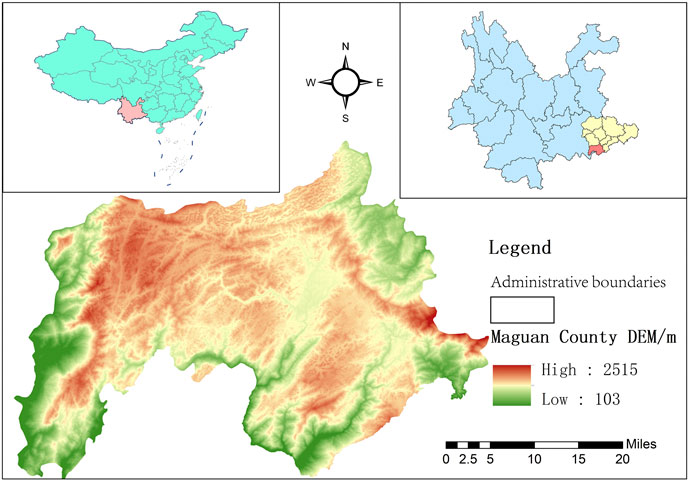
Figure 1. Regional map of the study area.

2.2 Data

The fundamental data used in this study are outlined in Table 1. The data primarily include the following.

(1) Resource-1 02D Hyperspectral Image Data: These data have three images in total, that is, two from 10 November 2020, and one from 6 March 2021, and cover the entire Maguan County region.

(2) Maguan County Administrative Boundary Data: These data provide information on the administrative boundaries of Maguan County.

(3) Digital Elevation Model (DEM) Data: These data offer elevation information on the study area.

(4) Landsat 8 Operational Land Imager (OLI) Data: These data are utilized for various analyses.

(5) Forest Stand Data from Field Surveys: These are obtained from the Maguan County Forestry Bureau and include a total of 8,510 forest stands for the four tree species. Specifically, the data contain 618 P. yunnanensis stands, 1,546 China fir stands, 4,135 Alder stands, and 2,211 Quercus stands.

Table 1

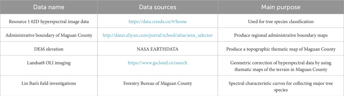
Table 1. Basic data of the study area.

3 Research methods

The overall technical approach used in this study is depicted in Figure 2, and the primary research methods are described in the following subsections.

Figure 2

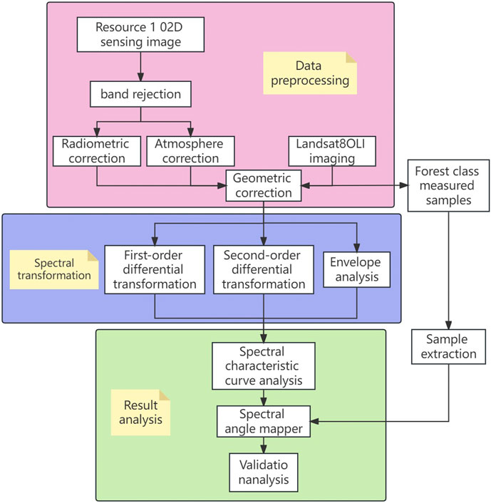
Figure 2. Technical roadmap.

3.1 Data preprocessing

Hyperspectral data are characterized by numerous spectral bands; they contain a wealth of information and often have high data redundancy. Therefore, hyperspectral data need to be preprocessed. The main steps involve the removal of redundant bands, radiometric correction, atmospheric correction, and geometric correction.

The preprocessing procedure in this study began by loading the hyperspectral image via Envi software. Then, the spectral characteristic curves of each band were exported from the image. Subsequently, in Excel, specific bands were removed from the Resource-1 02D hyperspectral image. These excluded bands included fusion bands, water vapor-affected bands, and bands with low signal-to-noise ratios (Table 2). Only the necessary bands for the study were retained, and these included visible and near-infrared (VN) bands 1–71 (395–996 nm), shortwave infrared (SW) bands 1–21 (1,005–1,341 nm), bands 28–47 (1,459–1,778 nm), bands 60–81 (1,997–2,350 nm), and bands 84–87 (2,400–2,450 nm).

Table 2

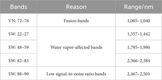
Table 2. Excluded bands of Resource-1 02D satellite.

Next, the Resource-1 02D hyperspectral image was subjected to radiometric calibration and atmospheric correction by using the FLAASH atmospheric correction tool in ENVI software. This process eliminated atmospheric aerosols and other substances that could affect image quality, allowing the image to reflect the true surface reflectance. Figure 3 shows the vegetation spectral reflectance curve before atmospheric correction, and Figure 4 displays the vegetation spectral reflectance curve after atmospheric correction. Afterward, the Resource-1 02D hyperspectral image was geometrically corrected using Landsat 8 OLI imagery as a reference to ensure that the image’s errors were less than 0.5 pixels.

Figure 3

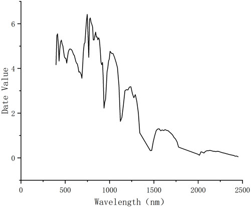
Figure 3. Spectral reflectance curve of vegetation before calibration.

Figure 4

Figure 4. Corrected vegetation spectral reflectance curve.

3.2 Spectral transformation

Applying differential transformation to hyperspectral data can effectively enhance image quality, reduce the influence of the background on vegetation spectral information, improve the signal-to-noise ratio, and further eliminate the effects of atmospheric interference during transformation. Differential transformation allows for a highly accurate representation of the biological composition information of different vegetation types (Shu et al., 2016). This study focused on three transformation methods: first-order differential transformation, second-order differential transformation, and envelope removal.

3.2.1 Spectral first-order differential transformation

Spectral first-order differential transformation involves taking the first derivative of the original remote sensing image data (Gu et al., 2019; Shen, 2022). After this transformation, the image data are less affected by atmospheric radiation, scattering, and atmospheric absorption, enabling the spectral curves to reveal subtle differences between land cover types (Sun et al., 2019). The calculation for spectral first-order differential transformation is given as Eq. 1

${\text{FDR}}_{\lambda \mathrm{t}}=\frac{\text{dR}}{\mathrm{d}\lambda }=\frac{{\mathrm{R}}_{\lambda \mathrm{t}+1}-{\mathrm{R}}_{\lambda \mathrm{t}}}{\Delta \lambda }(1)$

where $\lambda t$ represents the wavelength of the t-th spectral band; FDR_λt is the spectral first-order differential value between the t-th and t+1-th spectral bands; R_λt and R_λt+1 are the original spectral reflectance values for the t-th and t+1-th spectral bands, respectively; and Δλ is generally set to 1.

3.2.2 Spectral second-order differential transformation

Second-order differential transformation involves taking the second derivative of the original remote sensing image data (Yang et al., 2021; Ma et al., 2023). After this transformation, the image data can further amplify differences between different land cover types, thus aiding in identifying sensitive spectral bands (Liu, 2021). The calculation for spectral second-order differential transformation is given as Eq. 2

${\text{SDR}}_{\lambda \mathrm{t}}=\frac{{\mathrm{d}}^2\mathrm{R}}{\mathrm{d}{\lambda }^2}=\frac{\mathrm{d}}{\mathrm{d}\lambda }\left(\frac{\text{dR}}{\mathrm{d}\lambda }\right)=\frac{{\mathrm{R}}_{\lambda t+2}+2R_{\lambda t+1}+R_{\lambda t}}{\left(\Delta {\lambda }^2\right)}(2)$

where $\lambda t$ represents the wavelength of the t-th spectral band; FDR_λt is the spectral second-order differential value between the t-th and t+2-th spectral bands; R_λt and R_λt+1 and R_λt+2 are the original spectral reflectance values for the t-th, t+1-th, and t+2-th spectral bands, respectively; and $\Delta \lambda$ is generally set to 1.

3.2.3 Envelope line division method

The envelope removal method, also known as the continuum subtraction method (Kokaly and Clark, 1999; Ren et al., 2020), is effective in enhancing the absorption, reflection, and emission characteristics of spectral curves. It normalizes the spectral curves to a consistent spectral background, facilitating the comparison of characteristic values between different spectral curves. The reflectance values after envelope removal are normalized to a range between 0 and 1 (Roush and Clark, 1984), with the peak point being one and the other points being less than 1. The final result is the continuum-removed data (Meng et al., 2020). The calculation for envelope removal is presented as Eq. 3

$R_{C_k}=\frac{R_k}{R_{c{r}_k}}(3)$

where R_Ck represents the continuum-removed value for the k-th spectral band, R_k is the original spectral reflectance for the k-th spectral band, and R_Crk represents the continuum for the k-th spectral band (Xie et al., 2005).

3.3 Spectral angle mapping method

Spectral angle mapping (SAM) (Xu et al., 2013; Yu et al., 2016) was introduced by Kruse et al., in 1993 (Kruse et al., 1993). The principle behind using this method in land cover classification is to treat the spectral signature of each pixel in an image as a high-dimensional vector. It measures the spectral similarity between two vectors by calculating the angle between them. A small angle indicates high spectral similarity and a high likelihood that the pixels belong to the same land cover class (Petropoulos et al., 2013; Zhang and Li, 2014) Therefore, unknown data can be categorized based on the size of the spectral angle. In this study, for tree species classification, the spectral angle between unknown and known data was computed, and the unknown data were assigned to the class corresponding to the smallest spectral angle. The calculation formula for SAM is Eq. 4

$\cos \alpha ={\displaystyle \sum _{i=1}^n}\left(x_i\cdot y_i\right)/\left(\sqrt{{\displaystyle \sum _{i=1}^n}{x_i}^2}\cdot \sqrt{{\displaystyle \sum _{i=1}^n}{y_i}^2}\right)(4)$

where $n$ is the number of spectral bands, $x_i$ and $y_i$ represent the response values of the two spectral vectors in the i-th band, and α is the spectral angle whose range of variation is [0, π/2]. The values of the pixels in the spectral angle image can also be expressed using cos(α), which has a variation range of [0, 1].

3.4 Accuracy verification

The Confusion Matrix, also known as the Error Matrix, can accurately reflect the classification results and ground truth information, and reflect the final classification accuracy in a Confusion Matrix. Each column of the confusion matrix represents a ground truth classification, and the value in each column is equal to the number of ground truth pixels corresponding to the corresponding category in the classification image. There are two types of pixel count and percentage representation. By calculating the confusion matrix, two indicators, Overall Accuracy and Kappa coefficient, can be obtained, and the research results can be validated by combining them.

The overall classification accuracy is equal to the correctly classified pixels Eq. (5). The number of correctly classified pixels is distributed along the diagonal of the confusion matrix, and the total number of pixels is equal to the total number of pixels of all real reference sources. The overall classification accuracy calculation formula (5) is shown.

$OA=\frac{pixe{l}_{true}}{pixe{l}_{all}}(5)$

In Eq. 5, it represents the overall classification accuracy, is the correct number of pixels for classification, is the total number of pixels.

Kappa coefficient: It is the sum of the total number of real reference pixels N) multiplied by the diagonal of the confusion matrix (XKK), subtracted by the product of the number of real reference pixels in a certain class and the total number of classified pixels in that class, and then divided by the square of the total number of pixels and subtracted by the product of the total number of real reference pixels in a certain class and the total number of classified pixels in that class to sum all categories Eq. (6). The calculation formula is as follows.

$K=\frac{N{\sum }_k^X-{\sum }_k^{X}k{\sum }^{\mathrm{X}}\sum k}{N^2-{\sum }_k^{\mathrm{X}}k{\sum }^X\sum k}(6)$

4 Analysis of spectral characteristic curve transformation results

4.1 Original spectral characteristic curve

The original spectral characteristic curves for the four tree species in the study area (Quercus, Alder, China fir, and P. yunnanensis) obtained after sampling from the preprocessed Resource-1 02D hyperspectral image data are shown in Figure 5.

Figure 5

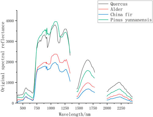
Figure 5. Original spectral characteristic curves of the four vegetation types.

Figure 5 indicates that all four tree species exhibited typical vegetation spectral characteristics, with spectral reflectance increasing then decreasing with the wavelength. Within the wavelength range of 395–996nm, the spectral curves of China fir and Alder overlapped in the range of 775–988 nm. All four tree species showed a reflection peak around 550 nm, with reflectance decreasing between 550 and 679 nm. In this range, distinguishing between China fir and Alder was difficult because their spectral curves overlapped. In the range of 775–988 nm, spectral reflectance of the four tree species was in the order of P. yunnanensis > Quercus > Alder > China fir, indicating distinct differences in reflectance among the four. These differences are favorable for classification. In the range of 1,005–1,173 nm, the spectral reflectance of the four tree species differed considerably, and at 1,072 nm, reflectance reached its maximum value, which was also beneficial for species classification. Within the ranges of 1,459–1,778 and 1,997–2,450 nm, substantial differences in spectral reflectance were observed among the four tree species, which also facilitated tree species classification.

4.2 Spectral characteristic curves after first-order differential transformation

The spectral curve characteristics of vegetation are amplified after first-order differential transformation. The spectral characteristic curves of Quercus, Alder, China fir, and P. yunnanensis are shown in Figure 6.

Figure 6

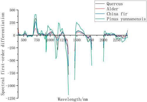
Figure 6. Vegetation curve obtained through first-order differential transformation.

Figure 6 indicates that the spectral characteristic curves of the four tree species exhibited considerable differences. Within the range of 395–413 nm, the curves showed a decreasing trend, but the first-order differential curves of Quercus and P. yunnanensis overlapped and could not be distinguished. In the range of 413–499 nm, the spectral characteristic curves of the four tree species completely overlapped, making them indistinguishable. Within the range of 499–550 nm, the first-order differentials for the four tree species were positive, indicating a positive correlation between their spectral reflectance and wavelength. Additionally, all four tree species exhibited a reflectance peak at 524 nm. Within the range of 559–679 nm, the first-order differential values were negative, and the frequency and amplitude were similar, suggesting a negative correlation between spectral reflectance and wavelength. However, the first-order differential values were ineffective in distinguishing tree species in this range because of their high overlap degree. Within the range of 687–765 nm, the first-order differential values of the four tree species were in the order of P. yunnanensis > Quercus > China fir > Alder. At 730 nm, all four tree species exhibited a maximum first-order differential reflectance peak, and the differences were substantial. Therefore, 730 nm can serve as a feature band for classifying tree species. Another sensitive range was the reflectance peak from 1,475 to 1,644 nm, with the peak located at 1,526 nm. Within this range, the first-order differential values of the four tree species were in the order of P. yunnanensis > Quercus > China fir > Alder, making this range a sensitive band that can be used for differentiation. Moreover, a sensitive band region was found in the range of 1,660–1,750 nm, where a negative peak appeared. The spectral first-order differential values of the four tree species in this range were in the order of Alder > China fir > Quercus > P. yunnanensis. A negative peak was observed at 1,711nm, which can be used as a distinguishing feature band.

4.3 Spectral characteristic curves after second-order differential transformation

The spectral characteristic curves of Quercus, Alder, China fir, and P. yunnanensis after second-order differential transformation are shown in Figure 7.

Figure 7

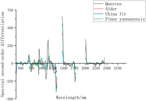
Figure 7. Vegetation curve obtained through second-order differential transformation.

Figure 7 reveals considerable differences in the regions between 524–567 and 622–722 nm. In the range of 524–567 nm, a second-order differential negative peak centered at 550 nm was found, with the second-order differential spectral values ranking in the order of China fir > Alder > P. yunnanensis > Quercus. In the range of 622–722 nm, a second-order differential reflectance peak centered at 696 nm was observed, with the second-order differential spectral values ranking in the order of Quercus > P. yunnanensis > Alder > China fir. The two ranges were effective in distinguishing the four tree species. In the ranges of 928–954 and 1,105–1,173 nm, substantial fluctuation was observed in the second-order differential values of the four bands, which can serve as feature bands for distinguishing the four tree species. Within the 928–954 nm range, the second-order differential value of Quercus was considerably different from the values of the three other species. Alder, China fir, and P. yunnanensis had similar second-order differential values. In the 1,105–1,173 nm range, the reflectance of Quercus peaked at 1,139 nm, and the reflectance of Alder, China fir, and P. yunnanensis peaked at 1,156 nm.

4.4 Spectral characteristic curve after envelope removal

The spectral characteristic curves of Quercus, Alder, China fir, and P. yunnanensis after envelope removal are shown in Figure 8.

Figure 8

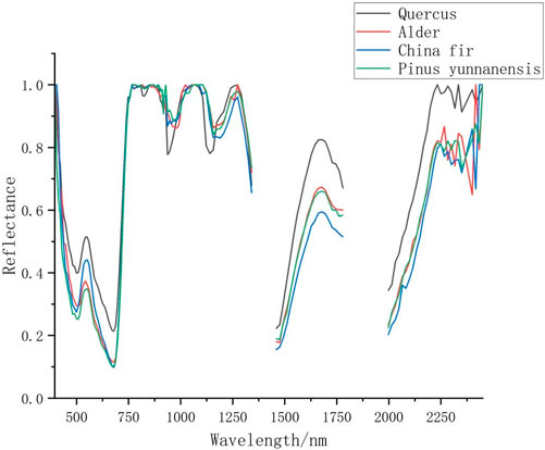
Figure 8. Vegetation curve after envelope removal.

Figure 8 shows considerable differences in the spectral characteristic curves of the four tree species. At 500 nm, a pronounced absorption valley was found, and reflectance was in the order of Quercus > Alder > China fir > P. yunnanensis. At 550 nm, a clear absorption peak was observed, and reflectance was in the order of Quercus > China fir > Alder > P. yunnanensis. At 1,660 nm, a distinct absorption peak was found, and reflectance was in the order of Quercus > Alder > P. yunnanensis > China fir. The three wavelengths were effective for distinguishing the four tree species.

In conclusion, after analyzing the curve feature differences in the preprocessed original spectrum, first-order differential spectrum, second-order differential spectrum, and the spectrum after envelope removal, wavelengths were selected in units of 20 nm from the four types of spectral curves, resulting in 14, 10, 5, and 4 wavelengths, as shown in Table 3. The selected wavelengths were then used for tree species classification.

Table 3

Table 3. Spectral bands with significant differences.

5 Classification results and accuracy evaluation

5.1 Classification results

The pixel spectral curves of the four tree species were analyzed through a field investigation of 226 forest stands. The average spectral curves were used as the spectral reference curves for each tree species. The spectral angle mapping method was employed to classify tree species in the Resource Satellite 02D imagery. The classification results are shown in Figures 9–12. Figure 9 presents the classification results of the preprocessed original image, Figure 11 displays the classification results after envelope removal, Figure 11 shows the classification results after first-order differential transformation, and Figure 12 illustrates the classification results after second-order differential transformation.

Figure 9

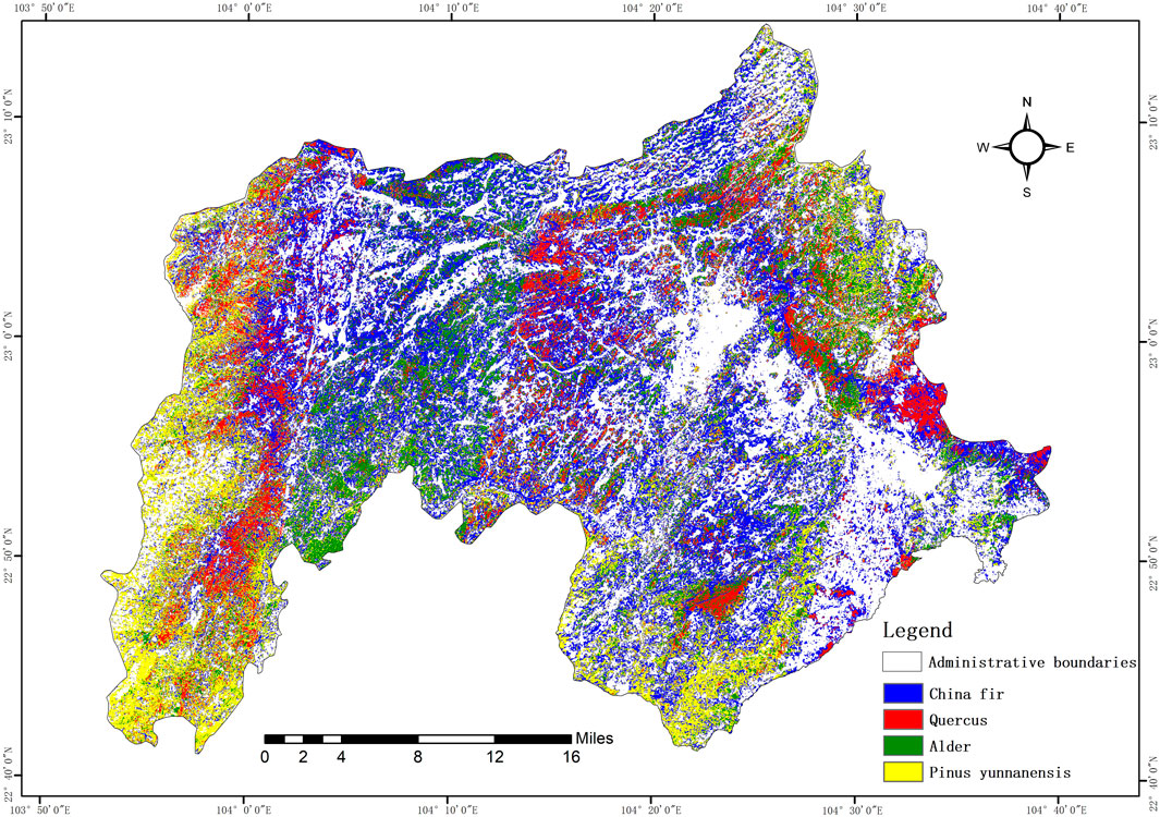
Figure 9. Original image classification results.

Figure 10

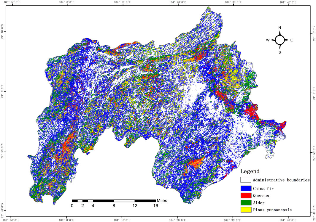
Figure 10. Classification results of de-enveloping lines.

Figure 11

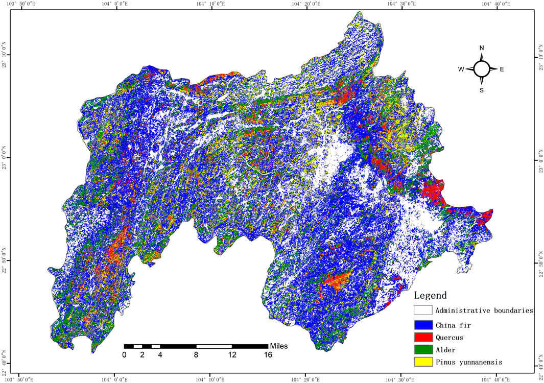
Figure 11. First-order differential transformation classification results.

Figure 12

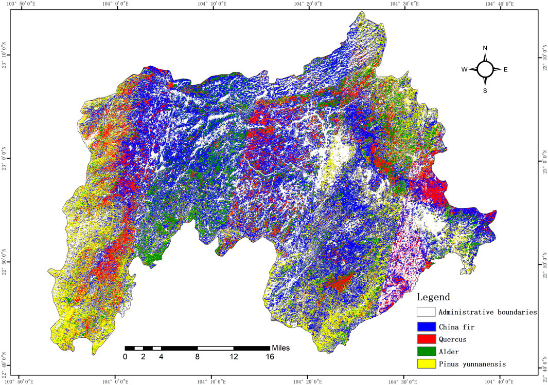
Figure 12. Classification results of second-order differential transformation.

The analysis and comparison of the results revealed that the classification results for the images processed with envelope removal and first-order differential transformation were highly accurate. The classification results for the preprocessed original image and the images processed with second-order differential transformation had low accuracy. The areas with misclassification were mainly the planting areas of P. yunnanensis and China fir. Some China fir areas were misclassified as P. yunnanensis areas, and a small portion of China fir was misclassified as Quercus.

5.2 Precision evaluation

In this study, the accuracy of the classification results was validated using a confusion matrix method (Gonzalez-Alonso et al., 1997). Based on the distribution of tree species in the study area, a total of 226 sampling points were set up, including 68 samples of China fir, 51 samples of Oak, 68 samples of Alder, and 39 samples of Pinus yunnanensis. A total of 288 pixels were obtained from the validation sample points, including 69 for Pinus yunnanensis, 80 for Alder, 75 for Oak, and 64 for China fir. Overall accuracy and the kappa coefficient were used to assess accuracy. Seventy-five percent of the sample pixels were used for classification, and the remaining 25% was used for accuracy validation. The results, which are shown in Table 4, indicate that the classification result from the image processed with second-order differential transformation had the lowest overall accuracy (81.69%) among all the classification results primarily because of the misclassification among P. yunnanensis, China fir, and Quercus. The classification result from the original image (overall accuracy of 88.71%) was slightly higher than that from second-order differential transformation. The accuracy of the classification results for the images processed with envelope removal and first-order differential transformation exceeded 95%, and these results closely matched the field survey data.

Table 4

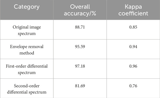
Table 4. Overall accuracy and kappa coefficient statistics.

6 Conclusion and discussion

6.1 Conclusion

This study adopted forestry field survey data for Maguan County in Yunnan and Resource Sat-2 hyperspectral satellite imagery. It also employed three methods, namely, first-order differentiation, second-order differentiation, and envelope removal, to analyze the spectral characteristics of four dominant tree species in Maguan County. The SAM technique was applied for tree species classification, and accuracy validation was conducted. According to the experimental results, the imagery data processed with first-order differentiation and envelope removal effectively enhanced the differentiation between bands and improved the accuracy of species classification. The original imagery and the imagery processed with second-order differentiation had low classification accuracy and showed instances of misclassification. The threshold setting of the matching angle might have affected the spectral classification or complexities in the land cover distribution within mixed pixels and made it challenging to describe real-world objects accurately, resulting in the aforementioned misclassification. Moreover, during the data preprocessing phase, the imagery subjected to atmospheric correction showed that although the spectral characteristics of the vegetation were corrected, the reflectance values were low, which can lead to “same material, different spectrum” or “same spectrum, different material” issues (Zhang et al., 2006; Huang et al., 2022). These factors can also affect classification accuracy.

In summary, using hyperspectral remote sensing data in tree species classification is highly feasible. Methods, such as first-order differentiation and envelope removal, effectively enhance the spectral characteristics of vegetation. Additionally, the use of SAM for classification considerably improves the accuracy of tree species classification.

6.2 Discussion

Currently, hyperspectral data are a reliable data source for tree species classification and can be applied to fine-scale tree species classification in the field of remote sensing. However, previous studies encountered challenges in balancing data processing speed, quality, and accuracy. This research combined three methods, namely, first-order differentiation, second-order differentiation, and envelope removal, with SAM to achieve satisfactory classification results for the study area. However, the study still has some limitations. For instance, the selection of certain tree species areas as the basis for generating average spectral feature curves may lead to inaccuracies if other land cover types exist within the selected regions. Future research should choose pure pixel samples as much as possible and collect ground-truth spectral data through field surveys to further validate the spectral feature curves, thus reducing the influence of other land cover types on the final results. Furthermore, this study focused on Maguan County. Future research could apply the geographic third law to classify and validate tree species with similar geographical environments (Zhu et al., 2018).

Data availability statement

The original contributions presented in the study are included in the article/supplementary material, further inquiries can be directed to the corresponding author.

Author contributions

JZ: Writing–review and editing, Writing–original draft, Visualization, Validation, Supervision, Resources, Methodology, Investigation, Funding acquisition, Formal Analysis, Conceptualization. ZF: Writing–review and editing, Writing–original draft, Visualization, Validation, Project administration, Methodology, Formal Analysis, Data curation, Conceptualization. YL: Writing–review and editing, Visualization, Project administration, Methodology, Investigation, Conceptualization. WJ: Writing–review and editing, Visualization, Validation, Funding acquisition, Supervision, Methodology. XM: Writing–review and editing, Validation, Supervision, Methodology, Formal Analysis. YL: Writing–review and editing, Visualization, Validation, Supervision, Software. SQ: Writing–review and editing, Visualization, Validation, Supervision, Methodology.

Funding

The author(s) declare that financial support was received for the research, authorship, and/or publication of this article. This research was funded by the Funding for Yunnan Province Graduate Supervisor Team Construction Project. Science and Technology Major Project of Yunnan Province (Science and Technology Special Project of Southwest United Graduate School–Major Projects of Basic Research and Applied Basic Research): Vegetation change monitoring and ecological restoration models in Jinsha River Basin mining area in Yunnan based on multi-modal remote sensing (Grant No. : 202302AO370003). The Multi-government International Science and Technologylnnovation Cooperation Key Project of the National Key Research and Development Program olChina for the “Environmental monitoring and assessment of land use/land cover change impact onecological security using geospatial technologies”(2018YFE0184300).

Acknowledgments

We appreciate the forestry data provided by the Forestry Bureau of Maguan County; Free 30 m resolution DEM data and Landsat provided by Geospatial Data Cloud8OLI data; The land observation satellite data service platform provides hyperspectral remote sensing image data.

Conflict of interest

The authors declare that the research was conducted in the absence of any commercial or financial relationships that could be construed as a potential conflict of interest.

Publisher’s note

All claims expressed in this article are solely those of the authors and do not necessarily represent those of their affiliated organizations, or those of the publisher, the editors and the reviewers. Any product that may be evaluated in this article, or claim that may be made by its manufacturer, is not guaranteed or endorsed by the publisher.

References

Boyd, D. S., and Danson, F. (2005). Satellite remote sensing of forest resources: three decades of research development. Prog. Phys. Geogr. 29 (1), 1–26. doi:10.1191/0309133305pp432ra

CrossRef Full Text | Google Scholar

Ding, L., Wang, Z., and Ge, H. (2010). Continuum removal based hyperspectral characteristic analysis of leaves of different tree species. J. Zhejiang A F Univ. 27 (06), 809–814. doi:10.11833/j.issn.2095-0756.2010.06.001

CrossRef Full Text | Google Scholar

Evans, G. (1939). Ecological studies on the rain forest of southern Nigeria: II. The Atmospheric Environmental Conditions. J. Ecol. 27, 436–482. doi:10.2307/2256374

CrossRef Full Text | Google Scholar

Gong, P., Pu, R., and Yu, B. (1997). Conifer species recognition: an exploratory analysis of in situ hyperspectral data. Remote Sens. Environ. 62 (2), 189–200. doi:10.1016/s0034-4257(97)00094-1

CrossRef Full Text | Google Scholar

Gong, P., Pu, R., and Yu, B. (1998). Conifer species recognition with seasonal hyperspectral data. Natl. Remote Sens. Bull. (03), 211–217.

Google Scholar

Gonzalez-Alonso, F., Cuevas, J. M., and Arbiol, R. (1997). Remote sensing and agricultural statistics: crop area estimation in north-eastern Spain through diachronic Landsat TM and ground sample data. Int. J. Remote Sens.18 (2), 467–470. doi:10.1080/014311697219213

CrossRef Full Text | Google Scholar

Goodenough, D. G., Bhogal, A., Dyk, A., Hollinger, A., Mah, Z., Niemann, K. O., et al. (2002). “Monitoring forests with hyperion and ALI,” in IEEE International Geoscience and Remote Sensing Symposium, Toronto, ON, Canada, November 07, 2002 (IEEE).

Google Scholar

Gu, X., Wang, Y., Sun, Q., Yang, G., and Zhang, C. (2019). Hyperspectral inversion of soil organic matter content in cultivated land based on wavelet transform. Comput. Electron. Agric. 167, 105053. doi:10.1016/j.compag.2019.105053

CrossRef Full Text | Google Scholar

Herawati, H., and Santoso, H. (2011). Tropical forest susceptibility to and risk of fire under changing climate: a review of fire nature, policy and institutions in Indonesia. For. Policy Econ. 13 (4), 227–233. doi:10.1016/j.forpol.2011.02.006

CrossRef Full Text | Google Scholar

Huang, P., Pu, J., Zhao, Q., Li, Z., Song, H., and Zhao, X. (2022). Research progress and development trend of remote sensing information extraction methods of vegetation. Remote Sens. Nat. Resour. 34 (2), 10–19. doi:10.6046/zrzyyg.2021137

CrossRef Full Text | Google Scholar

Kokaly, R. F., and Clark, R. N. (1999). Spectroscopic determination of leaf biochemistry using band-depth analysis of absorption features and stepwise multiple linear regression. Remote Sens. Environ. 67 (3), 267–287. doi:10.1016/S0034-4257(98)00084-4

CrossRef Full Text | Google Scholar

Kruse, F. A., Lefkoff, A., Boardman, J., Heidebrecht, K., Shapiro, A., Barloon, P., et al. (1993). The spectral image processing system (SIPS)—interactive visualization and analysis of imaging spectrometer data. Remote Sens. Environ. 44 (2-3), 145–163. doi:10.1016/0034-4257(93)90013-n

CrossRef Full Text | Google Scholar

Kumar, L., Skidmore, A. K., and Mutanga, O. (2010). Leaf level experiments to discriminate between eucalyptus species using high spectral resolution reflectance data: use of derivatives, ratios and vegetation indices. Geocarto Int. 25 (4), 327–344. doi:10.1080/10106040903505996

CrossRef Full Text | Google Scholar

Leckie, D. G. (1990). Advances in remote sensing technologies for forest surveys and management. Can. J. For. Res. 20 (4), 464–483. doi:10.1139/x90-063

CrossRef Full Text | Google Scholar

Lei, G., Li, A., Tan, J., Zhang, Z., Bian, J., Jin, H., et al. (2016). Forest types mapping in mountainous area using multi-source and multi-temporal satellite lmages and decision tree models. Remote Sens. Technol. Appl. 31 (01), 31–41. doi:10.11873/i.issn.1004-0323.2016.1.0031

CrossRef Full Text | Google Scholar

Liu, J., Gao, G., Wang, S., Jiao, L., Wu, X., and Fu, B. (2018). The effects of vegetation on runoff and soil loss: multidimensional structure analysis and scale characteristics. J. Geogr. Sci. 28, 59–78. doi:10.1007/s11442-018-1459-z

CrossRef Full Text | Google Scholar

Liu, Y. (2021). Study on hyperspectral identification Model of typical treeSpecies in changting county. doi:10.27019/d.cnki.gfjsu.2021.000320

CrossRef Full Text | Google Scholar

Ma, C., Liu, X., Li, S., Li, C., and Zhang, R. (2023). Accuracy evaluation of hyperspectral inversion of environmental parameters of loess profile. Environ. Earth Sci. 82 (10), 251. doi:10.1007/s12665-023-10873-8

CrossRef Full Text | Google Scholar

Martin, M., Newman, S. D., Aber, J. D., and Congalton, R. G. (1998). Determining forest species composition using high spectral resolution remote sensing data. Remote Sens. Environ. 65 (3), 249–254. doi:10.1016/S0034-4257(98)00035-2

CrossRef Full Text | Google Scholar

Meng, X., Bao, Y., Liu, H., Zhang, A., Liu, Y., and Wang, D. (2020). Soil classification of typical black soil areas in Northeast China based on high-resolution image No.5. Trans. Chin. Soc. Agric. Eng. 36 (16). doi:10.11975/j.issn.1002-6819.2020.16.028

CrossRef Full Text | Google Scholar

Molchanov, A. A. (1963). The hydrological role of forests.

Google Scholar

Pasquarella, V. J., Holden, C. E., and Woodcock, C. E. (2018). Improved mapping of forest type using spectral-temporal Landsat features. Remote Sens. Environ. 210, 193–207. doi:10.1016/j.rse.2018.02.064

CrossRef Full Text | Google Scholar

Petropoulos, G. P., Vadrevu, K. P., and Kalaitzidis, C. (2013). Spectral angle mapper and object-based classification combined with hyperspectral remote sensing imagery for obtaining land use/cover mapping in a Mediterranean region. Geocarto Int. 28 (2), 114–129. doi:10.1080/10106049.2012.668950

CrossRef Full Text | Google Scholar

Ren, Z., Sun, L., and Zhai, Q. (2020). Improved k-means and spectral matching for hyperspectral mineral mapping. Int. J. Appl. Earth Observation Geoinformation 91, 102154. doi:10.1016/j.jag.2020.102154

CrossRef Full Text | Google Scholar

Rong, Y., Yan, Y., Zhao, C., Wang, C., Shang, X., Zhu, J., et al. (2022). Straw checkboard or afforestation? Assessment and comparison of combined benefits of two typical sand fixing models. J. Clean. Prod. 358, 131924. doi:10.1016/j.jclepro.2022.131924

CrossRef Full Text | Google Scholar

Roush, T., and Clark, R. (1984). Reflectance spectroscopy-quantitative analysis techniques for remote sensing applications. Journal of Geophysical Research. Washington, D.C., United States. American Geophysical Union. 87, 6329–40. doi:10.1029/jb089ib07p06329

CrossRef Full Text | Google Scholar

Sayer, J., Chokkalingam, U., and Poulsen, J. (2004). The restoration of forest biodiversity and ecological values. For. Ecol. Manag. 201 (1), 3–11. doi:10.1016/j.foreco.2004.06.008

CrossRef Full Text | Google Scholar

Shen, C. (2022). Dongchuan red soil Based on GF-5 spectral feature analysisResearch on surface cover identification. Master. Kunming, China: Kunming University of Science and Technology. doi:10.27200/d.cnki.gkmlu.2022.000960

CrossRef Full Text | Google Scholar

Shu, T., Yue, Y., Li, L., Li, R., Li, Y., and Peng, Z. (2016). Crop indentification based on hyperspectral remote sensing. Jiangsu J. Agric. Sci. 32 (06), 1310–1314. doi:10.3969/j.issn.1000-4440.2016.06.018

CrossRef Full Text | Google Scholar

Sovacool, B. K. (2014). Environmental issues, climate changes, and energy security in developing Asia. SSRN Electron. J. doi:10.2139/ssrn.2479725

CrossRef Full Text | Google Scholar

Sun, H., Liu, N., Xing, Z., Zhang, Z., Li, M., and Wu, J. (2019). Parameter Optimization of potato spectral response characteristics and growth stage ldentification. Spectrosc. Spectr. Analysis 39 (06), 1870–1877. doi:10.3964/j.issn.1000-0593(2019)06-1870-08

CrossRef Full Text | Google Scholar

Thompson, I., Mackey, B., McNulty, S., and Mosseler, A. (2009). Forest resilience, biodiversity, and climate change. A synthesis of the biodiversity/resilience/stability relationship in forest ecosystems. Montreal, Canada: Secretariat of the Convention on Biological Diversity

Google Scholar

Wang, L., and Fan, W. (2015). Hyperspectral remote sensing data for ldentifying dominant forest tree species group. J. Northeast For. Univ. 43 (05), 134–137. doi:10.13759/j.cnki.dlxb.20150522.030

CrossRef Full Text | Google Scholar

Wang, Z. (2011). Application Of Hyperspectral Remote Sensing In Forest Tree Species Discrimination. Master. Hangzhou, China: Zhejiang A&F University.

Google Scholar

Xie, B., Xue, X., Liu, W., Wang, J., and Wang, G. (2005). Hull-curve-method-based extraction and analysis of soilspectral characteristics. Acta Pedol. Sin. (01), 171–175. doi:10.3321/j.issn:0564-3929.2005.01.029

CrossRef Full Text | Google Scholar

Xu, Z., Xu, J., Yu, K., Gong, C., Xie, W., Lai, R., et al. (2013). Spectral features analysis of Pinus massoniana with pest of dendrolimus punctatus walker and levels detection. Spectrosc. Spectr. Analysis 33 (02), 428–433. doi:10.3964/j.issn.1000-0593(2013)02-0428-06

PubMed Abstract | CrossRef Full Text | Google Scholar

Yang, C., Feng, M., Song, L., Wang, C., Yang, W., Xie, Y., et al. (2021). Study on hyperspectral estimation model of soil organic carbon content in the wheat field under different water treatments. Sci. Rep. 11 (1), 18582. doi:10.1038/s41598-021-98143-0

PubMed Abstract | CrossRef Full Text | Google Scholar

Yu, L. (2013). The Explore of forest tree species discriminationBased on hyperspectral remote sensing data. Master. Fuzhou, China: Fujian Normal University.

Google Scholar

Yu, L., Yu, y., Liu, X., Du, Y., and Zhang, H. (2016). Tree species classification with hyperspectral lmage. J. Northeast For. Univ. 44 (09), 40–43+57. doi:10.13759/j.cnki.dlxb.2016.09.009

CrossRef Full Text | Google Scholar

Zhang, C., Mu, Y., Yan, T., and Chen, Z. (2018). Overview of hyperspectral remote sensing technology. Spacecr. Recovery and Remote Sens. 39 (3), 104–114. doi:10.3969/j.issn.1009-8518.2018.03.012

CrossRef Full Text | Google Scholar

Zhang, H., Jiang, J., Xie, X., Wu, H., and Zhang, L. (2006). Classification of TM imagery based on the lmproved BP neural network algorithm. J. Agric. Mech. Res. (10), 55–57. doi:10.13427/j.cnki.njyi.2006.10.018

CrossRef Full Text | Google Scholar

Zhang, X., and Li, P. (2014). Lithological mapping from hyperspectral data by improved use of spectral angle mapper. Int. J. Appl. Earth Observation Geoinformation 31, 95–109. doi:10.1016/j.jag.2014.03.007

CrossRef Full Text | Google Scholar

Zhong, H., Liu, H., and Lin, W. (2021). Application of lidar and hyperspectral remote sensing technology to tree species identification. World For. Res. 34 (04), 41–45. doi:10.13348/j.cnki.sjlyyj.2021.0013.y

CrossRef Full Text | Google Scholar

Zhu, A. X., Lu, G., Liu, J., Qin, C. Z., and Zhou, C. (2018). Spatial prediction based on third law of geography. Ann. GIS 24 (4), 225–240. doi:10.1080/19475683.2018.1534890

CrossRef Full Text | Google Scholar