 Lewis J. Gramer
 John Steffen
 Maria Aristizabal Vargas
 Hyun-Sook Kim
94% of researchers rate our articles as excellent or good
Learn more about the work of our research integrity team to safeguard the quality of each article we publish.
Find out more
ORIGINAL RESEARCH article
Front. Earth Sci. , 03 September 2024
Sec. Atmospheric Science
Volume 12 - 2024 | https://doi.org/10.3389/feart.2024.1418016
This article is part of the Research Topic Tropical Cyclone Modeling and Prediction: Advances in Model Development and Its Applications View all 13 articles
Coupling a three-dimensional ocean circulation model to an atmospheric model can significantly improve forecasting of tropical cyclones (TCs). This is particularly true of forecasts for TC intensity (maximum sustained surface wind and minimum central pressure), but also for structure (e.g., surface wind-field sizes). This study seeks to explore the physical mechanisms by which a dynamic ocean influences TC evolution, using an operational TC model. The authors evaluated impacts of ocean-coupling on TC intensity and structure forecasts from NOAA’s Hurricane Analysis and Forecast System v1.0 B (HFSB), which became operational at the NOAA National Weather Service in 2023. The study compared existing HFSB coupled simulations with simulations using an identical model configuration in which the dynamic ocean coupling was replaced by a simple diurnally varying sea surface temperature model. The authors analyzed TCs of interest from the 2020–2022 Atlantic hurricane seasons, selecting forecast cycles with small coupled track-forecast errors for detailed analysis. The results show the link between the dynamic, coupled ocean response to TCs and coincident TC structural changes directly related to changing intensity and surface wind-field size. These results show the importance of coupling in forecasting slower-moving TCs and those with larger surface wind fields. However, there are unexpected instances where coupling impacts the near-TC atmospheric environment (e.g., mid-level moisture intrusion), ultimately affecting intensity forecasts. These results suggest that, even for more rapidly moving and smaller TCs, the influence of the ocean response to the wind field in the near-TC atmospheric environment is important for TC forecasting. The authors also examined cases where coupling degrades forecast performance. Statistical comparisons of coupled versus uncoupled HFSB further show an interesting tendency: high biases in peak surface winds for the uncoupled forecasts contrast with corresponding low biases, contrary to expectations, in coupled forecasts; the coupled forecasts also show a significant negative bias in the radii of 34 kt winds relative to National Hurricane Center best track estimates. By contrast, coupled forecasts show very small bias in minimum central pressure compared with a strong negative bias in uncoupled. Possible explanations for these discrepancies are discussed. The ultimate goal of this work will be to enable better evaluation and forecast improvement of TC models in future work.
Although tropical cyclones (TCs) form from atmospheric circulation features such as baroclinic instability in eastward tropical waves, TC development largely depends on the oceanic conditions beneath. For this reason, a fully coupled dynamic ocean is a necessary component of a TC forecasting model, as it captures the transfer of momentum from the atmosphere to the ocean and the feedback from the ocean to the atmosphere through sea surface temperature (SST) evolution, which modulates air-sea enthalpy fluxes (heat and moisture transfer, hereafter ASEF).
Many early studies highlight the role of the ocean in modulating intensity and ASEF (Riehl, 1950; Sutyrin et al., 1979; Khain and Ginis, 1991; Bender et al., 1993; Schade and Emanuel, 1999). Some early TC modeling studies, e.g., Chang and Anthes (1979) and Chang and Madala (1980), were conducted using constant SST as a lower boundary condition. They concluded that negative feedback with SST is important to TC evolution; those findings led to studies using a one-dimensional ocean model (Wada, 2005; Davis et al., 2008). Limitations in these one-dimensional ocean models, in turn, suggested that dynamic three-dimensional (3D) ocean coupling would provide more accurate feedback and hence better forecasts of the development of TCs, because a coupled 3D ocean provides not only negative but also positive SST feedback depending on the mesoscale structure of the upper ocean and the dynamics of TC-forced ocean circulation (e.g., Bender et al., 1993).
A number of observational studies have demonstrated that upper-ocean thermal structure (Leipper and Volgenau, 1972; Shay et al., 2000; Lin et al., 2009; Jaimes et al., 2015) and the response of the ocean surface boundary layer to TC winds (Cione and Uhlhorn, 2003; Jaimes et al., 2015) play key roles in the intensification of TCs. These studies support the value of full air-sea coupling, in particular with an eddy-resolving ocean model, to simulate multi-scale coevolution of the ocean and TC. Ocean-TC interaction studies have also directly shown the modulation of TC intensity by dynamic ocean response, for example, Wu et al. (2007) and Tuleya and Kurihara (1982).
In addition to intensity, studies have found that coupling impacts other TC features as well. Numerical (Yuan and Jiang, 2011; Yun et al., 2012; Ren et al., 2014; Sun et al., 2017; Yuan and Jiang, 2017) and observational studies (Agrenich, 1984) show the influence of SST on TC track, including left- and right-of-track biases and differences in TC translation speed. Holt et al. (2011) for example, found that TC track error was reduced by ocean coupling at 48 h, although they also found TC track spread increased in coupled vs uncoupled experiments. Similarly, a number of studies have found that coupling can strongly influence forecast storm size (Pun et al., 2021), and specifically storm size can be impacted by SST cooling (Guo et al., 2020; Xu et al., 2020). Previous studies have also highlighted the impact of ocean coupling on large-scale and climate conditions that influence TC activity (Li and Sriver, 2019), e.g., large-scale environmental factors that can modulate TC genesis and seasonal activity. Similarly, previous studies have discussed the importance of both pantropical and TC-TC interaction (Cai et al., 2019; Alaka et al., 2020), which can involve mediation by the ocean. No previous studies, however, have used high resolution modeling to discuss the impact of air-sea coupling on the environment surrounding TCs.
Finally, numerical studies of coupled ocean-atmosphere models have shown that more realistic representations of ocean profiles for temperature and salinity, and of sub-mesoscale currents, are necessary to ensure adequate modeling of ocean response under TC conditions (Halliwell et al., 2011; Jaimes et al., 2011; Le Henaff et al., 2021; Rudzin and Chen, 2023). These previous results highlight the fact, further elucidated in the present work, that the impact of a dynamic ocean on TC forecasts can be different in different ocean regions and oceanographic regimes. Mogensen et al. (2017) for example, showed that in the western Pacific, an uncoupled modeling system produced TCs which were too weak in the southern part of that basin and too intense in the northwest, with important differences in the spatial pattern for their coupled experiment. To date, the present authors are not aware of any similar published results for the Atlantic basin.
The US National Weather Service has a long history of operating coupled ocean-hurricane forecasting systems, including the Geophysical Fluid Dynamics Lab (GFDL) hurricane model since 2002, Hurricane Weather and Forecast System (HWRF) since 2007, and Hurricane Multi-scale Ocean-coupled Non-hydrostatic model (HMON) since 2017. In 2023, the next-generation Hurricane Analysis and Forecast System (HAFS) became an official coupled ocean-hurricane forecast system, intended to replace the legacy HWRF and HMON. The first operational version of HAFS, HAFSv1, has two configurations - HAFS-A (HFSA) and HAFS-B (HFSB). For 2023, both of these systems were coupled with the HYbrid Coordinate Ocean Model (HYCOM) as their ocean component (Bleck et al., 2002).
To simulate two-way air-sea feedback, HYCOM continuously provides updated SST, while it receives net shortwave and longwave radiative fluxes, precipitation rate, sensible and latent heat fluxes, zonal and meridional momentum fluxes, and mean sea level pressure. HYCOM solves 3D primitive ocean equations using scale-dependent lateral mixing and the K-Profile Parameterization (KPP) for vertical mixing (Large et al., 1994). HYCOM has demonstrated forecast skill in coupled hurricane forecast systems running operationally, including HWRF and HMON (Kim et al., 2014; Kim et al., 2022a; Kim et al., 2022b). It accomplishes this skill with evidence-based model parameterizations of physical processes (Kara et al., 2005; Heffner et al., 2008; Rasmussen et al., 2011; L’Hégaret et al., 2015), relying on validation studies for ocean mixing (Kara et al., 2008; Zamudio and Hogan, 2008; Halliwell et al., 2011; Pottapinjara and Joseph, 2022). HYCOM ocean model configurations (Chassignet et al., 2007; Metzger et al., 2014) have been extensively supported by the research community.
The present study investigated changes in TC forecasts with and without HYCOM ocean coupling using HFSB. The goal was to assess the mechanisms by which dynamically evolving SST influences the intensity (maximum sustained surface wind and minimum central pressure), track (center motion), and structure (e.g., surface wind field size, vertical temperature anomaly) of TCs. This work aims to enable future improvements in operational hurricane forecasting capabilities. The paper is organized as follows: Section 1 is this Introduction, Section 2 describes Materials and Methods, Section 3 presents Results, and finally Section 4 is Discussion.
This study evaluated impacts of ocean coupling on TC intensity and structure forecasts from version 1.0 of the HFSB configuration, using an uncoupled version of the model for comparison, as detailed in Section 2.1. Forecast quality metrics were evaluated between the two versions using the Verification tools of the Developmental Test Center Model Evaluation Tools for Tropical Cyclones (MET-TC; Jensen et al., 2023), as well as the GRaphics for OS(s)Es and Other modeling applications on TCs (GROOT) verification package (Ditchek et al., 2023), as described in Section 2.2.
As mentioned above, this study relied on NOAA’s HAFS v1.0B configuration (HFSB), which NOAA made operational in 2023, to provide numerical guidance to operational forecasters in weather centers. HAFS is a tropical cyclone modeling and data assimilation system that is part of NOAA’s Unified Forecast System (UFS) framework. HAFS consists of a regional configuration of NOAA’s FV3 finite-volume atmospheric model (Lin, 2004; Putnam and Lin, 2009) using atmospheric data assimilation, coupled with HYCOM (Bleck et al., 2002) through the Community Mediator for Earth Prediction Systems (CMEPS). More details can be found in Kim et al. (2024, submitted). The HFSB version of HAFS incorporates updated parameterizations for planetary boundary layer (PBL) mass flux and atmospheric microphysics (Hazelton et al., 2023).
HFSB features a regional atmospheric parent domain that is storm-centric and uses an Extended Schmidt Gnomonic (ESG) grid with horizontal resolution of 6 km and an extent of approximately 75 × 75°. It also features a moving nest with a 2 km horizontal resolution and an extent of about 12 × 12°. Its vertical grid has 81 vertical levels with a 2 hPa model top. The HYCOM ocean domain is fixed (non-storm centric) and covers the National Hurricane Center (NHC) areas of responsibility for the North Atlantic, Eastern North Pacific & Central North Pacific basins (23.0°S-47.0°N, 178°W-15.0°E). It has a 1/12-degree horizontal grid spacing and 41 vertical levels.
Atmospheric initial conditions (ICs) and 3-hourly lateral boundary conditions (BCs) for the parent domain are provided by the Global Forecasting System version 16 (GFSv16). In addition, HFSB features vortex initialization (e.g., Lin, 2004), including vortex relocation for all cases, and vortex modification only when the initial storm intensity is at least 30 m/s (58 kt). Four-dimensional ensemble variational (4DEnVar) and First-Guess at Appropriate Time (FGAT) data assimilation techniques are implemented as well. Examples of observations used for assimilation are tail Doppler radar and other airborne reconnaissance observations (Hazelton et al., 2021).
HAFS implements a “warm-start” cycling technique for the atmospheric model, that consists of initializing subsequent forecast cycles from the previous cycle, once the first cycle is completed. For HFSB, the storm intensity at the initial time of a forecast cycle has to be at least 40 kt for warm-start cycling to take place, otherwise the cycle is initialized from GFS initial conditions (“cold start”).
Ocean ICs come from the operational Real Time Ocean Forecasting System (RTOFSv2) with high resolution ocean data assimilation (Garraffo et al., 2020). The ICs consist of temperature, salinity, east and north velocity components, and layer thicknesses from the daily analysis or appropriate RTOFS forecast hour.
Ocean lateral BCs are closed, but the solutions near the domain boundary are relaxed to climatology with an e-folding scale of 30 days within 10 grid cells, while the ICs are integrated at 36 and 10 s using explicit-implicit splitting-model solutions with forcing exported from the FV3 component model by the Community Mediator for Earth Prediction Systems (CMEPS) after remapping and merging, at 360 s intervals. The dynamically updated SST field is passed to FV3 at the same 360 s coupling time.
HFSB uses atmospheric physics parameterization options as documented in Hazelton et al., 2023. For example, HFSB uses the scale-aware Simplified Arakawa-Schubert (SAS) convective scheme (Han et al., 2017) as well as the turbulent-kinetic-energy (TKE)-based eddy diffusivity mass flux (EDMF-TKE) PBL scheme (Han and Bretherton, 2019) and the Thompson microphysics scheme (Thompson et al., 2004). Other important physics parameterizations used are the Rapid Radiative-Transfer Model for Global climate models (RRTMG) with the Shortwave/Longwave Radiation Scheme (Iacono et al., 2008), and the National Centers for Environmental Prediction, Oregon State U., Air Force, Hydrologic Research Lab—NWS (NOAH) land surface model (Ek et al., 2003).
On the ocean side, HYCOM solves the 3D primitive equations with no tides on the Arakawa C-grid at a resolution of 1/12-degree in horizontal and 41 hybrid-z layers, using scale-dependent Laplacian operator for the horizontal viscosity/diffusivity, and the KPP for vertical mixing.
The atmospheric and ocean models are run concurrently and communicate through CMEPS. The coupling variables from the atmosphere to the ocean are air-sea momentum flux, sensible and latent heat fluxes, net shortwave and longwave radiative fluxes, surface pressure, and precipitation. SST is passed from the ocean to the atmosphere. The fixed ocean domain covers a larger area than the storm-centered atmosphere domain, while some portions of the atmospheric domain will also lie outside of the ocean domain. Therefore there are areas of the ocean and atmospheric domain that do not overlap and can not directly exchange variables. For these non-overlapping areas, the ocean receives atmosphere forcing from the GFSv16 forecast, and the atmosphere domain is forced by a constant SST. Currently, HFSB is not coupled to an ocean wave model.
The version of HAFS described here can be obtained from the production/hafs.v1 branch of the HAFS GitHub repository
For comparison with HFSB forecasts, we generated uncoupled forecasts for each TC case, taking advantage of the self-cycling assimilation of atmospheric observations implemented in HFSB. The uncoupled forecasts utilized an identical atmospheric model configuration to that described above, including atmospheric DA, but replaced the HYCOM dynamic ocean model with static SST based on GFS analysis at initialization time superimposed with a simple empirical diurnal cycle (NSST, e.g., Lybarger et al., 2023). Note that even at analysis time (forecast hour 0), the SST for the uncoupled experiments differed from the initialization of SST in the coupled model - only slightly on average, but by as much as ±8 K in some locations.
The authors first analyzed all HFSB retrospective forecasts of priority TCs for the 2020–2022 north Atlantic hurricane seasons. This period was chosen to take advantage of the novel, nearly complete archive of retrospective Atlantic forecasts generated by the coupled HFSB system for these years. For additional, comparative statistical analysis, we selected those TCs which had a substantial number of 5-day forecast cycles producing small track errors relative to the NHC Best Track, bridging portions of each storm’s life cycle from prior to cyclogenesis through extratropical transition and/or landfall (the “coupled experiment”). The planned approach was to compare HFSB coupled forecasts with paired uncoupled forecasts, so the authors used the modeling system configured with NSST in place of HYCOM (the “uncoupled experiment”) to generate forecast cycles matching those selected for comparative statistical analysis from the coupled experiment. Finally, we selected five case studies from the comparative statistical analysis, by identifying individual forecast cycles which showed similar tracks from both experiments but showed substantial differences between coupled and uncoupled forecasts in wind intensity and radius of 34 kt winds.
Forecast skill (i.e., % skill score, SS) compares prediction errors E for each experiment with a reference error E_ref (Alaka et al., 2017). For this study, errors from all retrospective HFSB coupled forecasts for 2020–2022 were used as reference (E_ref) for both the coupled and uncoupled experiments, so that skill represents the % improvement or degradation of each experiment compared to HFSB as a whole: SS = 1—E/E_ref. In Figure 1, marker size is inversely proportional to skill (i.e., larger markers indicate less skill). Large, dark red markers are meant to draw the eye to experiment forecasts that are worse than the reference.
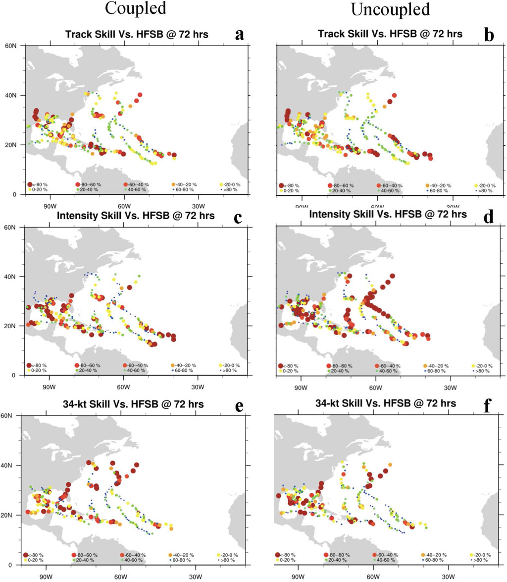
Figure 1. Spatial patterns in forecast skill (% difference relative to all HFSB forecasts, 2020–2022) for coupled (left) and uncoupled (right) cases at hour 72 of each forecast; largest dark red markers are for the lowest skill, dark blue for the most improved forecasts. Point locations indicate storm position at that forecast hour: (A, B) absolute track positional errors. (C, D) intensity as estimated by maximum sustained 10 m wind speed; and (E, F) radius of 34 kt winds (mean of the four quadrant-estimates).
Model verification statistics (Franklin, 2009; Jensen et al., 2023) are calculated for the coupled and uncoupled HAFS experiments over the entire coincident sample, which includes a total of 298 5-day forecasts by each model for 15 selected TCs during the 2020–2022 Atlantic hurricane seasons. The present study focuses on ocean impacts on tropical systems, so this sample set includes early-life cycle forecasts of invests - designated areas of disturbed weather - but excludes forecast cycles consisting primarily of periods when a TC had already undergone extratropical transition or was over land. Table 1 summarizes these comparative statistical analysis cases. The resulting sample size for the intensity metrics comprises 288 TC cases (forecasts of fully developed tropical cyclones) at forecast hour 0, and, excluding post-landfall, dissipation, or extratropical transition, 162 cases at forecast hour 120.
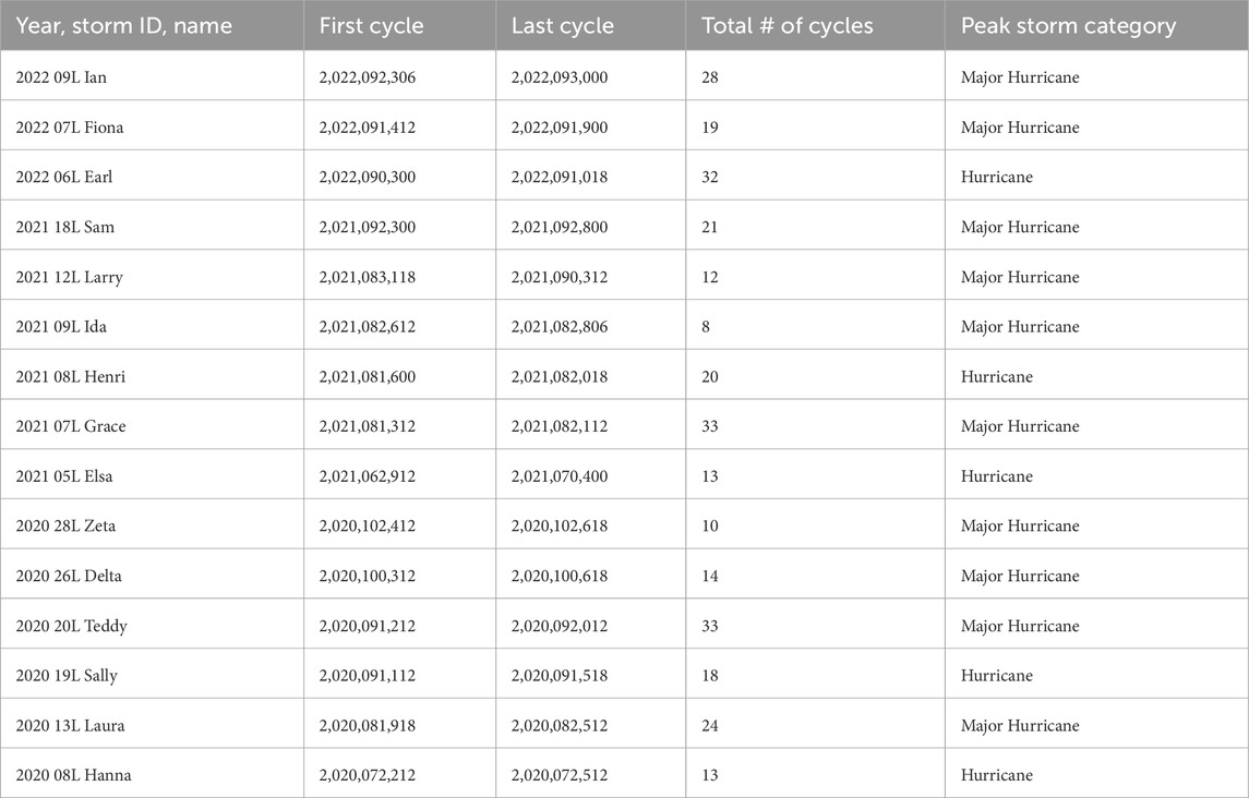
Table 1. All forecast cycles (298 total) analyzed for the present study.
The sample sizes for storm size metrics (e.g., 34 and 64 kt wind radii) were noticeably smaller because TCs in certain forecast cycles did not meet the criteria for those wind speeds. The quadrant-averaged statistics for R34, R50, and R64 presented below include zero values, which may have imparted some biases in the relative structure metrics between the two experiments. The authors thus further examined frequency distributions for the quadrants having both the smallest and largest radii for each metric, while excluding zero values.
For analysis of the contributions of individual storms to skill degradation in the comparative statistical analysis, we used the GROOT verification package (Ditchek et al., 2023). GROOT applies thresholds to three separate statistical metrics (mean absolute error or MAE skill, median absolute error skill, and frequency of superior performance) for each model performance metric, to objectively evaluate lead times with improvement or degradation that was either fully or marginally consistent across a sample. Thus, using this verification technique allows us to assess the robustness of differences in forecast skill. For the consistency metric and MAE skill for all metrics, retrospective forecasts of the HFSB for 2020–2022 were used as a baseline.
For the case studies, our aim was to identify TC characteristics which were enhanced or weakened in the uncoupled model relative to the coupled model, during and prior to significant TC intensity or structure change. Characteristics we considered included mid-level dry air intrusion, vertical wind shear (related to vertical TC alignment), and steering currents (related to translation speed), as well as differences in warm-core anomaly and surface wind fields. The definition of warm-core anomaly used here is the difference between the azimuthal mean potential temperature profile at each radial distance bin and the potential temperature profile averaged in the 200–300 km annulus from the center of the storm (Stern and Nolan, 2012; Zhang et al., 2020). The authors also analyzed coupled-versus-uncoupled differences in total (latent plus sensible) ASEF from the models, prior to TC structural changes. Wherever possible, we related these differences to changes in forecast SST that might be attributed to oceanographic processes (e.g., upper ocean mixing, upwelling, downwelling) forced by surface atmospheric conditions in the coupled model.
This paper first presents forecast verification statistics and statistical comparisons of SST and ASEF for all coupled and uncoupled forecasts which met NHC’s priority storm criteria. Based on these statistical results, the authors then select and analyze five individual TC forecasts in more detail: case studies that each demonstrate a different mechanism by which coupling a 3D dynamic ocean model can influence TC forecasts.
Figure 1 shows the spatial distribution of relative forecast skill between all coupled and uncoupled forecasts for several metrics at forecast hour 72, mapped to their corresponding forecast track location. The maps show that the sample of forecasts considered in this study spanned TCs which developed in the main TC development region of the central and eastern tropical north Atlantic, as well as those which developed or matured in the Caribbean Sea, Gulf of Mexico, and northwestern Atlantic. Figures 1A,B show that patterns of absolute positional error were similar between the two experiments. Figures 1C,D show the relative wind intensity forecast skill, and Figures 1E,F show relative forecast skill for mean 34 kt wind radii: Spatial patterns in both these latter sets of figures suggest that uncoupled forecasts often experience the greatest overintensification in regions of the ocean subject to the most variable SST, i.e., the subtropics of the North Atlantic and northern Gulf of Mexico. Interestingly, however, for a number of cases in the subtropics, structure (34 kt radius) skill in the coupled experiment (Figure 1E) was actually worse than that in uncoupled (Figure 1F).
When the authors compared absolute errors and biases between the coupled and uncoupled HFSB experiments (Figure 2), many of our results confirmed long-held hypotheses, but some of these analyses led to unexpected results. In contrast to previous work (see Introduction and Discussion), there were no statistically significant differences in absolute track errors (Supplementary Figure S3D), nor in along- or cross-track errors (figures not shown) between the coupled and uncoupled HFSB experiments.
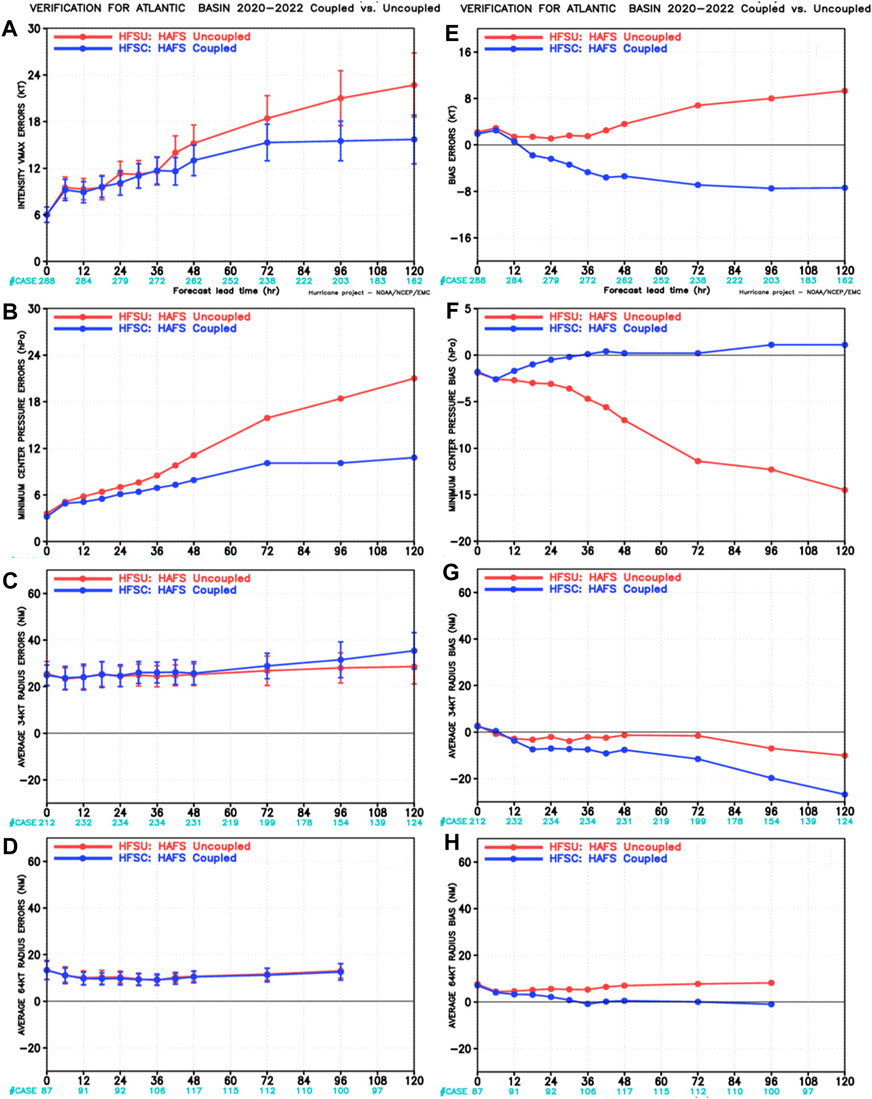
Figure 2. Forecast verification statistics for coupled (blue) and uncoupled (red) HFSB experiments relative to Best Track, comparing absolute errors (A–D) and biases (E–H) in maximum wind speed (A, E), minimum central pressure (B, F), 34 kt radius (C, G), and 64 kt radius (D, H), respectively. Case counts for each variable as a function of forecast hour are listed below the x-axis (cyan).
The dynamic ocean coupling reduced absolute intensity errors in forecasts of both maximum 10-m winds (Figure 2A) and minimum central pressure (Figure 2B). Beginning near forecast hour 36, the absolute intensity errors in maximum 10-m winds diverge and the uncoupled HFSB experiment performs much worse than the coupled HFSB. The difference is statistically significant at the 95% confidence level from about forecast hour 42 onward. Day 5 was an anomaly with indistinguishable median intensities between coupled and uncoupled, albeit it was also the day with the smallest sample size; however, uncoupled outliers were significantly more intense, with maximum surface winds as high as 180 kt compared with 147 kt for coupled (Supplementary Information, hereafter “SI”; Supplementary Figure S1). Furthermore, the uncoupled HFSB experiment results in a positive intensity bias at all forecast lead times with a maximum wind speed bias of nearly 8 kts at 5 days (Figure 2E). In contrast, the coupled HFSB experiments show a negative intensity bias after forecast hour 12 (Figure 2E), particularly noticeable from Day 2 onward (Supplementary Figure S1).
For intensity errors as measured by minimum central pressure, the uncoupled simulations produce large absolute errors characterized by a minimum central pressure bias that reaches −15 hPa at day 5. Interestingly, the coupled simulations perform better for minimum central pressure (Figure 2F) than for maximum 10-m winds (Figure 2E), with biases that are within 2 hPa of zero after day 1. When contrasted with the results in Figure 2E, the results in Figure 2F may show an inconsistency in the pressure-wind relationship in the coupled HFSB. It may also suggest that the distribution of kinetic energy in the coupled forecasts is wider than that in the actual TCs; we examine this possibility briefly in the analysis of differences in surface wind field sizes between the experiments below. Consideration of other potential explanations can also be found in the Discussion.
Regarding storm motion, if the present results had shown a significant negative bias in translation speed, this could be viewed as a possible cause of the concomitant negative bias in maximum 10 m winds for the coupled experiment: Over the open ocean, the dynamic ocean response represented in the coupled model is expected to have a greater impact on intensity for slower moving TCs (e.g., translation speeds of 10 kt or less; Halliwell et al., 2011). This expected impact is due to the development of the oceanic cold wake beneath the TC reducing the available energy at the air-sea interface. To examine this possibility, the authors compared biases in the storms’ median forecast motion (their translation speeds) between our coupled and uncoupled experiments, and found no statistically significant differences (Supplementary Figure S1) at the 95% confidence level; in fact, translation speeds among the coupled and uncoupled experiments and the Best Track were all statistically similar. This suggests that translation speed differences did not play a major role in intensity differences between the experiments.
In terms of the importance of the ocean to these results, it is notable that both experiments produced TCs with median translation speeds of approximately 10 kt (SI, Supplementary Figure S2A). In 50% of all forecasts, translation speeds were between 7 and 14 kt in days 1–3. These ranges of translation speeds suggest that the majority of cases in the present study would be impacted by coupling to a dynamic ocean (Halliwell et al., 2011). A few outliers were likely experiencing extratropical transition by days 4 and 5, with one forecast TC in the uncoupled experiment moving at 48 kt on day 5. Finally, we note that for both wind speed error biases (Supplementary Figure S1) and 34 kt radii in the largest quadrant (Supplementary Figure S2), later forecast hours of the uncoupled experiment show greater skew (distribution asymmetry) and heteroskedasticity (heterogeneity of variance) suggesting potentially lower predictability when compared with coupled HFSB.
The statistical analysis comparing structure metrics for the coupled and uncoupled experiments showed that average 34-kt radius errors were larger in the coupled HFSB experiment after day 3 (Figure 2C), while also resulting in negative bias, meaning the outer 34 kt wind field is much smaller in the coupled HFSB than uncoupled (Figure 2G). Average 64 kt radius errors are similar for both experiments, consistently near 15 km absolute error at all forecast lead times (Figure 2D). However, the coupled HFSB has a nearly zero bias in 64 kt radius, particularly after 36 h, while the uncoupled HFSB has a positive bias of nearly 10 km (Figure 2H). Therefore, the uncoupled HFSB produced an expanded 64-kt (hurricane strength) forecast wind field. Absolute errors in the radius of maximum winds (RMW, not shown) are similar between the experiments, with errors close to 20 km at all lead times. The bias in RMW (not shown) is also similar, with a positive bias of <10 km at all lead times. The uncoupled HFSB has a lower positive bias than the coupled experiment, highlighting the slight contraction of the RMW in the uncoupled experiment (not shown). The above summary highlights the different ways that dynamic ocean coupling (or lack thereof) can impact forecasts of storm structure and the associated wind field. Below, we consider metrics of vertical storm structure as well.
It was noted above that the coupled experiment produced negative wind speed biases after day 1, but very small minimum central pressure biases. These two findings appear to be inconsistent with a simplistic understanding of the wind-pressure relationship; as previously mentioned, one possible explanation for this inconsistency relates to wind field sizes. If that were the case, we might expect that the coupled model would overestimate the size of the TC; however, Figure 2G shows that the models, especially the coupled model, substantially underestimated the radii of 34 kt winds. Finally, comparing minimum and maximum 34 kt radii between the two experiments in days 1–4 (SI, Supplementary Figure S2), we note that the coupled forecasts were significantly smaller in both median (horizontal middle line) and 25th percentile (lower box boundaries) beginning with day 2. On day 5, the 34 kt radii for the uncoupled experiment became much larger, in fact, although this may simply be consistent with the more intense forecast TCs in that experiment. The authors note that minimum central pressure relates to the overall dynamic balance in a TC, whereas peak wind is not in balance, subject to turbulence, and therefore can be very noisy. The Discussion considers these results for wind intensity, minimum central pressure, and storm structure in more detail.
As a final part of our statistical analysis, we consider the processes by which the uncoupled HFSB contributed to more intense forecasts relative to the coupled HFSB in the present study. Figures 3A,B show that SST and ASEF within 100 km of the TC center, respectively, were consistently greater in the uncoupled experiment for all forecast days after day 1. Figure 3C shows peak warm-core anomaly temperatures, with peak coupled model temperature anomaly from individual 3 h coupled forecast periods on the y-axis and peak model temperature anomaly from the corresponding uncoupled forecast on the x-axis. While individual forecasts show outliers where the anomaly is greater for the coupled forecast (points above black 1-to−1 line) particularly for earlier forecast hours (days 1–4), by days 4 and 5 the great preponderance of points lie below the 1-to−1 line. There are a significant number of extreme points with anomaly > = 7 K from the uncoupled forecasts, with corresponding values for coupled near 0 K.
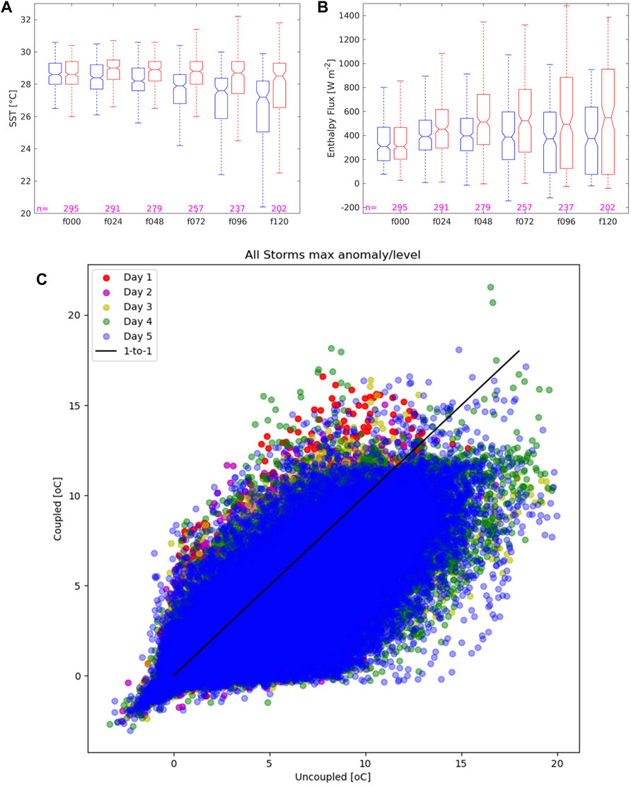
Figure 3. Boxplots of (A) SST and (B) ASEF averaged within 100 km annulus of TC center locations for the coupled (blue) and uncoupled (red) HFSB experiments as a function of forecast lead time. Case counts (magenta numbers) for each forecast lead time are listed along the x-axis. (C) Scatter plot of coupled versus uncoupled warm-core anomaly peak temperature across all model levels below 18 km. Color coding shows days into each forecast: red for forecast hours 0–23, magenta 24–47, yellow 48–71, green 72–95, blue 96–126.
Supplementary Figure S5 shows scatter plots of warm-core anomaly maximum for individual forecast days: on day 1, the relationship between uncoupled and coupled is essentially 1-to−1. By days 3 and 4, an increasing number of outliers are seen below the 1-to−1 line, showing the rapidly developing negative influence of a dynamic ocean on intensity. Also of note, however, are the continued cases of forecasts where we see the opposite: a greater warm-core anomaly for the coupled case, particularly on day 4. These cases likely include the evolution of open-ocean storms at higher latitudes, but also TCs that are interacting increasingly with land.
In this section, we analyze case studies of individual TC forecasts for five hurricanes: Larry, Earl, Fiona, Ian, and Elsa. Each case demonstrates a different physical process related to coupling that influences intensity forecasts. Figure 4 shows wind speed intensities, TC average SSTs (within 100 km of storm center), and TC average ASEF for forecast cycles of Larry, Earl, Fiona, and Ian. Figure 5 relates these patterns of SST and ASEF to the vertical structure of one representative example, Fiona. Figure 6 shows the influence of coupling on the near-storm environment of Elsa as it moved across the northwest Caribbean. Overall, the range of case studies presented below highlight different aspects of what is a diverse response of TCs to a dynamic ocean in coupled forecast models.
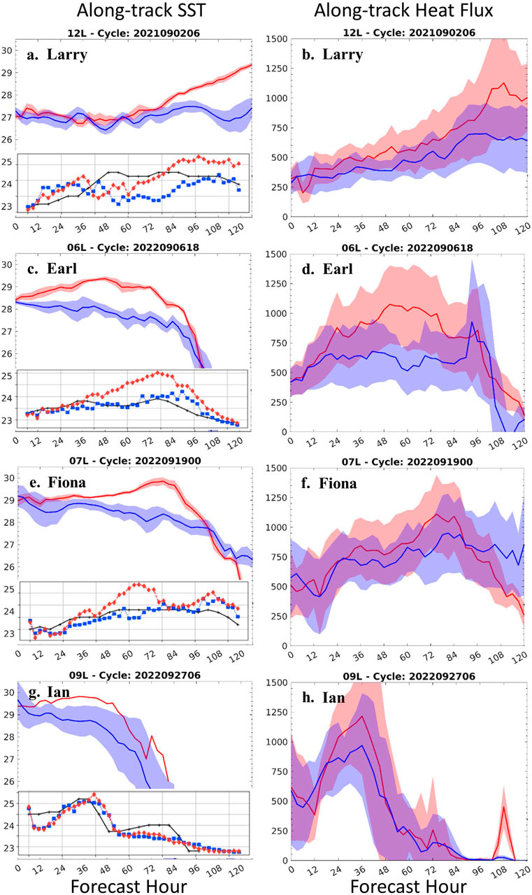
Figure 4. (Inset) Forecast wind intensity for coupled (blue) versus uncoupled (red) forecasts. (left) Mean (line) and +/- 1 STD (shading) of sea-surface temperature (SST) within 100 km of storm center for coupled and uncoupled forecasts. (right) Mean and +/- 1 STD of total air-sea enthalpy fluxes (ASEF) for coupled and uncoupled. Case studies shown are: ((A, B), 1st row) Hurricane Larry, 12L 2021, ((C, D), 2nd row) Hurricane Earl, 06L 2022, ((E, F), 3rd row) Hurricane Fiona, 07L 2022, and ((G, H), 4th row) Hurricane Ian, 09L 2022.
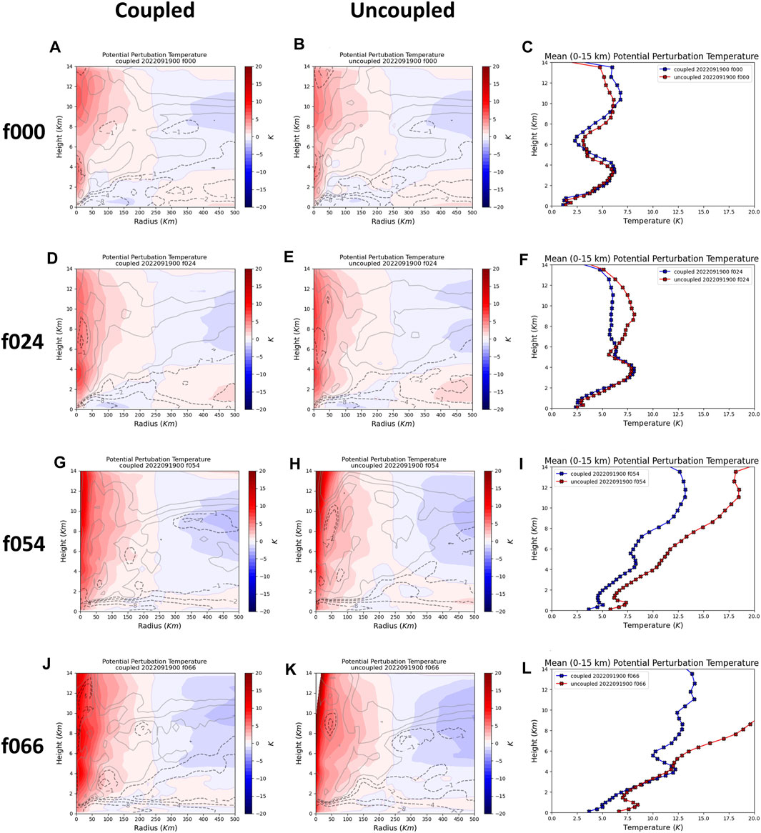
Figure 5. Evolution of warm-core anomaly (shading) and radial velocity (contours) for a forecast of Hurricane Fiona, highlighting the period of most rapid divergence between coupled (left panels, (A, D, G, J)) and uncoupled (middle panels, (B, E, H, K)) intensities (compare Figure 4E inset). Mean temperature anomalies at each model height between 0 and 15 km from the eye are shown in the right panels (c, f, i,l). Forecast hours shown are: (A,B, C) f000, (D,E, F) f024, (G,H, I) f054, and (J, K, L) f066.
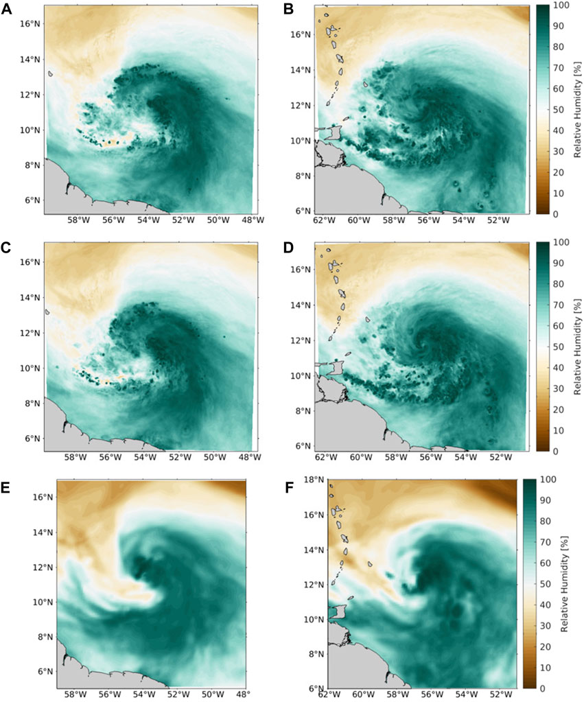
Figure 6. Relative humidity for forecasts of Hurricane Elsa averaged from 400 to 700 hPa for (A, B) HFSB coupled forecast, (C, D) uncoupled forecast, and (E, F) GFS analysis. The HFSB model output is from cycle 2,021,070,112 at two forecast hours, f012 (left) and f018 (right). The GFS analysis matches the valid time from HFSB.
An uncoupled forecast of Hurricane Larry initialized at 0600 UTC 2 September 2021, when both forecasts were moving west-northwest through the tropical Atlantic, showed intensification beginning on day 3 (Figure 4A, inset). This intensification coincided with the forecast TC’s passage over a region of higher SST (>27 C, Figure 4A); the higher SST resulted in an increase in ASEF (Figure 4B) that contributed directly to the uncoupled forecast intensification. In the case of Larry, this intensification ultimately verified versus Best Track (black line in Figure 4A inset) while the coupled forecast remained too weak, suggesting that coupling to the dynamic ocean model did not improve the skill for this forecast cycle.
Three of the remaining case studies (Earl, Fiona, Ian, below) follow this same broad pattern, but with the contrasting result that the coupled forecast shows significant improvement over the uncoupled as described below. An uncoupled forecast of Hurricane Earl for 2022–09–06 at 18Z showed substantial overintensification relative to both the coupled forecast and observations (Figure 4C, inset). The TC in the uncoupled forecast experienced warm SSTs throughout the period of overintensification (Figure 4C), and significantly greater ASEF particularly during day 3 (Figure 4D).
A forecast for Fiona (Figures 4E,F), initialized on 2022–09–19 at 00Z, showed a very similar pattern of unverified overintensification (Figure 4E, inset) and enhanced SST (Figure 4E) in the uncoupled forecast at least on days 2–3. ASEF was also greater in the uncoupled case (Figure 4F), albeit differences were less in day 2, suggesting the near-storm environment may have also played a role in differences between coupled and uncoupled forecasts for Fiona (see Elsa case below). Further analysis of the vertical atmospheric structure of Fiona during intensification is summarized below.
Forecasts for Hurricane Ian (Figures 4G,H), initialized on 2022–09–27 at 06Z, show early spin-down (potentially related to atmospheric data assimilation, see Annane and Gramer, 2022); but just prior to Florida landfall, around forecast hour 42, the uncoupled case showed increases in intensity (Figure 4G, inset), SST (Figure 4G), and ASEF (Figure 4H) that did not verify, as compared to the coupled forecast.
For one of the case studies, Fiona, we discuss the evolution of relative heat and moisture concentration in the TC core as represented by the warm-core anomaly (Figure 5, see Methods). At forecast initialization, both the coupled (Figure 5A) and uncoupled storms (Figure 5B) have very similar vertical structures. The structure of the warm-core anomaly evolves through time coincident with the changes in ASEF (Figure 4F). As we have seen in Figure 4, differences in the time evolution of the SST and ASEF correlate well with differences in the intensity forecast between the coupled and uncoupled experiments. This is clearly seen from hours 12 to 24 (Figure 4) when the SST, the ASEF, and the intensity all start to diverge. Beyond this time, the uncoupled case continues to intensify along with a further divergence in SST and ASEF. In terms of the vertical structure at t hour 24 (Figures 5D,E), the temperature anomaly is similar in the lower 6 km for both cases, but above this height the uncoupled case begins to show an enhanced warm core, consistent with more rapid intensification beginning at that hour.
By hour 54, the center of the warm-core anomaly for the uncoupled case (Figure 5H) has increased in height and intensified significantly relative to the coupled (Figure 5G); at a height of 11 km, this anomaly difference amounts to 8 K (Figure 5I). By hour 66, when the uncoupled case has reached its maximum intensity, this difference is even greater (Figures 5J,K), with anomaly differences at heights above 10 km of more than 10 K (Figure 5L). In general, at hour 66, the temperature anomalies differ notably in the bottom 2 km and above 6 km (Figure 5). This result demonstrates that the presence of a dynamic ocean can strongly affect the temperature and humidity structure of a storm far above the boundary layer.
The final case study, Elsa, initialized at 1200 UTC 01 July 2021, is an example of the indirect influence of ocean coupling on TC intensity, as mediated through differences in the near-storm environment between coupled and uncoupled experiments. Unlike in the Earl case, differences in footprint SST and ASEF for Elsa were not substantial (Supplementary Figure S6) during the period of anomalous overintensification in the uncoupled forecast (hours 24–60, Supplementary Figure S4E). And differences in footprint SST between coupled and uncoupled were actually mixed throughout that period of rapid intensification in the uncoupled run. This suggests that something other than the development of a cold wake caused the intensity of the coupled forecast for Elsa to verify better in days 2 and 3 of the forecast.
Figure 6 shows the mid-level (400–700 hPa) mean relative humidity in the coupled and uncoupled runs, both at hour 12 when the two intensity forecasts were very similar, and at hour 18 when they began to diverge substantially (Supplementary Figure S4). Also shown is the GFS Analysis, which included moisture soundings. These figures confirm that a major contributor to the weakening of the TC in the coupled forecast was mid-tropospheric dry air intrusion; this feature did not arise in the uncoupled forecast, even though both the storm intensity and the near-storm mid-tropospheric moisture at 12 h were nearly identical (Figures 6A,C). As the only configuration difference between the two experiments was the dynamic ocean response in the coupled experiment, this case demonstrates that ocean coupling can modify the broader environment of the TC in ways that can impact intensity forecasts.
The present study examined forecasts of TCs from the 2020–2022 Atlantic hurricane seasons produced by NOAA’s operational HFSB forecasting system, which couples the FV3 model (initialized using vortex modification and atmospheric data assimilation) to the HYCOM ocean model (initialized from data-assimilating nowcasts of the global RTOFS). The analysis period of 2020–2022 allowed the researchers to leverage the nearly complete archive of retrospective forecasts from HFSB for those years. However, this period included both a highly active (2020) and two less active seasons (2021, 2022) for Atlantic TCs, and included periods both with and without the influence of important external factors, such as El Niño-Southern Oscillation (ENSO) variability. The authors therefore believe that the present study encompasses a large enough sample to capture between-season variability, and that many of our conclusions will find more general applicability in the future.
In order to examine the effects of coupling on forecasts, we selected NHC-priority TCs for which the coupled HFSB produced relatively small errors in forecast track during these three seasons. For these storms, we produced coincident uncoupled forecasts using an atmospheric configuration identical to HFSB, except that the dynamically coupled HYCOM was replaced by the NSST product. NSST superposes near-surface (“foundation”) sea temperature from the GFS modeling system at initialization time, with a simple diurnal model of upper ocean temperature variability (a “static ocean”).
The uncoupled forecasts produced significant negative biases in minimum central pressure, and significant positive biases in peak winds and structure statistics, consistent with many prior findings (see Introduction). The coupled forecasts, on the other hand, produced overall skillful minimum central pressure (e.g., Schade et al., 1994) and TC inner core structure, but with overly small TC outer structure (negative bias in 34 kt wind radii) and overly weak maximum winds (negative bias in 10 m surface wind) relative to observations. We noted that the coupled experiment did provide more reliable information about inner storm structure, even though it was less skillful than the uncoupled experiment at forecasting outer storm structure. (In particular, R64 and RMW had lower biases coupled vs uncoupled, while the quadrant-mean R34 negative biases noted above in our coupled experiment, on the other hand, were largely due to lower medians and 25th-percentiles in the largest quadrant at days 2–5.) This is in contrast to earlier findings regarding coupling and outer wind field size (Guo et al., 2020; Pun et al., 2021). Forecasts with too small an outer wind field, as is the case with our coupled experiment, can reduce reliability in forecasting hazards (waves, storm surge), so the mechanisms underlying this finding are worth further study. Additional analysis may also shed light on the impact of coupling on the radii of 50 kt winds specifically, which are important for wind hazard forecasting (Powell and Reinhold, 2007).
Our results for pressure and structure are consistent with previously identified biases in HFSB (Hazelton et al., 2024) as well as other models (Takaya et al., 2010). This combination of results may simply be a matter of pressure being in balance in the atmospheric model, while peak wind is not, thereby making peak wind less predictable. However, it is also possible that these results for pressure, peak wind, and storm size suggest an inconsistency in the way the pressure-wind gradient relationship is modeled in HFSB. They may, for example, point to an issue with thermodynamic-mechanical energy conversion, e.g., in the atmospheric planetary boundary layer physics.
On the other hand, the results for wind intensity and size may also suggest that, in some cases, the ocean modeled in HFSB responds more vigorously than the real ocean to the TC above it. Additional research is called for to help distinguish these potential causes for the observed discrepancies. Finally, bias differences in 34 kt wind radii between coupled and uncoupled forecasts could suggest issues with the definitions used for wind radius estimates by the tracking software in HFSB as compared to those used by the NHC; different handling of missing R34 quadrant estimates, for example, (see Results above), may still account for some part, albeit not all, of the observed bias. We believe these hypotheses to be worthy of further investigation.
In particular, for future work we would suggest isolating and removing the effects of any methodological differences in wind radius estimation between NHC best track and the model tracker. For residual biases in size between the coupled and uncoupled forecasts, we would then recommend investigating as follows. Tangential wind evolution has been found to be sensitive to the storm-relative location of ASEF as well as convective heating (e.g., Maclay et al., 2008; Musgrave et al., 2012). Enthalpy redistribution within the RMW tends to confine radial velocity response to the near center, directly contributing to intensity increase. Heating and enthalpy redistribution outside the RMW, on the other hand, tends to increase storm size. For a future study therefore, we would propose comparing ASEF and convective heating within the RMW vs outside of it, particularly for forecasts where coupled vs uncoupled experiments show significant differences in storm size change.
Another new finding of the present study was the minimal differences in track between coupled and uncoupled experiments across multiple Atlantic seasons. This finding expands upon some earlier, more limited studies (Chen et al., 2010), but contradicts others (e.g., Holt et al., 2011; Sun et al., 2017; Chen et al., 2023) that show improvements to TC track with model coupling. One hypothesis to explain this is that these differences may in part be due to the inclusion criteria for storms in our experiment. In particular, the present study began with coupled forecasts that had low track error (see above); a more complete sample of all TC forecasts for an extended period (multiple seasons) may well reproduce earlier results on the improvement of track skill due to coupling.
A further original finding of the present study was the differing spatial patterns of forecast error/skill between coupled and uncoupled experiments, in particular, for intensity (Figures 1C,D) and size (R34; Figures 1E,F). The result for intensity expands previous findings from the western Pacific (Mogensen et al., 2017) into storms in the Atlantic basin; the R34 result appears to be wholly novel. In addition, we noted in the present study that error distributions for wind speed and R34 radii deviated further from a normal (Gaussian) distribution in the uncoupled experiment. This suggests that the coupled experiment offers greater predictability of intensity and structure than the uncoupled.
In line with the many atmospheric forecast differences noted above between the experiments, we found that waters beneath the storm were generally warmer and provided more enthalpy in the uncoupled experiment after the first day, particularly for those TCs over the deep ocean. Consistent with this warmer SST and greater ASEF, air in the inner storm core for these cases was warmer and more moist (deeper, warmer WCA) in the uncoupled experiment as well after day 1. This latter result is novel for the Atlantic in the sense that it shows coincident evolution of cooler SST, lower ASEF, and shallower WCA in the dynamic ocean case. This result confirms earlier results in other ocean basins (Srinivas et al., 2016; Mohan et al., 2022). The coincidence of these effects links the coupled experiment to slower and more skillful forecasts of TC intensification, in particular for central pressure. There were also some forecasts that showed greater WCA in the coupled case. These counterexamples are consistent with the fact that other processes besides cooling SST also drive vertical structure change; future research should focus on characterizing and distinguishing these factors from the effects of ocean cooling directly beneath the storm (see discussions of the Fiona, Ian, and Elsa case studies below).
This work presented individual forecasts of storms where the coupling produces a clear forecasting advantage, e.g., Ian. For this case, the reduction in ASEF in the coupled forecast occurs over the west Florida shelf, leading us to hypothesize that the balance between vertical ocean mixing and shallow-ocean processes (in this case, coastal downwelling, Gramer et al., 2022) might have played an important role in the rate of intensification in this TC just before landfall. The ocean dynamics underlying this and similar TC-shelf interaction cases are something we hope to examine in much more detail with future work.
It is also of note, however, that the improved pressure forecast performance in coupled HFSB as compared to uncoupled is dominated in our sample by three large, open-ocean storms: Earl, Fiona, and Teddy (SI, Supplementary Figure S3B). These same three storms (together with Delta, Supplementary Figure S3A), also dominated differences in wind intensity. When forecast cycles for just these three storms were removed from our analysis (figures not shown), the differences in forecast skill between coupled and uncoupled were far less substantial. This, together with our findings from individual case studies (e.g., Ian above, and Larry, discussed below), suggests that coupling effects are nonlinear and that coupling to a dynamic ocean does not always produce better results. This may often be the case for smaller or faster-moving TCs, but fast-moving TCs were few in the sample analyzed here (Supplementary Figure S2A). However, regardless of storm motion, coupling in HFSB does tend to improve forecasts for storms that are in environments liable to produce substantial intensification, such as the open subtropical ocean (as is the case with Earl, Fiona, Teddy; Supplementary Figure S4). One possible reason for this is that in coastal storms, the coupled ocean model may not always reproduce the coastal ocean circulation appropriately; the coastal storms in our sample may also intensify more quickly, leaving less time for ocean impacts to be felt. We again recommend further studies to examine these questions.
This paper discusses five individual case studies. The first, as mentioned above, is an important counterexample to the general argument of the paper: an uncoupled forecast of Larry produced a more intense TC but was also more skillful than the coupled. Larry was a relatively slow moving TC in both experiments and in the observations, during the 5 days of this forecast. The Larry forecast suggests that other factors besides storm size or translation speed, including non-linear effects that result from a combination of factors, should be considered in future analyses of coupled TC forecasts.
The coupled forecasts for the Earl, Fiona, and Ian case studies followed the pattern of cooler SST, lower ASEF, and slower, more physical intensification set out in the full statistical results above. Earl in particular provided a good example of the general linkage between cooling and intensity seen in Figure 2 and Figure 3. The differences in ASEF between the coupled and uncoupled Fiona forecasts were less marked, while Ian showed evidence of coastal and shelf ocean interaction for which coupling was also important. For Fiona, the somewhat weaker distinction in ASEF between the coupled and uncoupled forecasts also suggested that ocean coupling played some role in modifying the wider environment around the storm as well. Further work elucidating this indirect effect of coupling may be valuable (see below). For Ian, the pattern of difference between coupled and uncoupled played out while the storm was largely interacting with the shallow rather than the deep ocean, suggesting that coupling is important for forecasting landfalling cases as well (e.g., Gramer et al., 2022).
For both Earl and Fiona in the open ocean, coupling produced ocean cooling near the inner core of the TC (Figure 4) and improved forecasts for intensity and structure (Supplementary Figure S4). For cases where SST response beneath the core is strong, the link between ocean dynamics and reduced warm-core anomaly and ultimately reduced intensity is clear. For a case like Fiona, the differences in SST and ASEF between the coupled and uncoupled cases, while not as strong, still correlate well with the differences in intensity between the experiments (Figure 4). In particular, we see with Fiona that the WCA (Figure 5) evolved in lockstep with changes in the ASEF over time. This case, while complex, nonetheless illustrates the result noted in our statistical analysis above, that the presence of a dynamic ocean may strongly affect the temperature structure of a storm far beyond the boundary layer.
As Hurricane Ian crossed the west Florida shelf just prior to landfall, HFSB coupling produced a forecast which avoided a notable overintensification seen in the uncoupled forecast. For Hurricane Larry, the ocean coupling degraded the forecast relative to the uncoupled experiment. We hypothesize that this case might indicate that coupling can reinforce issues in the atmospheric forecast related to other causes, e.g., atmospheric physics parameterization. This might suggest a need to tune physics parameterizations simultaneously in both the ocean and atmosphere, a hypothesis worthy of further research.
For our final case study, Elsa, the coupled intensity forecast was better than the uncoupled, apparently because of differences in the near-storm environment rather than the inner TC core, i.e., the intrusion of mid-tropospheric dry air. Although timing and extent of the dry-air intrusion were not perfectly forecast in this case study, the coupled model reproduced a dry slot near Elsa’s core that was apparent in GFS analysis, while the uncoupled model failed to do so. As the storm moved across the northeast Caribbean, the improved forecast of this dry slot in turn allowed the coupled model to forecast a reduced intensity relative to uncoupled, which was ultimately verified. One possible explanation for this is that the uncoupled forecast had already begun to over-intensify by hour 12, shielding the core from dry-air intrusion in a way that did not verify with the real TC. As noted in our Introduction, literature has discussed the impact of ocean coupling on large-scale climate conditions related to TC activity (Cai et al., 2019; Li and Sriver, 2019) and on TC-TC interaction (Alaka et al., 2020). The present study, however, is the only published result we are familiar with that attributes intensity changes to coupling-related changes in the near-TC environment.
These case studies by no means represent an exhaustive analysis of all intensification processes in all coupled HFSB forecasts, but they demonstrate some of the mechanisms by which a dynamic ocean can be directly linked with intensity and structure change in TC forecasts. Together with the statistical analyses presented in Section 3.1, these results may serve as a guide for modelers and researchers in future efforts to improve coupled TC models. The authors therefore hope that the present study will ultimately help to point future research in fruitful directions.
The present study directly addresses the following themes within the focus of Frontiers Earth Sciences, and specifically the special issue on “Tropical Cyclone Modeling and Prediction: Advances in Model Development and Its Applications”: Model development (two distinct configurations of a TC modeling system are utilized and examined); Air-sea interaction (in particular, the mechanisms by which air-sea interaction directly impact coupled TC forecasts), and Model track and intensity verification (including methods for evaluating the ocean component of coupled TC modeling systems). The paper further presents results of novel or recently developed evaluation tools for TC modeling systems (100-km storm-centered footprint averages and standard deviations of key model variables; warm-core anomaly comparisons between experiments; the Ditchek GROOT package).
The datasets presented in this study can be found in online repositories. The names of the repository/repositories and accession number(s) can be found in the article/Supplementary Material.
LG: Writing–review and editing, Writing–original draft, Visualization, Validation, Software, Project administration, Methodology, Investigation, Formal Analysis, Data curation, Conceptualization. JS: Writing–original draft, Validation, Software, Methodology, Investigation, Formal Analysis, MA: Writing–original draft, Validation, Software, Methodology, Investigation, Formal Analysis. H-SK: Writing–original draft, Validation, Software, Methodology, Formal Analysis, Conceptualization.
The author(s) declare that financial support was received for the research, authorship, and/or publication of this article. Funding from NOAA projects GR013873 and GR021701 (A. Hazelton, PI) supported LJG in performance of the experiments and preparation of this manuscript.
LG gratefully acknowledges overall research guidance from G. Alaka and F. Marks, NOAA-HRD, who also provided helpful internal review of the manuscript prior to submission. Initial conceptualization for this study came out of very helpful conversations between LG and J. A. Zhang of CIMAS and NOAA-HRD, as well as LG and H-SK. Several ocean-related statistical evaluation metrics were first suggested by HSK. In addition, the final submission of the paper was greatly enhanced by the comments of M. DeMaria, particularly with regard to R34, and the comments of an reviewer. Concision and clarity of the manuscript were greatly improved by consultations with the University of Miami Writing Center, particularly A. Mann, R. Klass, and L. Albritton.
The authors declare that the research was conducted in the absence of any commercial or financial relationships that could be construed as a potential conflict of interest.
All claims expressed in this article are solely those of the authors and do not necessarily represent those of their affiliated organizations, or those of the publisher, the editors and the reviewers. Any product that may be evaluated in this article, or claim that may be made by its manufacturer, is not guaranteed or endorsed by the publisher.
The Supplementary Material for this article can be found online at: https://www.frontiersin.org/articles/10.3389/feart.2024.1418016/full#supplementary-material
Agrenich, E. A. (1984). Effect of sea surface temperature on the trajectory of a tropical cyclone. Soviet Meteorology Hydrology 4, 2631.
Alaka, G. J., Zhang, X. J., Gopalakrishnan, S. G., Goldenberg, S. B., and Marks, F. D. (2017). Performance of basin-scale HWRF tropical cyclone track forecasts. Weather Forecast. 32 (3), 1253–1271. doi:10.1175/waf-d-16-0150.1
Alaka Jr, G. J., Sheinin, D., Thomas, B., Gramer, L., Zhang, Z., Liu, B., et al. (2020). A hydrodynamical atmosphere/ocean coupled modeling system for multiple tropical cyclones. Atmosphere 11 (8), 869. doi:10.3390/atmos11080869
Annane, B., and Gramer, L. (2024). Influence of CyGNSS L2 wind data on tropical cyclone analysis and forecasts in the coupled HAFS/HYCOM system. Earth Sci. Special Ed.
Bender, M. A., Ginis, I., and Kurihara, Y. (1993). Numerical simulations of tropical cyclone-ocean interaction with a high-resolution coupled model. J. Geophys. Res. Atmos. 98, 23245–23263. doi:10.1029/93JD02370
Bleck, R., Halliwell, G. R., Wallcraft, A. J., Carroll, S., Kelly, K., and Rushing, K. (2002). HYbrid Coordinate Ocean Model (HYCOM) user’s manual: details of the numerical code. HYCOM, 211pp.
Cai, W., Wu, L., Lengaigne, M., Li, T., McGregor, S., Kug, J. S., et al. (2019). Pantropical climate interactions. Science 363, eaav4236. doi:10.1126/science.aav4236
Chang, S. W., and Anthes, R. A. (1979). The mutual response of the tropical cyclone and the ocean. J. Phys. Oceanogr. 9, 128–135. doi:10.1175/1520-0485(1979)009<0128:TMROTT>2.0.CO;2
Chang, S. W., and Madala, R. V. (1980). Numerical simulation of the influence of sea surface temperature on translating tropical cyclones. J. Atmos. Sci. 37, 2617–2630. doi:10.1175/1520-0469(1980)037<2617:NSOTIO>2.0.CO;2
Chassignet, E. P., Hurlburt, H. E., Smedstad, O. M., Halliwell, G. R., Hogan, P. J., Wallcraft, A. J., et al. (2007). The HYCOM (HYbrid Coordinate Ocean Model) data assimilative system. J. Mar. Syst. 65, 60–83. doi:10.1016/j.jmarsys.2005.09.016
Chen, S., Campbell, T. J., Jin, H., Gaberšek, S., Hodur, R. M., and Martin, P. (2010). Effect of two-way air–sea coupling in high and low wind speed regimes. Mon. Weather Rev. 138, 3579–3602. doi:10.1175/2009MWR3119.1
Chen, Y., Wei, Y., Zheng, Y., Liu, Q., Sun, L., Zhao, B., et al. 2023. Numerical investigation of Air-Sea coupling to the track and intensity of landfalling tropical cyclones in the south China sea. doi:10.21203/rs.3.rs-3723682/v1
Cione, J. J., and Uhlhorn, E. W. (2003). Sea surface temperature variability in hurricanes: implications with respect to intensity change. Mon. Weather Rev. 131 (8), 1783–1796. doi:10.1175//2562.1
Davis, C., Wang, W., Chen, S. S., Corbosiero, K., DeMaria, M., Dudhia, J., et al. (2008). Prediction of landfalling hurricanes with the advanced hurricane WRF model. Mon. Wea. Rev. 136, 1990–2005. doi:10.1175/2007mwr2085.1
Ditchek, S. D., Sippel, J. A., Marinescu, P. J., and Alaka, G. J. (2023). Improving best track verification of tropical cyclones: a new metric to identify forecast consistency. Weather Forecast. 38 (6), 817–831. doi:10.1175/waf-d-22-0168.1
Ek, M. B., Mitchell, K. E., Lin, Y., Rogers, E., Grunmann, P., Koren, V., et al. (2003). Implementation of noah land surface model advances in the national centers for environmental prediction operational mesoscale Eta model. J. Geophys. Res. 108, 2002JD003296. doi:10.1029/2002JD003296
Franklin, J. L. (2009). 2008 National Hurricane Center forecast verification report. China: NOAA, 71. Available at: http://www.nhc.noaa.gov/verification/pdfs/Verification_2008.pdf.
Garraffo, Z. D., Cummings, J. A., Paturi, S., Iredell, D., Spindler, T., Balasubramanian, B., et al. (2020). Research activities in Earth system modelling. Programme Geneva: World Climate Research.
Gramer, L. J., Zhang, J. A., Alaka, G., Hazelton, A., and Gopalakrishnan, S. (2022). Coastal downwelling intensifies landfalling hurricanes. Geophys. Res. Lett. 49, e2021GL096630. doi:10.1029/2021gl096630
Guo, T., Sun, Y., Liu, L., and Zhong, Z. (2020). The impact of storm-induced SST cooling on storm size and destructiveness: results from atmosphere-ocean coupled simulations. J. Meteorol. Res. 34, 1068–1081. doi:10.1007/s13351-020-0001-2
Halliwell, G. R., Shay, L. K., Brewster, J. K., and Teague, W. J. (2011). Evaluation and sensitivity analysis of an ocean model response to Hurricane Ivan. Mon. weather Rev. 139 (3), 921–945. doi:10.1175/2010mwr3104.1
Han, J., and Bretherton, C. S. (2019). TKE-based moist eddy-diffusivity mass-flux (EDMF) parameterization for vertical turbulent mixing. Weather and Forecasting 34, 869–886. doi:10.1175/WAF-D-18-0146.1
Hazelton, A., Alaka, G. J., Gramer, L., Ramstrom, W., Ditchek, S., Chen, X. M., et al. (2023). 2022 real-time hurricane forecasts from an experimental version of the Hurricane Analysis and Forecast System (HAFSv0.3S). Front. Earth Sci. 11, 17. doi:10.3389/feart.2023.1264969
Hazelton, A., Chen, X., Alaka, G. J., Alvey, G. R., Gopalakrishnan, S., and Marks, F. (2024). Sensitivity of HAFS-B tropical cyclone forecasts to planetary boundary layer and microphysics parameterizations. Weather Forecast. 39, 655–678. doi:10.1175/WAF-D-23-0124.1
Hazelton, A., Zhang, Z., Liu, B., Dong, J. L., Alaka, G., Wang, W. G., et al. (2021). 2019 atlantic hurricane forecasts from the global-nested hurricane analysis and forecast system: composite statistics and key events. Weather Forecast. 36 (2), 519–538. doi:10.1175/waf-d-20-0044.1
Heffner, D. M., Subrahmanyam, B., and Shriver, J. F. (2008). Indian ocean rossby waves detected in HYCOM sea surface salinity. Geophys. Res. Lett. 35 (3). doi:10.1029/2007GL032760
Holt, T. R., Cummings, J. A., Bishop, C. H., Doyle, J. D., Hong, X., Chen, S., et al. (2011). Development and testing of a coupled ocean–atmosphere mesoscale ensemble prediction system. Ocean. Dyn. 61, 1937–1954. doi:10.1007/s10236-011-0449-9
Iacono, M. J., Delamere, J. S., Mlawer, E. J., Shephard, M. W., Clough, S. A., Collins, W. D., et al. (2008). Radiative forcing by long-lived greenhouse gases: Calculations with the AER radiative transfer models. J. Geophys. Res. 113, 2008JD009944. doi:10.1029/2008JD009944
Jaimes, B., and Shay, L. K. (2015). Enhanced wind-driven downwelling flow in warm oceanic eddy features during the intensification of Tropical Cyclone Isaac (2012): observations and theory. J. Phys. Oceanogr. 45 (6), 1667–1689. doi:10.1175/jpo-d-14-0176.1
Jaimes, B., Shay, L. K., and Halliwell, G. R. (2011). The response of quasigeostrophic oceanic vortices to tropical cyclone forcing. J. Phys. Oceanogr. 41 (10), 1965–1985. doi:10.1175/jpo-d-11-06.1
Jaimes, B., Shay, L. K., and Uhlhorn, E. W. (2015). Enthalpy and momentum fluxes during Hurricane Earl relative to underlying ocean features. Mon. Weather Rev. 143 (1), 111–131. doi:10.1175/mwr-d-13-00277.1
Jensen, T., Prestopnik, J., Soh, H., Goodrich, L., Brown, B., Bullock, R., et al. (2023). The MET version 11.1.0 user’s guide. Developmental testbed center. Available at: https://github.com/dtcenter/MET/releases.
Kara, B., Wallcraft, J., and Hurlburt, H. E. (2005). A new solar radiation penetration scheme for use in ocean mixed layer studies: an application to the Black Sea using a fine-resolution Hybrid Coordinate Ocean Model (HYCOM). J. Phys. Oceanogr. 35 (1), 13–32. doi:10.1175/jpo2677.1
Kara, B., Wallcraft, J., Martin, P. J., and Chassignet, E. P. (2008). Performance of mixed layer models in simulating SST in the equatorial Pacific Ocean. J. Geophys. Research-Oceans 113 (C2), 16. doi:10.1029/2007jc004250
Khain, A., and Ginis, I. (1991). The mutual response of a moving tropical cyclone and the ocean. Contrib. Atmos. Phys. 64, 125–141.
Kim, H.-S., Liu, B., Thomas, B., Rosen, D., Wang, W., Hazelton, A., et al. (2022a). Ocean component of the first operational version of hurricane analysis and forecast system: HYbrid coordinate Ocean model (HYCOM). Submitt. this Front. Earth Sci. Special Ed. doi:10.3389/feart.2024.1399409
Kim, H. S., Lozano, C., Tallapragada, V., Iredell, D., Sheinin, D., Tolman, H. L., et al. (2014). Performance of ocean simulations in the coupled HWRF-HYCOM model. J. Atmos. Ocean. Technol. 31 (2), 545–559. doi:10.1175/jtech-d-13-00013.1
Kim, H.-S., Meixner, J., Thomas, B., Reichl, B. G., Liu, B., Mehra, A., et al. (2022b). Skill assessment of NCEP three-way coupled HWRF-HYCOM-WW3 modeling system: hurricane laura case study. Weather Forecast. 37 (8), 1309–1331. doi:10.1175/waf-d-21-0191.1
L’Hégaret, P., Duarte, R., Carton, X., Vic, C., Ciani, D., Baraille, R., et al. (2015). Mesoscale variability in the Arabian Sea from HYCOM model results and observations: impact on the Persian Gulf Water path. Ocean Sci. 11 (5), 667–693.
Large, W. G., McWilliams, J. C., and Doney, S. C. (1994). Oceanic vertical mixing - a review and a model with a nonlocal boundary-layer parameterization. Rev. Geophys. 32 (4), 363–403. doi:10.1029/94rg01872
Le Hénaff, M., Domingues, R., Halliwell, G., Zhang, J. A., Kim, H.-S., Aristizabal, M., et al. (2021). The role of the Gulf of Mexico ocean conditions in the intensification of Hurricane Michael (2018). J. Geophys. Res. Oceans 126 (5), e2020JC016969. doi:10.1029/2020jc016969
Leipper, D. F., and Volgenau, D. (1972). Hurricane heat potential of the Gulf of Mexico. J. Phys. Oceanogr. 2 (3), 218–224. doi:10.1175/1520-0485(1972)002<0218:hhpotg>2.0.co;2
Li, H., and Sriver, R. L. (2019). Impact of air–sea coupling on the simulated global tropical cyclone activity in the high-resolution Community Earth System Model (CESM). Clim. Dyn. 53, 3731–3750. doi:10.1007/s00382-019-04739-8
Lin, S. J. (2004). A “vertically Lagrangian” finite-volume dynamical core for global models. Mon. Weather Rev. 132 (10), 2293–2307.
Lybarger, N. D., Newman, K. M., and Kalina, E. A. (2023). Diagnosing hurricane barry track errors and evaluating physics scalability in the UFS short-range weather application. Atmosphere 14 (9), 1457. doi:10.3390/atmos14091457
Maclay, K. S., DeMaria, M., and Vonder Haar, T. H. (2008). Tropical cyclone inner core kinetic energy evolution. Mon. Wea. Rev. 136, 4882–4898. doi:10.1175/2008mwr2268.1
Metzger, E. J., Smedstad, O. M., Thoppil, P. G., Hurlburt, H. E., Cummings, J. A., Wallcraft, A. J., et al. (2014). US navy operational global ocean and arctic ice prediction systems. Oceanography 27, 32–43.
Mogensen, K. S., Magnusson, L., and Bidlot, J.-R. (2017). Tropical cyclone sensitivity to ocean coupling in the ECMWF coupled model. J. Geophys. Res. Oceans 122 (5), 4392–4412. doi:10.1002/2017jc012753
Mohan, P. R., Srinivas, C. V., Yesubabu, V., Rao, V. B., Murthy, K. V., and Venkatraman, B. (2022). Impact of SST on the intensity prediction of extremely severe tropical cyclones fani and amphan in the bay of bengal. Atmos. Res. 273, 106151. doi:10.1016/j.atmosres.2022.106151
Musgrave, K. D., Taft, R. K., Vigh, J. L., McNoldy, B. D., and Schubert, W. H. (2012). Time evolution of the intensity and size of tropical cyclones. J. Adv. Model. Earth Syst. 4, M08001. doi:10.1029/2011ms000104
Pottapinjara, V., and Joseph, S. (2022). Evaluation of mixing schemes in the HYbrid coordinate Ocean Model (HYCOM) in the tropical Indian ocean. Ocean. Dyn. 72 (5), 341–359. doi:10.1007/s10236-022-01510-2
Powell, M. D., and Reinhold, T. A. (2007). Tropical cyclone destructive potential by integrated kinetic energy. Bull. Am. Meteorological Soc. 88 (4), 513–526. doi:10.1175/bams-88-4-513
Pun, I.-F., Knaff, J. A., and Sampson, C. R. (2021). Uncertainty of tropical cyclone wind radii on sea surface temperature cooling. J. Geophys. Res. Atmos. 126, e2021JD034857. doi:10.1029/2021JD034857
Putman, W. M., and Lin, S. J. (2009). “A finite-volume dynamical core on the cubed-sphere grid,” in Numerical Modeling of Space Plasma Flows: Astronum-2008. 406, 268.
Rasmussen, T., Kliem, N., and Kaas, E. (2011). The effect of climate change on the sea ice and hydrography in nares strait. Atmosphere-Ocean 49 (3), 245–258. doi:10.1080/07055900.2011.604404
Ren, D., Lynch, M., Leslie, L. M., and Lemarshall, J. (2014). Sensitivity of tropical cyclone tracks and intensity to ocean surface temperature: four cases in four different basins. Tellus A Dyn. Meteorology Oceanogr. 66 (1), 24212. doi:10.3402/tellusa.v66.24212
Rudzin, J. E., and Chen, S. (2023). Examining the sensitivity of ocean response to oceanic grid resolution in coamps-tc during hurricane irma (2017). J. Mar. Syst. 237, 103825. doi:10.1016/j.jmarsys.2022.103825
Schade, L. R., and Emanuel, K. A. (1999). The ocean’s effect on the intensity of tropical cyclones: results from a simple coupled atmosphere. Ocean. Model.
Schade, L., Emanuel, K., and Cooper, C. (1994). Ocean-atmosphere coupling and hurricanes. Tech. Rep.
Shay, L. K., Goni, G. J., and Black, P. G. (2000). Effects of a warm oceanic feature on Hurricane Opal. Mon. Weather Rev. 128 (5), 1366–1383. doi:10.1175/1520-0493(2000)128<1366:eoawof>2.0.co;2
Srinivas, C. V., Mohan, G. M., Naidu, C. V., Baskaran, R., and Venkatraman, B. (2016). Impact of air-sea coupling on the simulation of tropical cyclones in the North Indian Ocean using a simple 3-D ocean model coupled to ARW. J. Geophys. Res. Atmos. 121 (16), 9400–9421. doi:10.1002/2015jd024431
Stern, D. P., and Nolan, D. S. (2012). On the height of the warm core in tropical cyclones. J. Atmos. Sci. 69 (5), 1657–1680. doi:10.1175/jas-d-11-010.1
Sun, Y., Zhong, Z., Li, T., Yi, L., Camargo, S. J., Hu, Y. J., et al. (2017). Impact of ocean warming on tropical cyclone track over the western north pacific: a numerical investigation based on two case studies. J. Geophys. Res. Atmos. 122 (16), 8617–8630. doi:10.1002/2017jd026959
Sutyrin, G., Khain, A., and Agrenich, E. (1979). Interaction between oceanic and atmospheric boundary layers in a tropical cyclone. Meteorol. i Gidrol., 45–56.
Takaya, Y., Vitart, F., Balsamo, G., Balmaseda, M., Leutbecher, M., and Molteni, F. (2010). Implementation of an ocean mixed layer model in IFS. ECMWF.
Thompson, G., Rasmussen, R. M., and Manning, K. (2004). Explicit forecasts of winter precipitation using an improved bulk microphysics scheme. Part I: Description and sensitivity analysis. Mon. Weather Rev. 132, 519–542. doi:10.1175/1520-0493(2004)132<0519:EFOWPU>2.0.CO;2
Tuleya, R. E., and Kurihara, Y. (1982). A note on the sea surface temperature sensitivity of a numerical model of tropical storm genesis. Mon. Weather Rev. 110, 2063–2069. doi:10.1175/1520-0493(1982)110<2063:anotss>2.0.co;2
Wada, A. (2005). Numerical simulations of sea surface cooling by a mixed layer model during the passage of Typhoon Rex. J. Oceanogr. 61, 41–57. doi:10.1007/s10872-005-0018-2
Wu, C. C., Lee, C. Y., and Lin, I. I. (2007). The effect of the ocean eddy on tropical cyclone intensity. J. Atmos. Sci. 64 (10), 3562–3578. doi:10.1175/jas4051.1
Xu, Z., Sun, Y., Li, T., Zhong, Z., Liu, J., and Ma, C. (2020). Tropical cyclone size change under ocean warming and associated responses of tropical cyclone destructiveness: idealized experiments. J. Meteorological Res. 34 (1), 163–175. doi:10.1007/s13351-020-8164-4
Yuan, J. P., and Jiang, J. (2011). The relationships between tropical cyclone tracks and local SST over the western north pacific. J. Trop. Meteorology 17 (2), 120. doi:10.3969/j.issn.1006-8775.2011.02.004
Yun, K. S., Chan, J. C., and Ha, K. J. (2012). Effects of SST magnitude and gradient on typhoon tracks around East Asia: a case study for Typhoon Maemi (2003). Atmos. Res. 109, 36–51. doi:10.1016/j.atmosres.2012.02.012
Zamudio, L., and Hogan, P. J. (2008). Nesting the gulf of Mexico in atlantic HYCOM: oceanographic processes generated by hurricane ivan. Ocean. Model. 21 (3-4), 106–125. doi:10.1016/j.ocemod.2007.12.002
Zhang, J. A., Kalina, E. A., Biswas, M. K., Rogers, R. F., Zhu, P., and Marks, F. D. (2020). A review and evaluation of planetary boundary layer parameterizations in hurricane weather research and forecasting model using idealized simulations and observations. Atmosphere 11 (10), 1091. doi:10.3390/atmos11101091
Keywords: hurricane modeling, ocean modeling, tropical cyclone forecasting, coupled modeling, air-sea interaction, tropical cyclone intensity, tropical cyclone wind radii
Citation: Gramer LJ, Steffen J, Aristizabal Vargas M and Kim H-S (2024) The impact of coupling a dynamic ocean in the Hurricane Analysis and Forecast System. Front. Earth Sci. 12:1418016. doi: 10.3389/feart.2024.1418016
Received: 15 April 2024; Accepted: 11 July 2024;
Published: 03 September 2024.
Edited by:
Krishna K. Osuri, National Institute of Technology Rourkela, IndiaCopyright © 2024 Gramer, Steffen, Aristizabal Vargas and Kim. This is an open-access article distributed under the terms of the Creative Commons Attribution License (CC BY). The use, distribution or reproduction in other forums is permitted, provided the original author(s) and the copyright owner(s) are credited and that the original publication in this journal is cited, in accordance with accepted academic practice. No use, distribution or reproduction is permitted which does not comply with these terms.
*Correspondence: Lewis J. Gramer, bGV3LmdyYW1lckBub2FhLmdvdg==
Disclaimer: All claims expressed in this article are solely those of the authors and do not necessarily represent those of their affiliated organizations, or those of the publisher, the editors and the reviewers. Any product that may be evaluated in this article or claim that may be made by its manufacturer is not guaranteed or endorsed by the publisher.
Research integrity at Frontiers
Learn more about the work of our research integrity team to safeguard the quality of each article we publish.