 Mark W. Seefeldt1*
 John J. Cassano1,2
 Younjoo J. Lee3
 Wieslaw Maslowski3
 Anthony P. Craig4Robert Osinski5
- 1National Snow Ice and Data Center, Cooperative Institute for Research in Environmental Sciences, University of Colorado Boulder, Boulder, CO, United States
- 2Department of Atmospheric and Oceanic Sciences, University of Colorado Boulder, Boulder, CO, United States
- 3Department of Oceanography, Naval Postgraduate School, Monterey, CA, United States
- 4Independent Researcher, Seattle, WA, United States
- 5Institute of Oceanology, Polish Academy of Sciences, Sopot, Poland
A set of decadal simulations has been completed and evaluated for gains using the Regional Arctic System Model (RASM) to dynamically downscale data from a global Earth system model and two atmospheric reanalyses. RASM is a fully coupled atmosphere–land–ocean–sea ice regional Earth system model. Nudging to the forcing data is applied to approximately the top half of the atmospheric domain. RASM simulations were also completed with a modification to the atmospheric physics for evaluating changes to the modeling system. The results show that for the top half of the atmosphere, the RASM simulations follow closely to that of the forcing data, regardless of the forcing data. The results for the lower half of the atmosphere, as well as the surface, show a clustering of atmospheric state and surface fluxes based on the modeling system. At all levels of the atmosphere the imprint of the weather from the forcing data is present as indicated in the pattern of the annual means. Biases, in comparison to reanalyses, are evident in the Earth system model forced simulations for the top half of the atmosphere but are not present in the lower atmosphere. This suggests that bias correction is not needed for fully coupled dynamical downscaling simulations. While the RASM simulations tended to go to the same mean state for the lower atmosphere, there are a differences in the variability and changes of weather patterns across the ensemble of simulations. These differences in the weather result in variances in the sea ice and oceanic states.
1 Introduction
Regional climate models (RCMs) have been developed and implemented to bridge the gap between the large-scale Earth system models (ESMs) and for providing an understanding of regional concerns, impacts, and physical processes (Giorgi, 2019; Gutowski et al., 2020). This regional modeling is also commonly referred to as dynamical downscaling as it is downscaling the output from the coarser resolution of the ESM to that of a higher resolution applied to a region of interest. Dynamical downscaling applies the equations representing the physics and dynamics of the atmosphere at a higher spatial resolution than that of the forcing dataset. An ESM, or a reanalysis of the atmosphere, provides the forcing dataset for the initial, lateral boundary, and if used, nudging conditions for the downscaled simulations. RCMs have the benefit of representing complex interactions with local topography, interactions between regional and local scale processes, optimizing the parameterizations for the physical processes of the selected region, and being computationally less expensive than ESMs.
RCMs are limited area models that are provided initial atmospheric conditions, as well as updated lateral boundary conditions, as the RCM is integrated forward in time. However, the interior of the domain tends to drift to anomalous behavior as it goes away from the prescribed lateral boundary conditions. This is especially true for RCMs employing large domains and integrated over climatic time scales. The concept of interior nudging was introduced to dampen the interior of the RCM domain toward the external forcing dataset and to get around this issue of drift. The goal in applying nudging is to maintain the large-scale features of the forcing data but to simultaneously allow for the small-scale features to evolve based on the RCM. One way to achieve this goal is to apply the nudging to approximately the top half of the model domain. This allows for the RCM to be nudged towards the large-scale circulation features of the forcing data, while allowing the RCM to evolve more freely in the bottom half of the model domain. Bowden et al. (2012) compared three simulations: without nudging, with grid nudging, and with spectral nudging in the Weather Research and Forecasting (WRF) model. The grid nudging and spectral nudging were found to reduce the biases in comparisons to the simulations without nudging. Several other studies (e.g., Cassano et al., 2011; Liu et al., 2012; Glisan et al., 2013; Bullock et al., 2014) have collectively confirmed the benefits of either spectral or grid nudging with RCM simulations. In studies by Cassano et al. (2011) and Glisan et al. (2013) the nudging was used in WRF pan-Arctic simulations with the nudging applied to wind and temperature fields for the top half of the model domain, with a linearly ramping of nudging strength in a transition zone above the middle of the model domain.
ESM data frequently come with inherent biases in the output data because of imperfections in the modeling system, which can permeate into the RCM simulations. Bias correction is a method to reduce or eliminate such biases (Xu et al., 2021). Several studies have evaluated the application of bias corrected forcing data in RCM simulations (e.g., White and Toumi, 2013; Xu and Yang, 2015; Hoffman et al., 2016). In Bruyère et al. (2013) a mean bias correction method was applied to the ESM data. In this method, the seasonal mean and perturbation terms are defined for the observations (reanalysis) and for the ESM, with the perturbation term defined for each 6-h interval. The bias corrected ESM data is the sum of the observations (reanalysis) seasonal mean and the ESM perturbation value for each six-hourly variable. Bruyère et al. (2013) indicate substantially improved results in comparison to observations for RCM simulations with bias correction applied in contrast to RCM simulations without bias correction.
Progress in recent years has been made in the development and use of regional Earth system models (RESMs; Giorgi and Gao, 2018). RESMs include additional model components (e.g., lake, dynamic vegetation, biogeochemistry, sea ice and ocean models) in a coupled framework with the atmospheric model. Multi-component fully coupled models are becoming increasingly available, such as the Earth System Regional Climate model (RegCM-ES; Sitz et al., 2017) or the HIRHAM-NAOSIM (Yu et al., 2020). The Regional Arctic System Model (RASM; Cassano et al., 2017) is the multi-component, atmosphere-land-ocean-sea ice RESM used in this study. Overall, multi-component models involving the cryosphere, such as RASM, are key in understanding the climate projections in the polar regions because of the non-linear interactions between the cryosphere and other model components (Giorgi and Gao, 2018).
The goal for this study is to evaluate the results from dynamical downscaling simulations using the fully coupled RASM, with an emphasis on the atmospheric state, circulation, and variability as well as their impact on sea ice and oceanic transports. The study focuses on three questions: i) does the use of nudging in the top half of the model limit the ability of RASM to develop its own near surface climate, ii) how does the downscaled RASM atmosphere respond to biases in the forcing data, and iii) what are the impacts of changes in the atmospheric forcing in a multi-component RESM on the coupled ocean and sea ice conditions? A key element of this dynamical downscaling study is that the surface state and fluxes are provided by the (active) coupled component models and not prescribed from the (passive) forcing datasets as is the case in atmosphere-only dynamical downscaling simulations. Section 2 covers the data sources and methods including a description of RASM, the ESM decadal ensemble, the reanalyses used in the study, and a description of the experimental setup, including the configuration of RASM. Section 3 provides the results looking at annual, and multiyear monthly means across the RASM model domain as well as for selected regions, followed by spatial analyses of the sea ice extent and temporal analyses of sea ice volume and oceanic volume transports across the main Arctic Ocean gateways. Section 4 provides a discussion of the results and conclusions.
2 Data and methods
2.1 Regional Arctic System Model
RASM (Maslowski et al., 2012; Roberts et al., 2015; Hamman et al., 2016; Cassano et al., 2017; Kinney et al., 2020) is a limited-area, fully coupled atmosphere-land-ocean-sea ice RESM with a focus on the Arctic. The RASM component models are the Weather Research and Forecasting (WRF v3.7.1, Powers et al., 2017) model for the atmosphere, the Variable Infiltration Capacity (VIC v4.0.6; Liang et al., 1994; 1996; modified as described in Hamman et al., 2016; Sec. 2b) model for the land hydrology and routing schemes (RVIC v1.0.0; Hamman et al., 2017), and regionally configured versions of the Parallel Ocean Program (POP v2.1; Smith et al., 2010) model for the ocean and the Los Alamos National Laboratory Sea Ice Model (CICE v6.0.0, Craig et al., 2018) for sea ice. The individual component models exchange fluxes and state values through the Community Earth System Model (CESM, Hurrell et al., 2013) coupler (CPL7, Craig et al., 2012). The CPL7 coupler has been modified for high spatiotemporal resolution coupling and for working with the individual component models (Roberts et al., 2015). RASM is run over a pan-Arctic domain (Figure 1) with the land and atmosphere sharing a polar-stereographic 50 km horizontal resolution domain with 40 vertical levels and a 50 hPa model top for the atmosphere, and three soil layers for the land. The ocean and sea ice share a 1/12° (∼9 km) rotated sphere grid with a vertical resolution of 45 levels for POP and five thickness ice categories for CICE. There is an extended ocean region that covers the periphery of the ocean-sea ice domain to match the extent of the atmosphere-land domain (see Figure 1). This extended ocean domain uses climatological sea surface temperatures to provide the ocean-atmosphere fluxes, which are calculated in the coupler. More details of the broader RASM configuration and component models can be found in Roberts et al. (2015), Hamman et al. (2016), and Cassano et al. (2017).
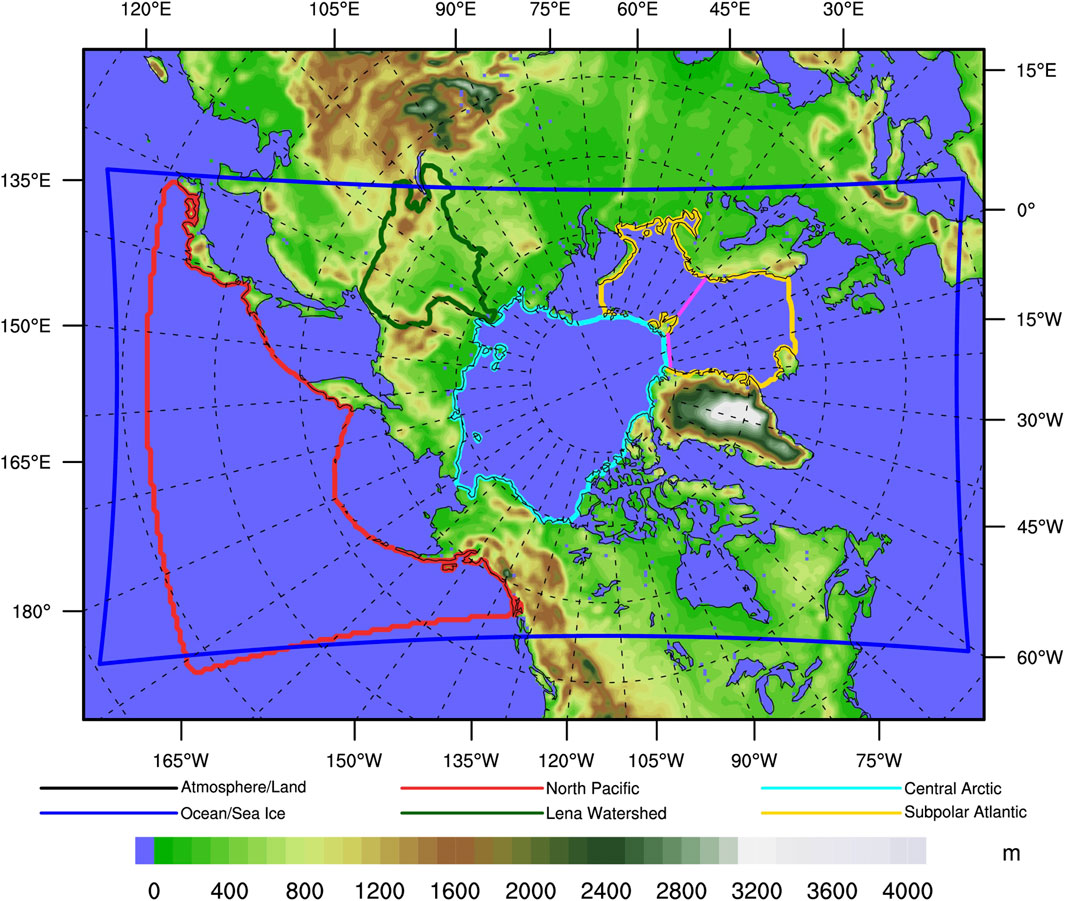
Figure 1. RASM model domains, topography, and analysis regions. The 50-km atmosphere/land domain covers the entire map region. The 9-km ocean/sea ice domain is indicated by the blue line. The North Pacific, Lena Watershed, Central Arctic, and Subpolar Atlantic analysis regions are outlined in red, dark green, cyan, and yellow. The color bar indicates the topography contours. The Fram Strait and Barents Sea Opening gateways for oceanic transport are indicated in magenta.
A modified version of the Advanced Research WRF (WRF-ARW, hereafter simply WRF, Skamarock et al., 2008) model v3.7.1 is used as the atmospheric component model in RASM. The modifications to WRF address the coupling processes, exchange of fluxes, and the progression of WRF through model time in concert with the other component models. The CPL7 coupler exchanges surface fluxes and state variables from the land, ocean, and sea ice component models every 20 min of model time. The initial and lateral boundary conditions for WRF in RASM are provided by the forcing dataset, such as a reanalysis or a global ESM. Additionally, grid nudging of temperature and wind (u and v) is applied to the top half of the model domain (above ∼540 hPa). The lateral boundary conditions and nudging values for WRF are updated from the forcing dataset in 6-h intervals.
Modifications are made to WRF physics parameterizations, including surface layer, microphysics, cumulus, and shortwave and longwave radiation parameterizations, to work in the fully coupled model framework and to improve results in the Arctic. The selected WRF physics parameterizations are based on extensive evaluations of different combinations of parameterizations that were shown to produce the best surface state in the fully coupled RASM. The RRTMG (Iacono et al., 2008) parameterizations are used for the shortwave and longwave radiation schemes. Modifications were made to the RRTMG parameterizations to export direct and diffuse visible and near-infrared solar radiation to CPL7 and to import direct and diffuse visible and near-infrared albedo. Such partitioning of the radiation and albedo is included for use in the physics of the coupled RASM model components. The selected microphysics parameterization is the Morrison scheme (Morrison et al., 2009) with modifications to pass the droplet size to the radiation parameterizations for the calculation of radiative fluxes. The Grell 3D scheme, with shallow convection, is used for the cumulus parameterization. A modification was made to the Grell 3D scheme so that the shallow convection is only applied to the grid points over the ocean. Sub-grid cloud fraction interaction is provided by the cumulus parameterization to the radiation schemes to account for the radiative impact of the convective clouds. The planetary boundary layer parameterization is handled by the Mellor-Yamada Nakanishi and Niino Level 2.5 scheme (MYNN 2.5; Nakanishi and Niino, 2006). The integrated land model in WRF is disabled in RASM. Instead, the surface fluxes, albedo and state values are provided by the VIC, POP, and CICE component models and exchanged through the CPL7 coupler. The Revised MM5 surface layer scheme (Jiménez et al., 2012) is the selected surface layer parameterization with extensive modifications to work with the exchange of fluxes from the coupler.
The list of variables (see Cassano et al., 2017; Table 2) exchanged between WRF and the coupler in RASM is nearly identical to those passed between the atmospheric model and the coupler in CESM. The fluxes and state variables exchanged between WRF with the coupler are time-averaged over the 20-min coupling time step. Area weighted sensible heat, latent heat, and momentum fluxes from VIC, CICE, and POP are passed to WRF for grid cells at land-ocean boundaries and/or with both sea ice and open ocean. The atmospheric surface stability is determined in CICE and CPL7 for the ice and ocean (Roberts et al., 2015) and VIC for the land (Hamman et al., 2016).
2.2 Decadal Prediction Large Ensemble
The CESM Decadal Prediction Large Ensemble (CESM-DPLE; Yeager et al., 2018) provides initial, lateral boundary, and nudging conditions for the atmospheric forcing with RASM. The DPLE provides an ensemble of initialized simulations that can be compared to the uninitialized 40-member ensemble of historical and projection (1920–2,100) simulations in the CESM Large Ensemble (CESM-LE; Kay et al., 2015). The DPLE was created with the same CESM code base, version 1.1, component model configurations, and radiative forcing as in the CESM-LE. There are 62 first of November start dates spanning 1954 to 2015, each with an integration of 122 months. The initial conditions for the atmosphere and land models were obtained from a single member of the CESM-LE. The ocean and sea ice initial conditions were from a coupled ocean-sea ice configuration of CESM v1.1 with historical atmospheric state and flux fields exchanged at the surface. Each DPLE start date has 40 ensemble members. The different ensemble members were generated by round-off perturbations applied to the atmospheric initial conditions. Only the initial 10 ensemble members archived the 6-hourly resolution atmospheric fields necessary for dynamical downscaling using RASM. WRF input files were created from the DPLE following that of Bruyère et al. (2015), including the WRF Preprocessing System (WPS v3.7.1) software, with modifications to some of the Bruyère et al. (2015) scripts to work with the DPLE data. The surface and sub-surface fields in the WRF input files were not necessary with RASM using a fully coupled modeling framework. Bias correction was not applied to the WRF input files from the DPLE data for reasons that will be covered in the discussion. The DPLE datasets were also regridded to the RASM atmosphere 50-km horizontal resolution domain to provide a direct comparison to the RASM simulations. These regridded datasets are hereinafter referred to as CESM-DPLE.
2.3 Reanalyses
Reanalysis datasets are used in the study to provide the initial and lateral boundary conditions, and nudging data for RASM simulations forced by reanalyses. The European Centre for Medium Range Weather Forecasts (ECMWF) Interim Re-Analysis (ERA-Interim, hereinafter referred to as ERAI; Dee et al., 2011) is the primary reanalysis used for this study. The Climate Forecast System Reanalysis (CFSR, hereinafter referred to as CFS; Saha et al., 2010b) from the National Centers for Environmental Prediction (NCEP) is used to provide a comparative reanalysis dataset and reanalysis forced RASM simulation. Lindsay et al. (2014) reviewed seven atmospheric reanalyses for the Arctic and concluded that ERAI and CFS were two of the three reanalyses that emerged as being the most consistent in comparison to observations of surface temperature, radiative fluxes, precipitation, and wind speed. The ERAI and CFS datasets were retrieved from the NCAR–Research Data Archive (NCAR-RDA; ERAI: European Centre for Medium-Range Weather Forecasts, 2009; CFS; Saha et al., 2010a). The ERAI and CFS datasets were also regridded to the RASM atmosphere 50-km horizontal resolution domain to provide a direct comparison to RASM simulations. The regridded datasets in the results sections are referred to as ERAI and CFS.
2.4 Experimental setup
Two fully coupled RASM simulations forced by reanalyses, ERAI (referred to hereafter as: RASM-ERAI) and CFS (referred to as: RASM-CFS) are completed for comparisons to the DPLE-forced RASM simulations. The three-dimensional initial state of the atmosphere is from the corresponding reanalysis state of the atmosphere for 00 UTC 1 September 1979. The sea ice and ocean initial states for the fully coupled reanalysis forced RASM simulations are from a RASM ocean-sea ice simulation starting from January 1958 to August 1979 with JRA-55 forcing and runoff (Kobayashi et al., 2015). The 1 September 1979 land surface initial state is from a 31-year uncoupled VIC simulation forced with meteorological inputs (Hamman et al., 2016). The RASM POP ocean temperature and salinity, along the closed lateral boundaries, are restored to monthly values from the Polar Science Center Hydrographic Climatology version 3.0 (PHC 3.0) (Steele et al., 2001), as described in Roberts et al. (2015). The RASM-ERAI and RASM-CFS simulations were initialized on 1 September 1979 and run through 31 December 2018 and 2020, respectively. Comparisons across the two reanalysis forced RASM simulations provides an understanding of the range of differences in RASM simulations when forced with approximately the same weather, as would be expected in two reanalyses.
The focus of the RASM simulations in this study is on the 10-member ensemble of RASM simulations forced by atmospheric output from the corresponding CESM-DPLE simulations with a start date of 1 December 1985. The RASM simulations were run for 121 months, through 31 December 1995 and are referred to as the RASM-DPLE ensemble. The results of this ensemble are compared to each other, a historical period to reanalyses (ERAI and CFS) spanning 1986 to 1995, RASM simulations forced by reanalyses (RASM-ERAI and RASM-CFS), and the source output from the CESM-DPLE ensemble simulations. The atmosphere in each RASM-DPLE simulation is initialized with the three-dimensional atmospheric state from the forcing data at the initial time. The land surface, ocean, and sea ice states are initialized from the RASM-ERAI simulation. The initialized values for each ensemble member match the start date of the ensemble member to that of the RASM-ERAI simulation. In other words, the 1 December 1985 RASM-DPLE ensemble start date uses the 00 UTC 1 December 1985 conditions from the RASM-ERAI simulation starting on 1 September 1979. Spatial two-dimensional plots of atmospheric state variables and regional plots of atmospheric state variables (not shown) were evaluated for the initial 30 days and there were no discontinuities or abrupt shifts indicated in the atmospheric analyses. This indicates that the initializations for the RASM-DPLE simulations present no need for an initial period of model spin up.
Two ensemble members from the RASM-DPLE ensemble were run a second time with a change to one of the WRF physics parameterization options. This modification to the WRF simulations was created to highlight the dependency of the RASM-DPLE results on the atmospheric model configuration in RASM. An additional ERAI forced RASM simulation was also run with the same WRF physics parameterization options. Past published (Cassano et al., 2017) and unpublished studies with WRF and RASM have revealed a modest change in the surface state variables and energy fluxes in the Arctic with a change in the cumulus parameterization. The alternate WRF physics configuration uses the Kain-Fritsch cumulus parameterization (Kain, 2004) instead of the G3. The Kain-Fritsch scheme includes the option for including the radiative impact of clouds but it does not include the built-in shallow convection scheme as applied over ocean points with the G3 cumulus parameterization. The modified RASM simulation forced with the ERAI reanalysis is hereinafter referred to as RASM_alt-ERAI. The RASM-DPLE simulations are initialized with the land, ocean, and sea ice from 1 December 1985 conditions of the RASM_alt-ERAI simulation. These RASM-DPLE simulations are hereinafter referred to as RASM_alt-DPLE_01 and RASM_alt-DPLE_02. All RASM simulations were completed using RASM tag 2_2_01. Table 1 provides a summary of the RASM simulations used in this study.
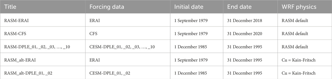
Table 1. List of RASM simulations with the simulation name, forcing data, initial date, end date, and specification of the WRF physics in RASM. RASM Simulations.
3 Results
3.1 Analysis of annual means of atmospheric state
Analyses of annual means of atmospheric state variables and fluxes reveals variability in the weather of RASM-DPLE simulations forced by the 10 CESM-DPLE ensemble members. The term weather is used in this study to denote the variation in atmospheric state as the result of the evolving patterns of the atmosphere that comprise the annual and multiyear monthly means. The annual and multiyear monthly means are not inherently weather, but it is differences in the variability and changes of weather patterns that results in differences in the respective means.
Figure 2 is a plot of annual means, from 1986 to 1995, of atmospheric state values (height and temperature for 300, 500, 700, and 850 hPa constant pressure surfaces, referenced as Z300, T300, Z500, T500, Z700, T700, Z850 and T850; sea level pressure and temperature at the surface, referenced as SLP and T_sfc) for the Central Arctic region (see Figure 1 for region boundaries). The left side of Figure 2 shows the results for the 10 RASM-DPLE simulations, 2 RASM reanalysis simulations, a RASM-DPLE ensemble mean, and the forcing data. The plots indicate the range and variability of the conditions for the 10 RASM-DPLE ensemble members for each year over the course of the 10-year simulation. RASM-DPLE_01 and RASM-DPLE_02 are plotted in red and green to highlight that these two ensemble members largely fall within the range of the overall 10 ensemble members used in this study. As is expected, these two ensemble members do, in some years, represent the upper and lower bounds of the 10 ensemble members, but overall they are not any more distinct than any of the other ensemble members.
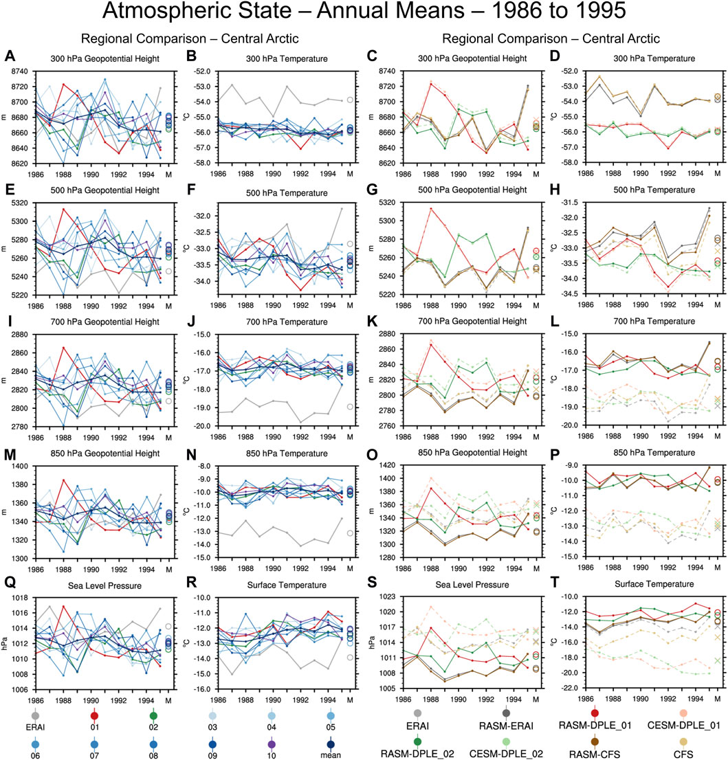
Figure 2. Annual means of atmospheric state for the Central Arctic analysis region spanning 1986 to 1995. The plotted values are of Z300 (A,C), T300 (B,D), Z500 (E,G), T500 (F,H), Z700 (I,K), T700 (J,L), Z850 (M,O), T850 (N,P), SLP (Q,S), and T_sfc (R,T). The left two columns are for the 10 RASM-DPLE ensemble member simulations (01—red, 02—green, 03 to 10 shades of blue), the RASM-DPLE ensemble mean (purple), and the ERAI reanalysis (light gray). The right two columns are of the RASM simulations (solid lines) and the forcing data (dashed lines) for reanalyses (ERAI - grays, CFS—browns) and DPLE (01—reds, 02—greens). The open circles (Xs) are the 10-year means for the RASM simulations (forcing data).
The right side of Figure 2 compares the two selected RASM-DPLE ensemble members (01 and 02) with the corresponding CESM-DPLE ensemble members, which are providing the atmospheric forcing data. The right side also includes the annual means from the RASM simulations forced by reanalyses (RASM-ERAI, RASM-CFS) and the corresponding values from the reanalyses (ERAI, CFS). Table 2 provides quantitative statistical measures (bias, correlation), for six of the atmospheric state fields in Figure 2, for 12 pairs of RASM simulations/forcing data. In Table 2, lines one to four compare RASM simulation to their respective forcing data, five to eight compare the RASM simulations with different forcing data, and 9–12 compare the forcing data. In Figure 2 it can be seen that at 500 hPa and 300 hPa the RASM simulations (solid lines) of geopotential height (Z500 and Z300) and temperature (T500, T300) closely follow the corresponding driving data (dashed lines of same general color) as is expected with nudging applied to the RASM/WRF simulations at heights approximately above 540 hPa. The distinct patterns of year-to-year changes in atmospheric state reflect the different weather in each dataset, the range of which is shown in the plot of the ten ensemble members. The results at 500 and 300 hPa indicate that individual RASM simulations follow closely the weather variability in the forcing data and that there is a range of weather conditions represented across the ten ensemble members. As mentioned previously, this reference to weather is not meant in the literal sense but instead it is used to indicate the variation in atmospheric patterns that when comprised together result in the differences in the plotted annual means in Figure 2 and calculated biases and correlations in Table 2. The RASM simulations, closely following the corresponding driving data, is represented in Table 2 by the large correlation values (approximately 1.00) between the RASM simulations and their respective forcing data (lines 1–4) for Z300 and T300. The differences between the DPLE ensemble members (RASM and CESM; reds and greens) and the reanalyses (RASM and reanalysis; browns and grays) shows that the ensemble members have different mean states (a bias) compared to the reanalyses. For example, the DPLE-based RASM simulations and forcing data (reds and greens) have a cold bias at 300 hPa and 500 hPa in comparison to the reanalyses-based RASM and forcing data (grays and browns). The T300 biases in lines 6–7, 11–12 of Table 2 are approximately −2.0 °C. This contrasts with approximately no bias between the RASM simulations and the corresponding forcing data (similar colors, solid lines in comparison to dashed lines). Table 2 shows T300 biases in lines one to four that are less than −0.1 °C. In the lower levels (700 hPa, 850 hPa, and surface), the RASM simulations continue to have distinct patterns of year-to-year variability corresponding to the DPLE and reanalyses forcing data. The correlations between the RASM simulations and the corresponding forcing data (lines 1–4 in Table 2) remain at or near 1.00 for Z850 and approximately 0.90 for T850. The slightly decreased correlations for T850 in the RASM simulations indicate the RASM physics and coupled surface states playing a role in the temperature patterns apart from the forcing data. Meanwhile, the bias patterns that were identified in the upper levels are reversed in the lower levels. At lower levels, the RASM simulations (darker colors, solid lines), whether forced by reanalyses or DPLE, have similar annual mean temperatures. Table 2 indicates T850 biases across the RASM simulations (lines 5–8) of less than 0.2°C, no matter the forcing data. Instead, there are warm biases in the RASM simulations (darker colors, solid lines) in comparison to that of the forcing data (lighter colors, dashed lines) for the Central Arctic. This is indicated in Table 2 with T850 biases between RASM simulations and their corresponding forcing data (lines 1–4) of approximately 2.9 °C. The cold bias in the upper levels, between the DPLE-based and reanalysis-based RASM simulations and forcing data, has been replaced with a warm bias between the RASM simulations and the forcing data. This suggests that the RASM model physics plays a dominant role in defining a new mean climatic state in the lower levels of the atmosphere. Meanwhile, the distinct interannual variability from the forcing data remains imprinted on the RASM simulations as is seen by the pattern of interannual variability (following the same weather) of the RASM simulations following that of the forcing data. This indicates that the RASM simulations develop a similar mean state, below the nudged upper portion of the model domain, but they also maintain the imprint of the weather variability (changes in annual means due to the cumulative differences in atmospheric patterns) in the driving data. The biases between DPLE versus reanalyses in the upper levels switches to biases between RASM simulations and forcing data in the lower levels. Similar results can be seen for the North Pacific and Lena regions (see Supplementary Figure S1; Supplementary Tables S1,S2).
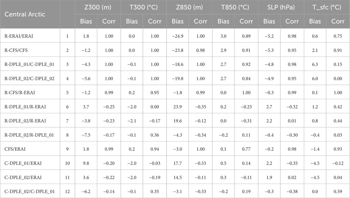
Table 2. Statistical measures of bias and correlation of the for a select number of pairings between RASM simulations and forcing data corresponding to the plots on the right-half of Figure 2. All values are for the Central Arctic region (see Figure 1). Lines one to four compare RASM simulation to their respective forcing data, five to eight compare across the RASM simulations with different forcing data, and 9–12 compare across the forcing data. The statistical measures are made for geopotential height at 300 and 850 hPa (Z300, Z850), temperature at 300 and 850 hPa (T300, T850), sea level pressure (SLP), and surface temperature (T_sfc). The units of bias for each field are included in the header line.
The atmospheric circulation of the RASM simulations and associated forcing data is evaluated with spaghetti plot analyses of a common single 500 hPa geopotential height contour (e.g., 5,400 m) plotted from each data source (Figure 3). The selected single height contour was based on an appropriate height to show the complete upper-level circulation pattern for the selected month or annual evaluation across the Arctic. The results show the variability and range of weather patterns for the 10 RASM-DPLE ensemble members for a given month (Figures 3A–F) and a given year (Figure 3G–L). For example, each ensemble member for January 1986 (Figure 3A) has a 500 hPa ridge over the west coast of North America but the amplitude and position of that ridge is different for each ensemble member. The variability in the weather across the RASM-DPLE simulations remains in the annual means, although not as pronounced as in the monthly means. RASM-DPLE_01 and RASM-DPLE_02 are highlighted (red, green) and the two ensemble members are representative of the range of conditions across the ensemble (Figures 3A–C,G–I), similar to what was indicated in the regional atmospheric state analyses for the ensemble (Figure 2). Spaghetti plots comparing the RASM simulations (darker colors) to the forcing data (lighter colors) (Figures 3D–F, J–L) indicate that the weather at 500 hPa in the RASM simulations matches that of the forcing data with only small differences. This is as is expected for a dynamical downscaling simulation that is nudged to the forcing data for the top half of the model.
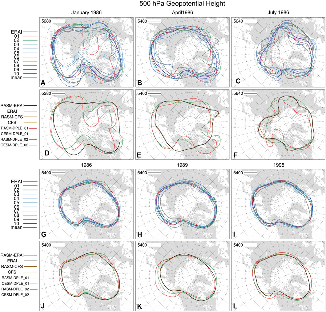
Figure 3. Spaghetti plot of a single 500 hPa geopotential height contour for the RASM domain. The top two rows are monthly means for January (A,D), April (B,E), and July (C,F) 1986 and the bottom two rows are annual means for 1986 (G,J), 1989 (H,K), 1995 (I,L). The contour is 5,400 m for all panels except January 1986 (A,D): 5,280 m) and July 1986 (C,F): 5,640 m). The first (A-C) and third (G-I) rows are for the 10 RASM-DPLE ensemble member simulations (01—red, 02—green, 03 to 10 shades of blue), the RASM-DPLE ensemble mean (purple), and the ERAI reanalysis (light gray). The second (D-F) and fourth rows (J-L) are of the RASM simulations (darker colors) and the forcing data (lighter colors) for reanalyses (ERAI - grays, CFS - browns) and DPLE (01—reds, 02—greens).
3.2 Regional analyses including alternate RASM simulations
Additional RASM simulations (RASM_alt-ERAI, RASM_alt-DPLE_01, and RASM_alt-DPLE_02) with alternate WRF physics configuration are included in the following results to highlight the role of the model’s atmospheric physics. The only difference in the WRF configuration is the selection of the cumulus parameterization (see Sect. 2.4 for more details). Figure 4 is a plot of the atmospheric state for the annual cycle of monthly means across the 10 years (1986–1995) for the RASM simulations (solid lines for RASM_std and darker colors, short-dashed lines for RASM_alt) and the forcing data (lighter colors, long-dashed lines) for the Central Arctic region) (Supplementary Figure S2 is the same plot but for the North Pacific and Lena regions.). The plotted values are referred to as anomalies and are calculated as the multiyear monthly mean for the data source minus the ERAI multiyear monthly mean. The plotting of ERAI reference anomalies is used to remove the large annual cycle and allows for the variability across the selected simulations to be more easily seen and it is not done in making a reference to the ERAI values as being the “truth”. The pattern of the Central Arctic annual cycle of geopotential heights and temperature at 500 hPa and 300 hPa for the RASM simulations follows closely to that of the corresponding forcing data (similar colors) with little sensitivity to the RASM atmospheric physics configuration. The DPLE means indicate a cold bias, relative to ERAI, of approximately 2 °C at 300 hPa and 0.5 °C for the Central Arctic region. The imprint of the weather at 300 hPa and 500 hPa is evident from the similar patterns of variability in the RASM simulations and the forcing data (similar colors), although the pattern of the annual cycle for the RASM simulations has some deviations from that of the forcing data in temperature at 500 hPa. This deviation is indicating the influence of the lower levels on the upper levels.
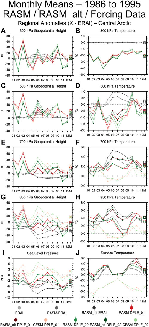
Figure 4. 10-year (1986–1995) monthly means indicating the annual cycle of the atmospheric state for the Central Arctic analysis region. The plotted values are of Z300 (A), T300 (B), Z500 (C), T500 (D), Z700 (E), T700 (F), Z850 hPa (G), T850 hPa (H), SLP (I), and T_sfc (J). The plotted means are for the RASM_std simulations (solid lines), RASM_alt simulations (short-dashes, darker colors) and the forcing data (long dashes, lighter colors) for the ERAI reanalysis (grays) and DPLE (01—reds, 02—greens). The open circles, open squares, and Xs are the 10-year means for the RASM_std, RASM_alt simulations, and forcing data. The means are plotted as anomalies in comparison to the ERAI reanalysis.
At lower levels (700 hPa and below), the annual cycle of temperature displays three clusters–RASM simulations (solid lines), RASM_alt simulations (short-dashed lines) and the CESM-DPLE forcing data (long-dashed lines). The difference between the ERAI and CESM-DPLE forcing data indicates a cold bias, relative to ERAI, in surface temperature (Tsfc) for the CESM-DPLE simulations. This cold bias of Tsfc in the DPLE forcing data is completely absent in the RASM simulations, with even the annual cycle of Tsfc bias in the DPLE forcing and RASM-DPLE simulations showing different patterns. The North Pacific region (Supplementary Figure S2) shows the most pronounced impact on the Tsfc due to the changes in the RASM physics with clear distinctions between RASM simulations (solid lines), RASM_alt simulations (short-dashed lines) and the CESM-DPLE forcing data (long-dashed lines). Past studies (Jousse et al., 2015; Cassano et al., 2017) have found the low-level stratocumulus clouds of this region are particularly sensitive to the selection of WRF physics options. This demonstrates that the atmospheric physics of the different RASM configurations dominates the 10-year mean surface climate state. Similar comments on the patterns and biases can be made regarding the temperature at 850 hPa and 700 hPa levels. At these levels the biases from the DPLE forcing is combined with the impact of the RASM model physics in determining the annual cycle in the 10-year climate. While there is an offset (bias) in geopotential height between the RASM simulations and forcing data the pattern of the 10-year annual cycle of the RASM simulations for geopotential height in the lower half of the model follows the same general pattern as the forcing data. This indicates that the differences in the weather patterns from the forcing data is still imprinted on the RASM simulations in the lower levels of the atmosphere. The Central Arctic region has slightly different levels of clustering across the RASM_std and RASM_alt simulations and the forcing data depending on the impact of the change in the RASM configuration for the Central Arctic region and time of year.
Analyses of the fluxes at the surface emphasize the dependence of the model physics on the results for the lower atmosphere. Figure 5 is a plot of monthly means of surface fluxes and precipitation for the 10-year RASM_std and RASM_alt simulations and the corresponding forcing data for the Central Arctic (Supplementary Figure S3 is the same plot but for the North Pacific and Lena regions.). The shortwave downwelling radiation (SWD; Figure 5A) indicates three groups of results with the individual CESM-DPLE, RASM_std, and RASM_alt simulations clustered together by simulation type (similar line style). The CESM-DPLE simulations have the most SWD, the RASM_std simulations the least, and the RASM_alt simulations in between the two. The longwave downwelling radiation (LWD; Figure 5B) also indicates the results clustered by simulation type and mostly independent of the forcing data, with the differences in biases between RASM_alt and RASM_std changing slightly over the course of the annual cycle. The sum of sensible heat and latent heat (SH + LH; Figure 5C) shows similar clustering by simulation type but with the larger differences in biases between RASM_std and RASM_alt during the second half of the annual cycle. Precipitation in the Central Arctic (Figure 5D) does not display as clear a separation between the RASM, RASM_alt and DPLE simulations as the radiative and turbulent fluxes but distinct clusters for precipitation are more obvious in the North Pacific (Supplementary Figure S3D) and Lena (Supplementary Figure S3H). The results in analyzing the surface fluxes and precipitation indicate that the model physics plays the largest role in the climate of the surface energy fluxes and atmospheric state in the lower atmosphere. A change in the WRF physics parameterizations (e.g., planetary boundary layer, microphysics, and cumulus parameterizations) will produce a different mean climatic state no matter the forcing data.

Figure 5. Same as Figure 4 except means of surface fluxes (SWD (A), LWD (B), SH+LH (C)) and total precipitation (D).
3.3 Spatial analyses of atmospheric state and surface fluxes
Analyses of spatial patterns of Z500, LWD, and Tsfc, with annual and seasonal (December-January-February, DJF; June-July-August, JJA) means for 1986, provide additional understanding of the similarities and differences in the RASM simulations and forcing data. The differences of Z500 (Figure 6), between RASM simulations and forcing data, provides a greater understanding of the relative dependencies with the dynamical downscaling using RASM. There are minimal differences in Z500 between the RASM simulation and forcing data (ERAI, Figure 6A; DPLE_01; Figure 6C). These results are similar to what was indicated previously with the regional plots of atmospheric state (Figures 2, 4) and the Z500 spagehtti plot (Figure 3). This is also true for the RASM_alt simulation with changes in WRF physics (RASM_alt-ERAI–RASM-ERAI, Figure 6B). This indicates that the atmospheric circulation for the top half of the RASM model is constrained by the nudging to the forcing data, as is expected. Meanwhile, the differences in the weather between the DPLE_01 and ERAI forcing data (CESM-DPLE_01—ERAI, Figure 6E) are reflected with similar patterns of differences between RASM simulations dependent on forcing data (RASM-DPLE_01—RASM-ERAI, Figure 6D) and in comparing the RASM-DPLE_01 simulation to ERAI (RASM-DPLE_01—ERAI, Figure 6F). The differences in Z500 represent the changes in the atmospheric circulation for the top half of the RASM simulations between DPLE_01 and ERAI. The results for the temperature at 500 hPa (Supplementary Figure S3) show similar results with minimal differences indicated between the RASM simulation and its forcing data and larger differences when comparing results between DPLE_01 and ERAI, in either the RASM simulation and/or the forcing data.
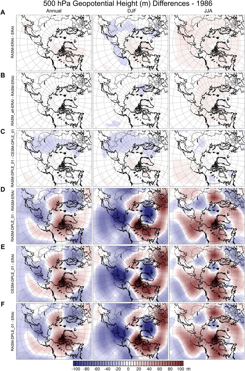
Figure 6. Spatial plots of differences in 500 hPa geopotential height (Z500) for 1986 across the RASM domain. The means are annual, December-January-February, and June-July-August in the columns from left to right. The differences are between RASM simulations/forcing data and other RASM simulations/forcing data as labeled along the left side of each row [(A): RASM-ERAI - ERAI, (B): RASM_alt-ERAI - RASM-ERAI, (C): RASM-DPLE_01 - CESM-DPLE_01, (D): RASM-DPLE_01 - RASM-ERAI, (E): CESM-DPLE_01 - ERAI, (F): RASM-DPLE_01 - ERAI]. The color bar indicates the contour of differences in mean Z500 with blues (negative) and reds (positive) differences.
The spatial differences in LWD across the RASM simulations and forcing data (Figure 7) highlight the predominant dependence of RASM and the model physics on the results for LWD. The differences in LWD in RASM-ERAI and ERAI (Figure 7A) indicate that RASM has more LWD compared to ERAI over almost the entire RASM domain. This is an inherent RASM bias in relation to ERAI. Similar differences in LWD are found in the comparison between the RASM-DPLE_01 and ERAI (Figure 7F) highlighting the dominance of the inherent RASM biases over the differences in weather for 1986 between DPLE_01 and ERAI. A comparison of RASM with the alternate WRF physics and the RASM standard configuration (Figure 7B) indicates that the change in WRF physics results in a decrease in LWD across the entire ocean regions of the RASM domain for the annual mean and the winter mean. The results also indicate a decrease in LWD over land downwind of the ocean regions. There is less difference for the summer months of 1986 over the RASM region, except for the lower-latitude ocean. Meanwhile the results for LWD radiation between RASM simulations with different forcing data (Figure 7D) indicate relatively small differences, in comparison to that of differences in the modeling systems (Figures 7A–C), across the RASM domain for the annual and seasonal means, except for the Central Arctic in the winter. These results highlight that the model physics plays a larger role on the annual and seasonal means than the differences in weather for 1986 but the difference in weather still has a small imprint. A comparison of LWD in CESM-DPLE_01 and ERAI (Figure 7E) indicates that CESM has seasonally varying differences in LWD in relation to ERAI. These differences are similar for CESM-DPLE_01 (Figure 7D) and CESM-DPLE_02 (not shown) indicating that these are inherent differences in CESM relative to ERAI, are most dependent on the differences in model physics (CESM vs. ERAI) and less so due to the differences in the weather. A similar analysis of SWD (Supplementary Figure S4) shows results indicating that the SWD is largely a function of the model physics (CESM/RASM vs. ERAI and RASM_alt vs. RASM) with some regional sensitivity to the driving data (ERAI versus DPLE_01). These results for LWD (Figure 7) and SWD (Supplementary Figure S4) are opposite of that for the Z500 (Figure 6) indicating the larger role that the model biases, and model physics, have on the downwelling radiation at the surface, in comparison to changes in the weather of the simulations (forcing data).
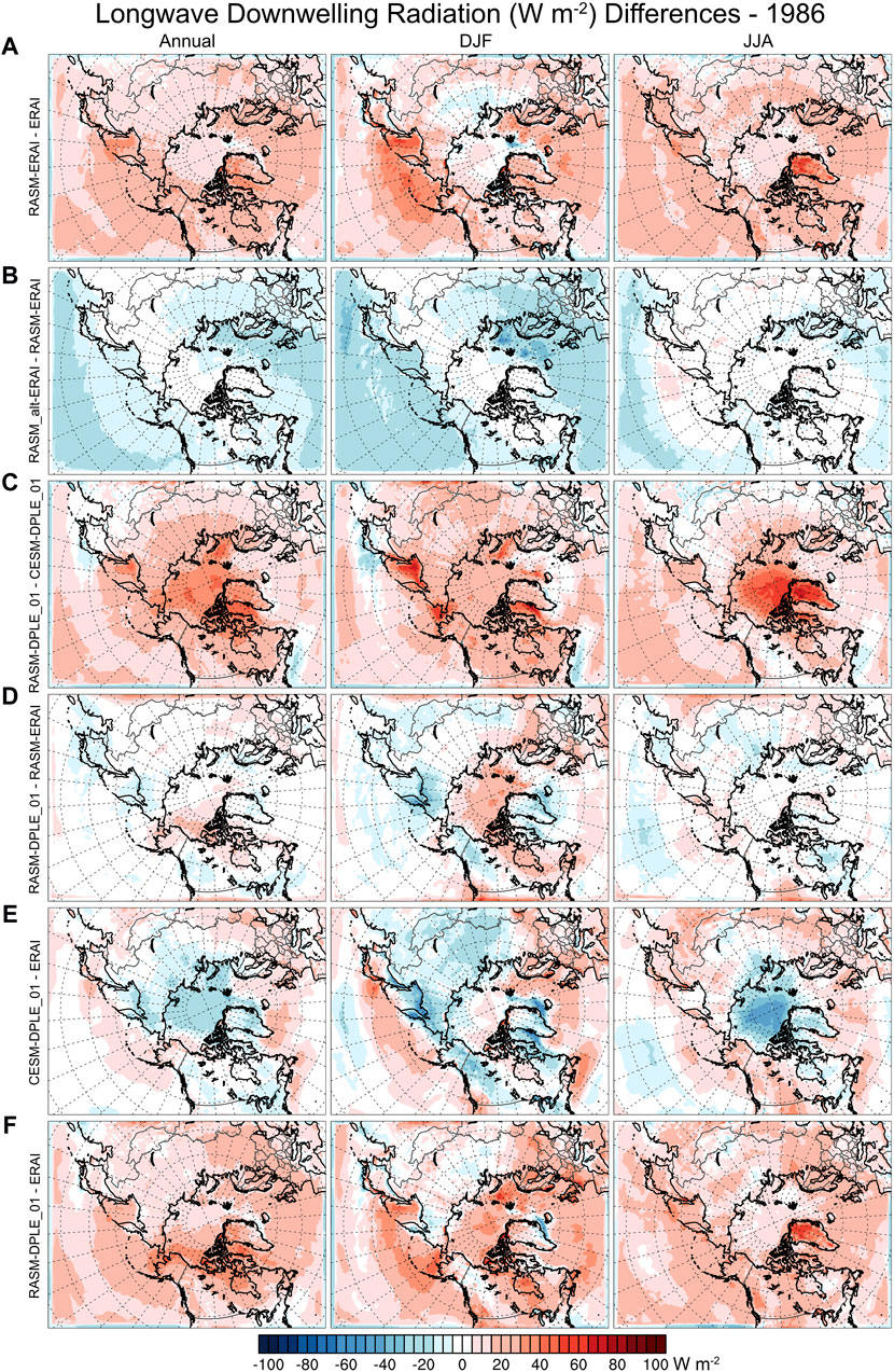
Figure 7. Same as Figure 6 except means of longwave downwelling radiation at the surface (LWD). The color bar indicates the contour of differences in mean LWD with blues (negative) and reds (positive) differences.
Comparisons of spatial differences of Tsfc across the different RASM simulations and forcing data for 1986 (Figure 8) show varying dependencies related to changes in the forcing data (weather), model and changes in modeling system/physics. The differences in Tsfc between RASM-ERAI and ERAI (Figure 8A) indicate that RASM has a warm bias over most land areas and a slight cold bias over the sub-polar oceans (year-round) and a cold bias over the central Arctic (DJF). These differences reflect RASM’s preferred climate state, or inherent model biases in comparison to ERAI. At least a part of the positive Tsfc biases are likely associated with the positive differences in LWD at the surface (Figure 8A). The comparison of CESM-DPLE_01 and ERAI (Figure 8E) shows that CESM-DPLE_01 has a cold bias relative to ERAI in most areas (annually and DJF) but some regional warm biases in the summer. The differences in this comparison reflect both the inherent biases in CESM Tsfc relative to ERAI and the differences in seasonal and annual weather for this ensemble member compared to the weather in ERAI for 1986. These cold biases for CESM in relation to ERAI were previously indicated in the regional plots for the RASM domain and the Central Arctic (Figures 2D,H). The Tsfc in RASM-DPLE_01 relative to RASM-ERAI (Figure 8D) reflects the unique weather of this ensemble member in relation to ERAI for the specific seasons and year for 1986. A comparison of differences in Tsfc between RASM simulations with the modified WRF physics and that of the standard RASM configuration (Figure 8B) shows a slight warm difference across the North Pacific, western Siberia, eastern Canada, and the north Atlantic for the annual mean. RASM_alt-ERAI has a slight cool difference relative to RASM-ERAI over the land areas for the DJF mean. Meanwhile for JJA there are moderate warm differences across the entire RASM domain, except the Central Arctic. The Tsfc differences between RASM_alt and RASM_std (Figure 8B) are slightly smaller in magnitude than the differences between RASM-ERAI and ERAI (Figure 8A) indicating that even a single change in the model physics can significantly alter the Tsfc. In summary, the results for Tsfc across the RASM simulations and forcing data for 1986 (Figure 8) indicate a reverse of that of Z500 (Figure 6) with changes in model system (Figures 6A,C, 8A,C) and changes in model configuration (panels: B) presenting larger differences than the changes in weather (DPLE ensemble members or ERAI, panels: D).
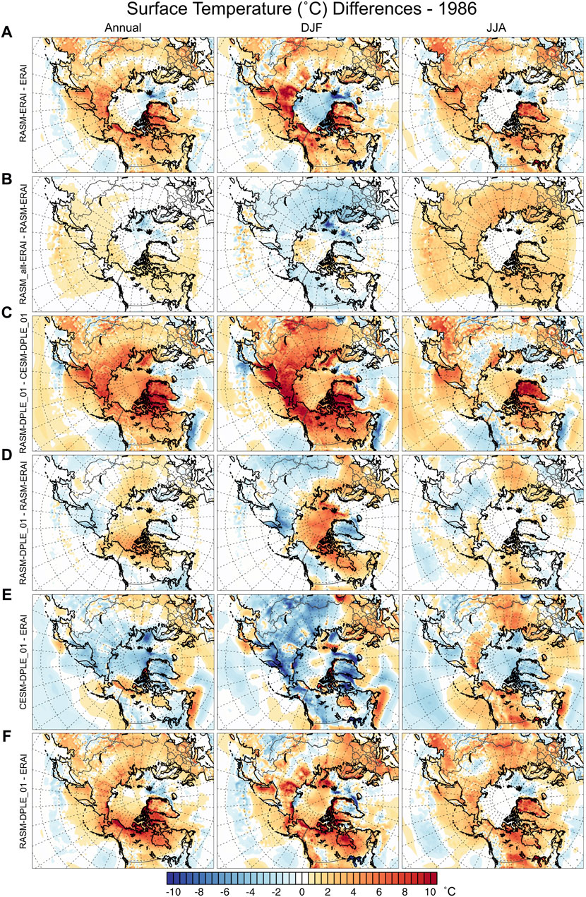
Figure 8. Same as Figure 6 except means of surface temperature (Tsfc). The color bar indicates the contour of differences in mean Tsfc with blues (negative) and oranges/reds (positive) differences.
3.4 Evaluation of sea ice and ocean transport in the RASM-DPLE ensemble
The analyses presented above demonstrate that the dynamical downscaling of the CESM-DPLE ensemble members by RASM results in the top half of the model following that of the forcing data as a result of using nudging in RASM. In contrast, the near surface state and radiative fluxes are clustered more closely among modeling systems (CESM, RASM, and reanalyses), and model configuration (RASM_std vs. RASM_alt) than due to the differences in the weather (forcing data: reanalyses and DPLE ensemble members). Despite the strong control the modeling system and model configuration have on near surface state and radiative fluxes there is still a signal from differences in weather across the different forcing data. As a result the fully-coupled RASM simulations display differences in sea ice and oceanic transport that varies with forcing data.
Figure 9 is a spatial plot showing sea ice extent for the RASM simulations and NSIDC sea ice observations for March 1995 (Figures 9A,C) and September 1995 (Figures 9B,D), representing the results 10 years into the RASM-DPLE simulations. The top two panels (Figures 9A,B) show all 10 RASM-DPLE ensemble members and the ensemble mean. The Chukchi, East Siberian, and Laptev seas in particular shows large variations in the sea ice extent for September 1995 (Figure 9B) depending on the variability and changes of weather patterns in a given DPLE ensemble member. The impact of the changes in WRF physics in RASM (RASM_alt) simulations going to a different surface climate state are indicated in the lower panels (Figures 9C,D) with the dashed lines indicating the modified WRF physics. For March 1995 (Figure 9C) the RASM_alt simulations for the same ensemble member have a slightly larger sea ice extent than the corresponding RASM_std simulations for the same ensemble member (similar color). The sea ice extent for the RASM_alt simulations is less than that of the RASM_std simulations for September 1995 (Figure 9D). This is reflective of the warmer Tsfc conditions during JJA in the RASM_alt simulations than the RASM simulations as previously indicated in Figure 8B over the western Arctic. Figure 10 is a time series plot of sea ice volume from the RASM simulations and PIOMAS (Zhang and Rothrock, 2003; Schweiger et al., 2011) reference values from 1986 to 1995. The time series plot of all 10 RASM-DPLE ensemble members shows that despite RASM model producing a similar near-surface climate state for the 10 years across the ensemble members, the variability and changes of weather patterns results in different sea ice results across the RASM-DPLE ensemble members. A review of the differences in RASM simulations with and without modified WRF physics (Figure 10B) shows that in general the modified WRF physics output is resulting in less sea ice in the fully coupled RASM simulations. Hence, the modification in the WRF physics accounts for a change in the fully coupled sea ice conditions. It can also be seen that the decadal trend between the RASM_std and RASM_alt simulations for each ensemble member are similar.
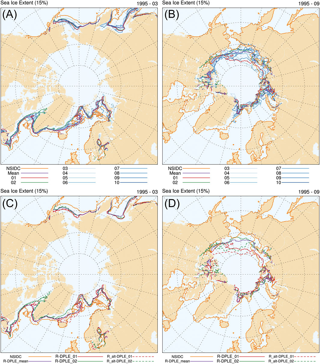
Figure 9. Spaghetti plot of sea ice extent, defined as 15% sea ice concentration, for March 1995 (A,C) and September 1995 (B,D) from the RASM simulations and the observations from the National Snow and Ice Data Center (NSIDC) as a reference. The top row (A,B) is of the 10 RASM-DPLE ensemble member simulations (01—red, 02—green, 03 to 10 shades of blue), the RASM-DPLE ensemble mean (purple), and NSIDC (orange). The bottom row (C,D) is of the RASM_std-DPLE 01 and 02 simulations (solid lines), RASM_alt-DPLE 01 and 02 simulations (dashed lines), the RASM_std-DPLE ensemble mean (purple) and the NSIDC observations (orange).
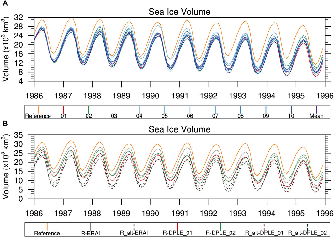
Figure 10. Time series plot of sea ice volume spanning 1986 to 1995. The top row (A) is of the 10 RASM-DPLE ensemble member simulations (01—red, 02—green, 03 to 10 shades of blue), the RASM-DPLE ensemble mean (purple), and PIOMAS reference (orange). The bottom row (B) is of RASM_std simulations (ERAI, 01, 02; solid lines), RASM_alt simulations (ERAI, 01, 02; dashed lines, darker colors), and PIOMAS reference (orange).
The impacts of the different DPLE ensemble members on the RASM fully coupled climate system extend to that of oceanic volume transport. Figure 11 shows the net volume transport across two main gateways between the North Atlantic and the Arctic Ocean: the Barents Sea Opening (Figures 11A,C) and Fram Strait (Figures 11B,D). At times a given ensemble member will have the largest amount of volume transport for a given month and at times that same ensemble member will have the least. The comparison of the RASM_std and RASM_alt simulations (Figures 11C,D) show comparable variability with the RASM_std simulations (solid lines) representing higher volume transport across the Barents Sea Opening compared to that from the RASM_alt simulations (dashed lines).
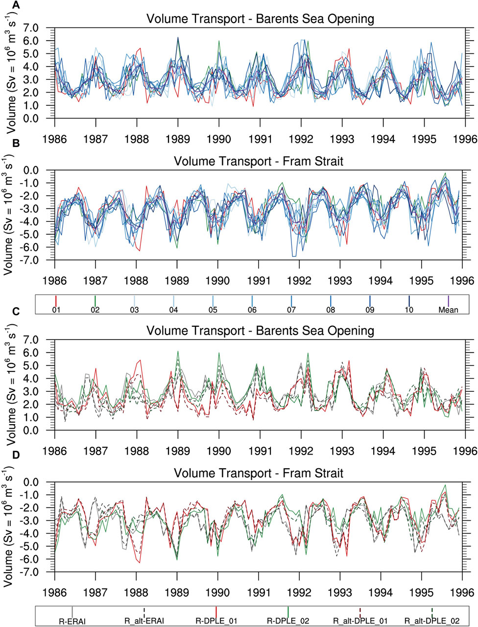
Figure 11. Time series plot of oceanic volume transport through the Barents Sea Opening (A,C) and the Fram Strait (B,D) gateways. The top two rows (A,B) are of the 10 RASM-DPLE ensemble member simulations (01—red, 02—green, 03 to 10 shades of blue) and the RASM-DPLE ensemble mean (purple). The bottom two rows (C,D) are of RASM_std simulations (ERAI, 01, 02; solid lines) and the RASM_alt simulations (ERAI, 01, 02; dashed lines, darker colors).
4 Discussion
This study has evaluated the results of the dynamical downscaling of ESM and reanalysis data by the fully coupled RASM. This version of RASM has atmosphere, land, ocean, and sea ice component models that exchange fluxes and state values through a coupler. After the initialization, the land, ocean, and sea ice models evolve freely based on their interactions with the atmosphere and the respective model evolution. This contrasts with the more frequently used dynamical downscaling with an atmosphere-only model that has prescribed lower boundary conditions from either the forcing ESM or a secondary dataset, such as satellite observations of sea surface temperature. The ability for RASM to evolve at the surface more freely, without prescribed lower-boundary conditions, highlights one of the unique aspects of this study.
An ensemble of RASM simulations was created using 10 members of the CESM-DPLE, two reanalyses, and two versions of RASM that differ in their model physics. This ensemble of RASM simulations allows for the evaluation of the relative role of differences in weather, differences due to biases in the driving data, and differences due to changes in the modeling system. The first 10 ensemble members of the CESM-DPLE project, with a start date of 1 November 1985, are used to provide the ESM forcing data for the dynamical downscaling in RASM. An advantage to using 10 ensemble members from the CESM-DPLE is that it allows for an evaluation of differences due solely to changes in the of the weather across the 10 ensemble members. The term weather in this context is used to denote the temporal variation in atmospheric state as the result of the evolving atmospheric patterns that produce the annual and multiyear monthly means. Two RASM simulations were completed using the ERAI and CFS reanalyses running from September 1979 through 2018 (2020 for CFS). Comparison of the reanalysis forced RASM simulations with the DPLE forced simulations allows for an assessment of the impact of biases in the driving data (CESM-DPLE) on the downscaled climate state. An alternate RASM configuration (RASM_alt) was configured with a change in the selected cumulus parameterization in the WRF model. The RASM_alt configuration is used to highlight the dependency of the results on the configuration of the atmospheric model in RASM.
The analyses presented in this study are from the 10 RASM-DPLE ensemble members, two reanalyses, and RASM_alt simulations. Two ensemble members (DPLE 01 and 02) were selected for a more careful examination with a comparison to the reanalyses and the corresponding CESM-DPLE forcing data. The RASM simulations of the two ensemble members and the two reanalyses indicate that for the 300 hPa and 500 hPa geopotential height and temperature fields the mean climatic state matches that of the corresponding forcing data (either reanalysis or CESM-DPLE). This is the expected result for dynamical downscaling simulations where nudging to the forcing data is applied to the top half of the model. The position and amplitude of ridges and troughs of geopotential height at 500 hPa for any given month or year also indicate a strong correlation between the RASM simulations and the forcing data (Figure 3).
The results of the mean climatic state, as indicated in the annual and multiyear means, for the lower half of the model domain for the atmosphere tend to form three clusters: i) RASM simulations with either CESM or reanalysis forcing data, ii) CESM-DPLE, and iii) reanalyses. RASM and CESM both have biases relative to the reanalyses, but RASM-DPLE simulation biases are unique from the biases in the CESM-DPLE forcing data used for these simulations and are similar to the RASM-ERAI biases. For example, annual means of Tsfc for the 10-year simulations across the RASM domain show the RASM simulations (DPLE and reanalysis) with a warm bias in relation to ERAI and the CESM-DPLE forcing data as a cold bias in relation to ERAI (Figure 2T). The biases that are present in the CESM-DPLE forcing data are no longer present in the RASM-DPLE simulations.
The mean climatic state of the lower part of the RASM atmosphere is largely independent of the nudging to the forcing data and is instead dependent on RASM’s inherent biases, atmospheric physics parameterizations, and presumably resolution, in driving the near surface state in the model. The RASM_alt simulations result in a different mean state of the lower atmosphere and surface as indicated by Tsfc and the surface fluxes (Figure 5) because of the change of a single physics parameterization (the cumulus parameterization). The changes in the forcing data (across DPLE ensemble members or in comparison to the reanalyses) are not large enough to change the clouds and fluxes that form the mean RASM climatic state for the lower atmosphere and surface.
The results indicate that despite the mean surface climatic state being similar across the ensemble of 10-year RASM-DPLE simulations there are differences in how the model reaches that mean climatic state. Those differences are in the variability and changes of weather patterns, or the sequence and intensity of the atmospheric circulation, over the 10 years that produce the mean climatic state. These differences in weather are indicated in the year-to-year patterns in annual means (Figure 2), and the differences in the position and amplitude of the ridges and troughs in the 500 hPa geopotential spaghetti plots (Figure 3). The RASM-DPLE simulations produce weather that is unique for each ensemble member, and that is consistent with the CESM-DPLE driving data as indicated by similar year-to-year patterns in the analyses (Figure 2). The differences in the variability and changes of weather patterns across the 10 ensemble members results in variances in the sea ice state (Figures 9, 10), and the oceanic transport into and out of the Arctic (Figure 11). This is similar to how there are differences in sea ice and oceanic states from year-to-year in recent history despite the minimal differences in the year-to-year mean climatic state.
Bias correction to ESM data is a common prerequisite in using ESM output for forcing of RCMs. In this study it was found that the bias correction of the ESM data was not necessary in the fully coupled modeling framework. There is a level of independence between the upper half of the model domain, where nudging is applied to the forcing data, and what happens at the surface in that the biases in the DPLE temperature have no, or insignificant, impact on the results for the lowest part of the atmosphere. Instead, it is the physics parameterizations of the atmospheric model that play the dominant role in establishing the mean climatic state of the lower atmosphere and near surface conditions. The results indicate that it is possible to do downscaling with a biased ESM and obtain reasonable and improved results at the surface. The key difference as to why this is the case for this study, in contrast to previous studies with an atmosphere-only RCM framework, is that the surface conditions are not prescribed by the ESM forcing data but evolve freely through coupling between the atmosphere and the other component models.
The benefits of a fully coupled RESM lie in the ability of the model to respond to the larger scale weather, accomplished through the nudging to the ESM or reanalysis forcing data, meanwhile the higher spatial and temporal resolution, in combination with the more region-specific and flexible atmospheric physics in the RESM, allows the lower portion of the atmosphere and the coupled model components to freely evolve, largely independent of the forcing data. Changes or improvements to a RESM atmospheric physics impact the mean climatic state of the atmospheric and coupled components of the RESM. In the case of RASM, the Arctic-optimized configuration of the ocean model, and the higher spatial and temporal resolutions of the ocean and sea ice models, allow for a more realistic representation of the physical processes and mechanisms for the Arctic climate system.
Data availability statement
The datasets presented in this study can be found in online repositories. The names of the repository/repositories and accession number(s) can be found below: https://www.cesm.ucar.edu/community-projects/dple.
Author contributions
MS: Conceptualization, Data curation, Formal Analysis, Funding acquisition, Investigation, Methodology, Project administration, Resources, Software, Validation, Writing–original draft, Writing–review and editing. JC: Conceptualization, Formal Analysis, Funding acquisition, Investigation, Methodology, Project administration, Resources, Supervision, Validation, Writing–original draft, Writing–review and editing. YL: Data curation, Formal Analysis, Validation, Visualization, Writing–review and editing. WM: Conceptualization, Funding acquisition, Project administration, Resources, Validation, Writing–review and editing. AC: Data curation, Methodology, Software, Writing–review and editing. RO: Data curation, Software, Validation, Writing–review and editing.
Funding
The author(s) declare that financial support was received for the research, authorship, and/or publication of this article. This research was supported by the Regional and Global Model Analysis (RGMA) component of the Earth and Environmental System Modeling (EESM) program of the United States Department of Energy’s Office of Science, as a contribution to the HiLAT-RASM project. Computing resources for the RASM simulations were provided by the United States Department of Defense (U.S. DoD) High Performance Computer Modernization Program (HPCMP). The CESM-DPLE ensemble was generated using computational resources provided by the National Energy Research Scientific Computing Center (NERSC), which is supported by the Office of Science of the United States.
Conflict of interest
The authors declare that the research was conducted in the absence of any commercial or financial relationships that could be construed as a potential conflict of interest.
Publisher’s note
All claims expressed in this article are solely those of the authors and do not necessarily represent those of their affiliated organizations, or those of the publisher, the editors and the reviewers. Any product that may be evaluated in this article, or claim that may be made by its manufacturer, is not guaranteed or endorsed by the publisher.
Supplementary material
The Supplementary Material for this article can be found online at: https://www.frontiersin.org/articles/10.3389/feart.2024.1392031/full#supplementary-material
References
Bowden, J. H., Otte, T. L., Nolte, C. G., and Otte, M. J. (2012). Examining interior grid nudging techniques using two-way nesting in the WRF model for regional climate modeling. J. Clim. 25, 2805–2823. doi:10.1175/jcli-d-11-00167.1
Bruyère, C. L., Done, J. M., Holland, G. J., and Fredrick, S. (2013). Bias corrections of global models for regional climate simulations of high-impact weather. Clim. Dyn. 43, 1847–1856. doi:10.1007/s00382-013-2011-6
Bruyère, C. L., Monaghan, A. J., Steinhoff, D. F., and Yates, D. (2015). Bias-corrected CMIP5 CESM data in WRF/MPAS intermediate file format. Boulder, CO: National Center for Atmospheric Research.
Bullock, O. R. J., Alapaty, K., Herwehe, J. A., Mallard, M. S., Otte, T. L., Gilliam, R. C., et al. (2014). An observation-based investigation of nudging in WRF for downscaling surface climate information to 12-km grid spacing. J. Appl. Meteorology Climatol. 53, 20–33. doi:10.1175/jamc-d-13-030.1
Cassano, J. J., DuVivier, A., Roberts, A., Hughes, M., Seefeldt, M., Brunke, M., et al. (2017). Development of the Regional Arctic System Model (RASM): near-surface atmospheric climate sensitivity. J. Clim. JCLI-D-15-0775.1 30, 5729–5753. doi:10.1175/jcli-d-15-0775.1
Cassano, J. J., Higgins, M. E., and Seefeldt, M. W. (2011). Performance of the Weather Research and Forecasting model for month-long pan-arctic simulations. Mon. Weather Rev. 139, 3469–3488. doi:10.1175/mwr-d-10-05065.1
Craig, A. P., Vertenstein, M., and Jacob, R. (2012). A new flexible coupler for earth system modeling developed for CCSM4 and CESM1. Int. J. High. Perform. Comput. Appl. 26, 31–42. doi:10.1177/1094342011428141
Dee, D. P., Uppala, S. M., Simmons, A. J., Berrisford, P., Poli, P., Kobayashi, S., et al. (2011). The ERA-Interim reanalysis: configuration and performance of the data assimilation system. Q. J. R. Meteorological Soc. 137, 553–597. doi:10.1002/qj.828
European Centre for Medium-Range Weather Forecasts: ERA-Interim Project (2009). Research Data Archive at the National Center for Atmospheric Research, Computational and Information Systems Laboratory. doi:10.5065/D6CR5RD9
Giorgi, F. (2019). Thirty years of regional climate modeling: where are we and where are we going next? J. Geophys. Res. Atmos. 124, 5696–5723. doi:10.1029/2018jd030094
Giorgi, F., and Gao, X.-J. (2018). Regional earth system modeling: review and future directions. Atmos. Ocean. Sci. Lett. 11, 189–197. doi:10.1080/16742834.2018.1452520
Glisan, J. M., Gutowski, W. J. J., Cassano, J. J., and Higgins, M. E. (2013). Effects of spectral nudging in WRF on arctic temperature and precipitation simulations. J. Clim. 26, 3985–3999. doi:10.1175/jcli-d-12-00318.1
Gutowski, W. J., Ullrich, P. A., Hall, A., Leung, L. R., O’Brien, T. A., Patricola, C. M., et al. (2020). The ongoing need for high-resolution regional climate models: process understanding and stakeholder information. Bull. Am. Meteorological Soc. 101, E664–E683. doi:10.1175/bams-d-19-0113.1
Hamman, J., Nijssen, B., Brunke, M., Cassano, J., Craig, A., DuVivier, A., et al. (2016). Land surface climate in the regional arctic system model. J. Clim. 29, 6543–6562. doi:10.1175/jcli-d-15-0415.1
Hamman, J., Nijssen, B., Roberts, A., Craig, A., Maslowski, W., and Osinski, R. (2017). The coastal streamflow flux in the regional arctic system model. J. Geophys Res. Oceans 122, 1683–1701. doi:10.1002/2016jc012323
Hoffmann, P., Katzfey, J. J., McGregor, J. L., and Thatcher, M. (2016). Bias and variance correction of sea surface temperatures used for dynamical downscaling. J. Geophys Res. Atmos. 121 (12), 877–890. doi:10.1002/2016jd025383
Hunke, E., Allard, R., Bailey, D. A., Blain, P., Craig, A., Damsgaard, A., et al. (2018). CICE-Consortium/CICE: CICE version 6.0.0 (CICE6.0.0). Available at: https://zenodo.org/records/1893041.
Hurrell, J. W., Holland, M. M., Gent, P. R., Ghan, S., Kay, J. E., Kushner, P. J., et al. (2013). The community earth system model: a framework for collaborative research. Bull. Am. Meteorological Soc. 94, 1339–1360. doi:10.1175/bams-d-12-00121.1
Iacono, M. J., Delamere, J. S., Mlawer, E. J., Shephard, M. W., Clough, S. A., and Collins, W. D. (2008). Radiative forcing by long-lived greenhouse gases: calculations with the AER radiative transfer models. J. Geophys Res. Atmos. 1984 2012 113. doi:10.1029/2008jd009944
Jiménez, P. A., Dudhia, J., González-Rouco, J. F., Navarro, J., Montávez, J. P., and García-Bustamante, E. (2012). A revised scheme for the WRF surface layer formulation. Mon. Weather Rev. 140, 898–918. doi:10.1175/mwr-d-11-00056.1
Jousse, A., Hall, A., Sun, F., and Teixeira, J. (2015). Causes of WRF surface energy fluxes biases in a stratocumulus region. Clim. Dyn. 46, 571–584. doi:10.1007/s00382-015-2599-9
Kain, J. S. (2004). The Kain–Fritsch convective parameterization: an update. J. Appl. Meteorol. 43, 170–181. doi:10.1175/1520-0450(2004)043<0170:tkcpau>2.0.co;2
Kay, J. E., Deser, C., Phillips, A., Mai, A., Hannay, C., Strand, G., et al. (2015). The Community Earth System Model (CESM) Large Ensemble project: a community resource for studying climate change in the presence of internal climate variability. Bull. Am. Meteorological Soc. 96, 1333–1349. doi:10.1175/bams-d-13-00255.1
Kinney, J. C., Maslowski, W., Osinski, R., Jin, M., Frants, M., Jeffery, N., et al. (2020). Hidden production: on the importance of pelagic phytoplankton blooms beneath Arctic sea ice. J. Geophys Res. Oceans 125. doi:10.1029/2020jc016211
Kobayashi, S., Ota, Y., Harada, Y., Ebita, A., Moriya, M., Onoda, H., et al. (2015). The JRA-55 reanalysis: general specifications and basic characteristics. J. Meteor. Soc. Jpn. 93, 5–48. doi:10.2151/jmsj.2015-001
Liang, X., Lettenmaier, D. P., Wood, E. F., and Burges, S. J. (1994). A simple hydrologically based model of land surface water and energy fluxes for general circulation models. J. Geophys Res. Atmos. 99, 14415–14428. doi:10.1029/94jd00483
Liang, X., Wood, E. F., and Lettenmaier, D. P. (1996). Surface soil moisture parameterization of the VIC-2L model: evaluation and modification. Glob. Planet Change 13, 195–206. doi:10.1016/0921-8181(95)00046-1
Lindsay, R., Wensnahan, M., Schweiger, A., and Zhang, J. (2014). Evaluation of seven different atmospheric reanalysis products in the Arctic. J. Clim. 27, 2588–2606. doi:10.1175/jcli-d-13-00014.1
Liu, P., Tsimpidi, A. P., Hu, Y., Stone, B., Russell, A. G., and Nenes, A. (2012). Differences between downscaling with spectral and grid nudging using WRF. Atmos. Chem. Phys. 12, 3601–3610. doi:10.5194/acp-12-3601-2012
Maslowski, W., Kinney, J. C., Higgins, M., and Roberts, A. (2012). The future of arctic Sea Ice. Annu. Rev. Earth Pl. S. C. 40, 625–654. doi:10.1146/annurev-earth-042711-105345
Morrison, H., Thompson, G., and Tatarskii, V. (2009). Impact of cloud microphysics on the development of trailing stratiform precipitation in a simulated squall line: comparison of one- and two-moment schemes. Mon. Weather Rev. 137, 991–1007. doi:10.1175/2008mwr2556.1
Nakanishi, M., and Niino, H. (2006). An improved Mellor–Yamada Level-3 Model: its numerical stability and application to a regional prediction of advection fog. Bound-lay Meteorol. 119, 397–407. doi:10.1007/s10546-005-9030-8
Powers, J. G., Klemp, J. B., Skamarock, W. C., Davis, C. A., Dudhia, J., Gill, D. O., et al. (2017). The weather research and forecasting model: overview, system efforts, and future directions. Bull. Am. Meteorological Soc. 98, 1717–1737. doi:10.1175/bams-d-15-00308.1
Roberts, A., Craig, A., Maslowski, W., Osinski, R., DuVivier, A., Hughes, M., et al. (2015). Simulating transient ice–ocean ekman transport in the Regional Arctic System Model and Community Earth System Model. Ann. Glaciol. 56, 211–228. doi:10.3189/2015aog69a760
Saha, S., Moorthi, S., Pan, H., Wu, X., Wang, J., Nadiga, S., et al. (2010a). NCEP climate Forecast system reanalysis (CFSR) 6-hourly products, January 1979 to December 2010. Research Data Archive at the National Center for Atmospheric Research, Computational and Information Systems Laboratory. doi:10.5065/D69K487J
Saha, S., Moorthi, S., Pan, H.-L., Wu, X., Wang, J., Nadiga, S., et al. (2010b). The NCEP Climate Forecast System Reanalysis. Bull. Am. Meteorological Soc. 91, 1015–1058. doi:10.1175/2010bams3001.1
Schweiger, A., Lindsay, R., Zhang, J., Steele, M., Stern, H., and Kwok, R. (2011). Uncertainty in modeled Arctic sea ice volume. J. Geophys Res. 116, C00D06. doi:10.1029/2011jc007084
Sitz, L. E., Sante, F. D., Farneti, R., Fuentes-Franco, R., Coppola, E., Mariotti, L., et al. (2017). Description and evaluation of the Earth System Regional Climate Model (Reg CM-ES). J. Adv. Model Earth Sy 9, 1863–1886. doi:10.1002/2017ms000933
Skamarock, W. C., Klemp, J. B., Dudhia, J., Gill, D. O., Barker, D., Duda, M. G., et al. (2008). A description of the Advanced Research WRF version 3. Boulder, Colorado, United States: University Corporation for Atmospheric Research.
Smith, R., Jones, P., Bryan, F., Danabasoglu, G., Dennis, J., Dukowicz, J., et al. (2010). The Parallel Ocean Program (POP) reference manual ocean component of the Community Climate System Model (CCSM) and Community Earth System Model (CESM). Los Alamos, NM: Los Alamos National Laboratory. Available at: https://www.cesm.ucar.edu/models/cesm2/ocean/doc/sci/POPRefManual.pdf.
Steele, M., Morley, R., and Ermold, W. (2001). PHC: a global ocean hydrography with a high-quality Arctic Ocean. J. Clim. 14, 2079–2087. doi:10.1175/1520-0442(2001)014<2079:pagohw>2.0.co;2
White, R. H., and Toumi, R. (2013). The limitations of bias correcting regional climate model inputs. Geophys Res. Lett. 40, 2907–2912. doi:10.1002/grl.50612
Xu, Z., Han, Y., Tam, C.-Y., Yang, Z.-L., and Fu, C. (2021). Bias-corrected CMIP6 global dataset for dynamical downscaling of the historical and future climate (1979–2100). Sci. Data 8, 293. doi:10.1038/s41597-021-01079-3
Xu, Z., and Yang, Z.-L. (2015). A new dynamical downscaling approach with GCM bias corrections and spectral nudging. J. Geophys. Res. Atmos. 120, 3063–3084. doi:10.1002/2014jd022958
Yeager, S. G., Danabasoglu, G., Rosenbloom, N., Strand, W., Bates, S., Meehl, G., et al. (2018). Predicting near-term changes in the Earth System: a large ensemble of initialized decadal prediction simulations using the Community Earth System Model. Bull. Am. Meteorological Soc. 99, 1867–1886. doi:10.1175/bams-d-17-0098.1
Yu, X., Rinke, A., Dorn, W., Spreen, G., Lüpkes, C., Sumata, H., et al. (2020). Evaluation of Arctic sea ice drift and its dependency on near-surface wind and sea ice conditions in the coupled regional climate model HIRHAM–NAOSIM. Cryosphere 14, 1727–1746. doi:10.5194/tc-14-1727-2020
Zhang, J., and Rothrock, D. A. (2003). Modeling global sea ice with a thickness and enthalpy distribution model in generalized curvilinear coordinates. Mon. Weather Rev. 131, 845–861. doi:10.1175/1520-0493(2003)131<0845:mgsiwa>2.0.co;2
Keywords: dynamical downscaling, regional earth system model, fully coupled, nudging, Arctic, atmospheric state, sea ice
Citation: Seefeldt MW, Cassano JJ, Lee YJ, Maslowski W, Craig AP and Osinski R (2024) Evaluation of dynamical downscaling in a fully coupled regional earth system model. Front. Earth Sci. 12:1392031. doi: 10.3389/feart.2024.1392031
Received: 26 February 2024; Accepted: 20 May 2024;
Published: 19 June 2024.
Edited by:
Lin Wang, Chinese Academy of Sciences (CAS), ChinaReviewed by:
Thomas Ballinger, University of Alaska Fairbanks, United StatesJianping Tang, Nanjing University, China
Copyright © 2024 Seefeldt, Cassano, Lee, Maslowski, Craig and Osinski. This is an open-access article distributed under the terms of the Creative Commons Attribution License (CC BY). The use, distribution or reproduction in other forums is permitted, provided the original author(s) and the copyright owner(s) are credited and that the original publication in this journal is cited, in accordance with accepted academic practice. No use, distribution or reproduction is permitted which does not comply with these terms.
*Correspondence: Mark W. Seefeldt, bWFyay5zZWVmZWxkdEBjb2xvcmFkby5lZHU=