Dynamic evolution of amplitude and position of geomagnetic secular acceleration pulses since 2000

Recent studies on the behavior of geomagnetic secular acceleration (SA) pulses have provided a basis for understanding the dynamic processes in the Earth’s core. This analysis statistically evaluates the evolution of the SA pulse amplitude and position since 2000 by computing the three-year difference in SA with the CHAOS-7 geomagnetic field model (CHAOS-7.17 release). Furthermore, the study explores the correlation between the acceleration pulse amplitude and geomagnetic jerks and the dynamic processes of alternating variation and polarity reversal of pulse patches over time. Research findings indicate that the variation in pulse amplitude at the Core Mantle Boundary (CMB) closely resembles that observed at the Earth’s surface, with an average period of 3.2 years. The timing of peak pulse amplitude aligns with that of the geomagnetic jerk, suggesting its potential utility as a novel indicator for detecting geomagnetic jerk events. The acceleration pulses are the strongest near the equator (2°N) and more robust in the high-latitude region (68°S) of the Southern Hemisphere, indicating that the variation is more dramatic in the Southern Hemisphere. The acceleration pulses fluctuate unevenly in the west-east direction, with characteristics of local variation. In the Western Hemisphere, the pulse patches are distributed near the equator, exhibiting an evident westward drifting mode. The positive and negative patches alternate in time, displaying a polarity reversal in the west-east direction, with an average interval of approximately 32°. These characteristics can be attributed to the rapid magnetic field fluctuations disclosed by the model of stratification at the top of the Earth’s core. In the Eastern Hemisphere, the pulses are weaker between 10°E and 60°E, with the most active pulses occurring around 80°E to 105°E and near 150°E. The pulse patches exhibit a broader distribution in the north-south direction, with relatively strong patches still occurring near 40°N and 40°S. These local variation characteristics match the actual cases of zonal flows and geostrophic Alfvén waves in the Earth’s core.

1 Introduction

The Earth’s main magnetic field and secular variations (SV) of the field are generated by the movement of the conductive fluid inside the Earth’s outer core. SV variations over shorter intervals of up to ten years can be detected by the field’s secular acceleration (SA) (Soloviev et al., 2017; Amit et al., 2018). Several recent studies have determined the geomagnetic SA pulses on sub-decadal time scales occurring at the CMB (Finlay et al., 2016; Lesur et al., 2018; Kloss and Finlay, 2019). These changes are related to the rapid flows at the Earth’s core surface (Mandea et al., 2010; Aubert and Finlay, 2019; Nahayo and Korte, 2022).

Geomagnetic jerks are an observed characteristic of rapid geomagnetic variations generated inside the Earth’s outer core (Holme et al., 2011; Pinheiro et al., 2011; Kotzé and Korte, 2016). In respect to the morphology, a geomagnetic jerk has a typical V shape or inverted V shape change, which is presented as an abrupt turn of the first derivative of the field ($\partial B/\partial t$); in the second derivatives of time series ($\partial B^2/\partial t^2$), jerks are shown as step-like, and sudden changes of SA polarity occurring in about a year at the junction of two time-intervals with linear SV changes (Mandea et al., 2010; Soloviev et al., 2017). The impulse of Dirac is seen in the third derivative ($\partial B^3/\partial t^3$) of the series, which marks the discontinuity of the step function (in this case, the SA). Here we defined SA pulse as extreme SA values. In recent years, satellite magnetic survey studies have shown that the geomagnetic acceleration forms pulse patches with different intensities at the CMB, and positive and negative polarities of SA patches exhibit alternating variation with a quasi-period of 6 years (Chulliat and Maus, 2014; Soloviev et al., 2017). The geomagnetic jerk typically occurs between two continuous SA pulses (Chulliat et al., 2010; Stefan et al., 2017; Aubert and Finlay, 2019). It has been confirmed that the rapid variations in geomagnetic SA are closely related to geomagnetic jerks (Olsen and Mandea, 2007; Chulliat et al., 2010; Chulliat and Maus, 2014; Ou et al., 2016). The secular acceleration pulses generated inside the outer core manifest as geomagnetic jerks observed in geomagnetic observation records (Xu, 2009; Mandea et al., 2010; Brown and Mound, 2013; Alken et al., 2020). Therefore, studying the geomagnetic acceleration of the Earth’s core is to study geophysical phenomena from the perspective of the Earth’s core dynamics, and studying the theory of its morphology and origin is an essential window to understanding the Earth’s core dynamics (Barrois et al., 2017; Metman et al., 2020; Aubert et al., 2022; Lesur et al., 2022).

In the Section 2, we calculate the geomagnetic SA based on the CHAOS-7 geomagnetic field model (Finlay et al., 2020) and use the three-year difference in acceleration to express the variation of acceleration pulses. In the Section 3, we statistically analyze the evolution of the amplitude and geographic position of acceleration pulses since 2000, examine the relationship between the amplitude of acceleration pulses and the geomagnetic jerks, and explore the possibility of predicting the occurrence of geomagnetic jerk events in the future and the identification method. Moreover, in the Section 4, we study the time variation of the position of acceleration pulses over time and the characteristic of spatial position reversal of positive and negative polarities. We also discuss the similarities and differences of acceleration pulses in the west-east and north-south directions. Finally, based on the above analyses, in the Section 5, we disclose the dynamic process of the spatiotemporal evolution of acceleration pulses, providing new bases and clues for profoundly understanding the Earth’s core dynamic process of geomagnetic acceleration pulses.

2 Data and methods

The CHAOS series geomagnetic field models were constructed initially by Olsen et al. (2006, 2009, 2014), and Finlay et al. (2016, 2020) updated and developed them. The models of this series were constructed with the magnetic field observation data obtained by near-Earth orbit satellites (e.g., Swarm, CryoSat-2, CHAMP, SAC-C, and Oersted) and the annual difference data of monthly average values observed at global ground stations. This model series has been developed for the seventh generation (CHAOS-7). The most remarkable feature is that the model coefficients can be updated in time according to the latest satellite and ground magnetic survey data. The latest CHAOS-7.17 is an expanded model of CHAOS-7. It uses the baseline data of Swarm L1b version 0602 up to 31st December 2023 and ground observatory data containing the available data up to the end of October 2023.

Using the CHAOS-7.17 model, we calculate the SV and SA of components X, Y, and Z at the Earth’s surface with the annual differential method. We truncate the model at degree and order 13. Since only the magnetic field radial component Br (Br = −Z) is continuous through the CMB, we analyze only the acceleration of the radial component of the magnetic field at the CMB. To focus on the large scale of the field, we also analyze the field truncated at degree and order 6 at the CMB (Chulliat and Maus, 2014; Aubert and Finlay, 2019; Campuzano et al., 2021).

The variation of the secular acceleration pulses (ΔSA) of each geomagnetic component is calculated to locate rapid variations in geomagnetic acceleration. This is done by differencing the time-averaged SA, using the method proposed by Olsen and Mandea (2007). The calculation formula (Eq. 1) is as follows:

$\Delta SA-B=\Delta \ddot{B}\left(t\right)={\ddot{B}}_{t+\Delta t}-{\ddot{B}}_{t-\Delta t}(1)$

B denotes geomagnetic elements, $\ddot{B}$ _t±Δt denotes the SA time series of B before and after Δt years of time point t. Where Δt = 0.5 year is the annual difference, normalized to 1 year. Δt = 1.0 year is 2-year difference, and Δt = 1.5 years are 3-year differences. Finally, we take Δt = 1.5 years. ΔSA-B is the three-year variation of SA. We have calculated the global distribution of geomagnetic components (ΔSA-X, ΔSA-Y, and ΔSA-Br) at the Earth’s surface and ΔSA-Br at the CMB at an interval of 0.1 years since 2000.

Figure 1 is the distribution diagram for the year 2021.0. It can be seen from Figure 1 that, in the low- and medium-latitude regions near the equator, the acceleration pulses of each geomagnetic component form multiple positive and negative patches, which, however, are distributed unevenly. At the Earth’s surface, there are positive and negative patches of ΔSA-X occurring on the south and north sides of the patches of radial component ΔSA-Br and positive and negative patches of ΔSA-Y occurring on the east and west sides of the patches of the component. There is a similar feature for other years. Such distribution morphology indicates that the positions of acceleration pulse patches vary with the geomagnetic component, and the phenomena caused by geomagnetic jerks also vary with the geomagnetic component. Comparison between Figures 1C, D shows that the positions of the positive and negative patches of ΔSA-Br at the Earth’s surface correspond to those at the CMB. However, due to such causes as magnetic field attenuation and different truncations (Nmax = 6 at the CMB and Nmax = 13 for the surface calculation), the distribution morphology of ΔSA-Br at the Earth’s surface differs from that of ΔSA-Br at the CMB. The number of patches at the CMB is more than that at the Earth’s surface, indicating that some acceleration pulses with small amplitude have largely attenuated before propagating to the Earth’s surface.

Figure 1

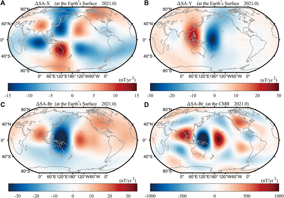
Figure 1. Global distribution of (A) ΔSA-X, (B) ΔSA-Y, and (C) ΔSA-Br at the Earth’s surface, and global distribution of (D) ΔSA-Br at the CMB for the year 2021.0.

To show the variations in amplitude and position of acceleration pulses, we identify the focal values and geographic positions of the maximum positive and negative patches of acceleration pulses for each year. We define the average of the maxima of positive patches(ΔSA_+MAX) and the absolute value of the maxima of negative patches(⎥ΔSA_-MAX⎥) of a geomagnetic component ΔSA as the amplitude of acceleration pulses, denoted as ΔSAA (Eq. 2),

$\Delta SAA=\left(\Delta S{A}_{+\mathit{MAX}}+\left|\Delta S{A}_{-\mathit{MAX}}\right|\right)/2(2)$

Figures 2A, B show the ΔSAA time series of the components X, Y, and Br at the Earth’s surface and the component Br at the CMB since 2000. Therefore, this paper mainly studies the variations in amplitude and geographic position of the patches with maxima of acceleration pulses.

Figure 2

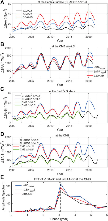
Figure 2. Variations of acceleration pulse amplitude with different Δt. (A) 3-year difference of the ΔSA-X, ΔSA-Y, and ΔSA-Br for the CHAOS7 model at the Earth’s surface; (B) 3-year difference of the maximum of SA (ΔSA_+MAX) and absolute values of the negative maximum of SA (|ΔSA_-MAX|), and ΔSAA-Br for the CHAOS7 model at the CMB; 1-year and 3-year difference of SA-Br for CHAOS7 and CM6 models (C) at the Earth’s surface; (D) at the CMB; (E) Amplitude spectrum in function of the period (frequency) of ΔSA-Br and ΔSAA-Br at the CMB.

We use the CHAOS7 model but change the Δt used to calculate the secular acceleration increment. We take the 1-year difference of the secular acceleration to statistically produce a time series of acceleration pulse amplitude (ΔSAA). The results show that the patterns of change using the 1-year and 3-year differences are the same, as shown inFigures 2C, D. At the CMB (Figure 2D), the extreme values of ΔSAA for the Br component of the 1-year difference and the 3-year difference (See Supplementary Table S1 for details) occur with the same frequency, and the time at which the maximum value occurs is nearly identical, with an average error of only 0.15 years; at the Earth’s surface (Figure 2C), the maximum values of ΔSAA for the Br component occur with the same frequency, and the average error of the time of occurrence of the extremes is 0.3 years. It proves that the cyclical patterns are the same, derived from the 1-year or 3-year difference. Different truncations can be the issue since small scales have much smaller timescales. The 1-year differential time series exhibits certain fluctuations, particularly at the Earth’s surface. However, the 3-year difference of ΔSAA exhibits a better average effect, with a smoother curve for extreme values than its 1-year counterpart. Therefore, in the following analysis, we discuss the temporal evolution of the acceleration pulse in terms of the 3-year difference.

Using the same method, we calculated the ΔSAA of the 1-year difference and 3-year difference of the Br component SA at the Earth’s surface and the CMB for the CM6 model (Sabaka et al., 2020). The results show that the time-series variations of the ΔSAA of the CM6 and CHAOS models are the same, as shown in Figures 2C, D. The results of the two models are similar, suggesting a 3-year variation in the ΔSAA time series. While the CM6 model spans a period of 1999.0∼2019.5, the CHAOS model covers a more extended period (the CHAOS-7.17 model spans 1997.1∼2024.1). Thus, we mainly focus on the results of the CHAOS-7.17 model.

3 Results

3.1 Variation in the amplitude of acceleration pulses

As can be discerned from Figure 2A, the maximum and minimum of the amplitude series of acceleration pulses do not occur simultaneously for three components, X, Y, and Br, at the Earth’s surface. However, they have identical trends of fluctuation over time. In the identification of a geomagnetic jerk, the SA of the component Y is typically used to express the feature of the jerk since the component Y is less sensitive to the variation of interference from external field sources (especially the magnetosphere) (Pavón-Carrasco et al., 2021). However, the component ΔSAA-Br of pulse amplitude is the highest, followed by the component ΔSAA-Y, and the component ΔSAA-X is the lowest. Consequently, we primarily investigate the characteristic of variation in ΔSAA-Br. Figure 2B shows the time series of absolute values of maxima of positive and negative patches of components ΔSA-Br and ΔSAA-Br at the CMB.

Figure 2 clearly shows that the amplitude of acceleration pulses of each geomagnetic component exhibits a prominent characteristic of periodic fluctuation. With the series of ΔSAA-Br at the CMB as an example, the maxima occurred in the years 2002.6, 2004.8, 2007.5, 2011.0, 2014.3, 2017.3, and 2020.3, respectively, and the minima happened in the years 2000.4, 2003.8, 2005.9, 2009.3, 2012.6, 2016.0, and 2019.1, respectively. The maximum interval between the two maxima is 3.5 years (from 2007.5 to 2011.0), and the minimum is 2.2 years (from 2002.6 to 2004.8). The average period is about 3.2 years, with uneven fluctuation periods. To determine the period of a series of SA pulses, we applied a Fast Fourier transform of ΔSA-Br and ΔSAA-Br at the CMB, as shown in Figure 2E. Periods corresponding to the maxima are about 3.1 years for a 3-year difference. Periods of other components are also 3.1 years for a 3-year difference and 3.2 years for a 1-year difference (Table 1). The most striking is that the occurrence time of maxima matches the occurrence time of geomagnetic jerk events, which has been reported since 2000 (Brown and Mound, 2013; Kotzé, 2017; Pavón-Carrasco et al., 2021). This fully indicates that the amplitude of acceleration pulses can graphically describe its variation and reflect the occurrence time of geomagnetic jerks.

Table 1

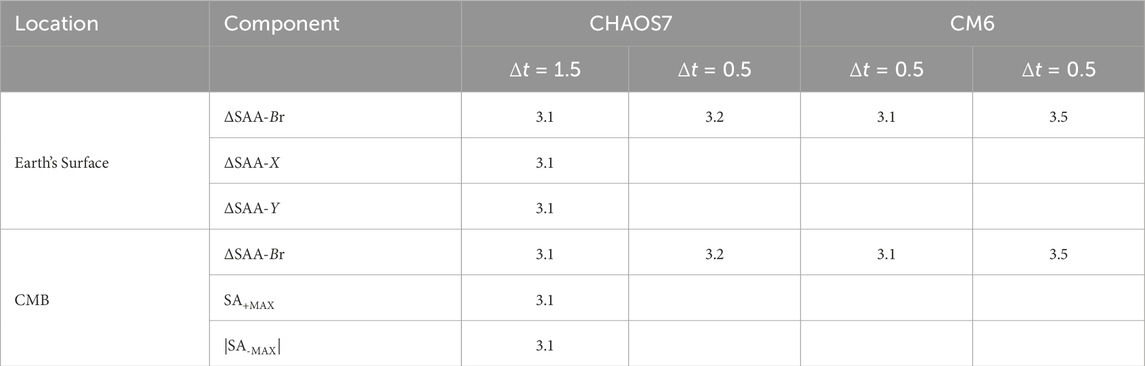
Table 1. Period of SA pulses (year).

3.2 Variation of the position of acceleration pulses

The position distribution, time-longitude diagram, and time-latitude diagram of the pulse patches can show the geographic positions of acceleration pulse patches and their evolution. Figure 3A shows the geographic positions of focal values of positive and negative patches of the component ΔSA-Br at the CMB since 2000 (at an interval of 0.5 years). It can be seen from Figure 3A that the position distribution characteristic of the maxima of patches is as follows: the maxima are mainly concentrated near the equator with a north-south span from 14°S to 18°N in the region from ∼10°E west to 150°W, and no maxima are occurring in the area from ∼10°E to 60°E. In the region from ∼60°E to 150°E, the maxima are relatively far from the equator with a north-south span from 35°S to 45°N. In the regions near 40°W and 0°, namely, the Atlantic Ocean and Western Africa, belts of dense maxima formed in the north-south direction. The distribution of geographic positions of the maxima of patches is uneven, suggesting that geomagnetic acceleration pulses have a regional feature.

Figure 3

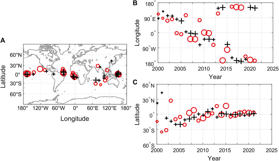
Figure 3. (A) Positions of the maximum values of positive and negative patches of ΔSA-Br at the CMB in 2000∼2021(on Miller’s cylindrical projection). (B) Changes in longitude of positive and negative maximum values with time, and (C) Changes in latitude of positive and negative maximum values with time. The black marker “+” represents the position of the positive maximum values and the red “○” denotes the position of the negative maximum values. Sizes of the markers represent the value of maximum and minimum ΔSA-Br.

Figures 3B, C show the longitude and latitude variations of the position of patches over time, respectively. It can be discerned from the figures that the variation of the position of the maxima of positive and negative patches since 2000 can be divided into three phases: 1) During the period from ∼2000 to 2006, the positions of patches were distributed from 80°E to 130°E in the Eastern Hemisphere (Figure 3A), with a larger span in the latitude direction from 35°S to 45°N (Figure 3B). 2) from ∼2006 to 2012.5, the positions of patches were distributed near the equator from 10°E to 80°W and moved from south to north over time. The belts of dense maxima near 40°W and 0° shown in Figure 3A occurred in this period. 3) Since 2012.5, the positions of patches have been distributed in the regions of the Pacific Ocean near the equator at 150°E and from 80°W to 160°W.

3.3 Variations of acceleration pulses in longitude and latitude directions

The time-longitude and time-latitude diagrams can even more clearly show the variation of the position of acceleration pulses. Figure 4A shows the time-longitude diagram of ΔSA-Br at the equator plane of the CMB. It can be seen from the figure that the main characteristic of the distribution of patches is alternating positive and negative polarities over time. The occurrence time of the patch polarities corresponds to the occurrence time of the maxima and minima of the amplitude of acceleration pulses in Figure 2. The distribution of patches exhibits an evident regional characteristic: In the Western Hemisphere, six patch belts vary over time. The positive and negative patches exhibit alternating variation over time, and the strongest positive and negative patches occurred in 2005, 2007.5, 2011, 2014, 2017, and 2020, which are consistent with the occurrence time of geomagnetic jerks (Brown and Mound, 2013; Whaler et al., 2022; Pavón-Carrasco et al., 2021). The positive and negative patches occurred alternately in the west-east direction. In the Eastern Hemisphere, the pulse patches are not as dense as in the Western Hemisphere and do not have an evident westward drifting characteristic. The pulse patches are mainly distributed from 80°E to 120°E and near 150°E. Strong pulse patches occurred around 2014, 2017, and 2020; the positive and negative patches exhibited alternating variations over time. Although patches arise around 2003, 2005, 2007, and 2011, their intensities are relatively low. The patches in the region from 10°E to 60°E are weaker, which corresponds to the situation in Figure 3A that there is no most immense patch focus in this region.

Figure 4

Figure 4. (A) Time-longitude diagram of ΔSA-Br at the equator plane at the CMB, (B) The average amplitude of time-longitude values of ΔSA-Br with the latitude at the CMB.

To describe the characteristic of variation of acceleration pulses with latitude, many scholars analyzed the variation in SA with time-longitude diagrams at different latitudes (Stefan et al., 2017; Gillet et al., 2019; Alken et al., 2020; Pavón-Carrasco et al., 2021). To study the time-longitude variations of acceleration pulses at different latitudes, we plot the time-longitude diagrams of ΔSA-Br at the CMB at a latitude interval of 10° from 80°N to 80°S (See Supplementary Figure S1 for details). This study uses a statistical average to measure the variation of acceleration pulses in the latitude direction; in other words, it calculates the average of the time-longitude absolute values of ΔSA-Br at the CMB for each latitude circle (the latitude circles have an interval of 1°). The average of acceleration pulses is the average amplitude of time-longitude values for each latitude circle, abbreviated as A_tλ, where the subscript tλ denotes the average amplitude obtained through time-longitude calculation. In the calculation, the time range is from 2000 to 2021.0, with an interval of 0.5 years, and the longitude range is from 180°W to 180°E, with an interval of 0.5°. The results are shown in Figure 4B.

As can be discerned from Figure 4B, the average amplitude (See Supplementary Table S2 for details) has a maximum (317.01 nT/yr²) at 2°N, and it is the smallest at both poles, without symmetry between the Southern and Northern Hemispheres. In the Northern Hemisphere, the variation morphology of the average amplitude is more regular. The average amplitude decreases rapidly in the region from 2°N to 40°N, with an average decrease rate of −4.16 nT/yr², decreases slowly in the area from 40°N to 70°N, with an average decrease rate of −0.96 nT/yr², and decreases rapidly again in the region from 70°N to 90°N, with an average decrease rate of −2.92 nT/yr². In the Southern Hemisphere, the average amplitude decreases rapidly in the region from ∼2°N to 51°S (−4.16 nT/yr²), with a minimum occurring near 51°S and the sub-maximum occurring at 68 ºS. The above phenomena indicate that the acceleration pulses have still been active in the high-latitude region of the Southern Hemisphere since 2000, with more intense variation in the Southern Hemisphere than in the Northern Hemisphere. Most notably, 68°S is located near the tangent cylinder of the Southern Hemisphere (Amit and Olson, 2006; Aubert, 2018; Gillet et al., 2019; Pavón-Carrasco and De Santis, 2016; Livermore et al., 2017; Stefan et al., 2017). Gillet et al. (2019) found larger core flow acceleration values in the azimuth direction around and inside the tangent cylinder and in the longitude direction at medium and high latitudes. Stefan et al. (2017) found through the study on the variation in SA on a sub-centennial scale that the variation in SA is more intense in the Southern Hemisphere than in the Northern Hemisphere. According to Constable et al. (2016), there has been a higher paleosecular variation activity in the Southern Hemisphere than in the Northern Hemisphere for the last 10,000 years.

Figure 4A shows the features of pulse patches in the Eastern and Western Hemispheres. To quantitatively describe these differences, we calculate the average of the time-latitude absolute values of ΔSA-Br at the CMB for each longitude circle (the longitude circles have an interval of 1°). This value represents the time-latitude average amplitude for each longitude circle (from 90°S to 90°N), denoted as A_tφ (Eq. 3), and the subscript tφ denotes the average amplitude obtained through time-latitude calculation.

$A_{t\phi }=\raisebox{1ex}{$1$}\!\left/ \!\raisebox{-1ex}{$S$}\right.{\int }_S\left|\Delta SA-Br\right|{r_c}^2\sin \theta \mathrm{d}\lambda \mathrm{d}\theta (3)$

where φ is latitude, θ is co-latitude, θ = 90°-φ, λ is longitude, r_c is the geocentric distance of CMB, r_c = 3,480 km, and S is the CMB surface area.

As can be discerned from Figure 5, the average amplitude (A_tφ) exhibits a morphology of fluctuating variation. The maxima occur at 166°W, 136°W, 103°W, 73°W, 40°W, 3°W, 31°E, 80°E, 105°E and 148 ºE, and the minima occur at 148°W, 120°W, 88°W, 58°W, 21°W, 18°E, 45°E, 95°E, 125°E and 174°E (See Supplementary Table S3 for details). The longitudes of the maxima and minima reflect the average positions of longitude where alternation of amplitude of pulse patches occurs (Figure 4A). The fluctuation characteristics are different between the Western and Eastern Hemispheres. In the Western Hemisphere, the fluctuation of the average amplitude is more regular, with an average period of roughly 32°. A maximum occurs at 40°W in the Atlantic Ocean, and a minimum occurs near 120°W in the eastern Pacific Ocean. In the Eastern Hemisphere, there is a maximum of the average amplitude at 80°E. However, there is also a smaller maximum at 31°E, which matches weaker pulse patches between 10°E and 60°E shown in Figure 3A. There is a minimum at 95°E, but it differs little from the maxima at 80°E and 105°E. Furthermore, the fluctuation periods of the average amplitude are less uniform. For example, two minima at 45°E and 125°E have an interval of 80°, two ones at 125°E and 174°E have an interval of 49°, and two ones at 80°E and 147°E have an interval of 67°.

Figure 5

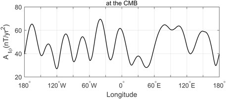
Figure 5. Average amplitude of time-latitude values of ΔSA-Br with the longitudes over the spherical surface at the CMB.

To study the time-latitude variation characteristics of ΔSA-Br, we plot the time-latitude diagrams of ΔSA-Br at the CMB based on the longitudes of the maxima and minima of A_tφ defined in Figure 5 (Figure 6). Since the ΔSA-Br values at longitudes with minima are relatively small, the distribution of positive and negative patches in the time-latitude diagrams is irregular. Consequently, we only show the time-latitude diagram at 120°W in the Western Hemisphere (Figure 6K) and that at 45°E in the Eastern Hemisphere (Figure 6L) as examples.

Figure 6

Figure 6. Time-latitude diagrams of ΔSA-Br at the CMB. Figures (A–J) (located at 166° W to 148°E) are the maximum value of the average amplitude of time-latitude values A_tφ, and (K, L) (located at 120°W and 45°E) are the minimum values of A_tφ, respectively.

It can be seen from Figure 6 that the time-latitude diagrams exhibit different variation characteristics between the Eastern and Western Hemispheres. In the Western Hemisphere, the time-latitude diagrams at 166°W, 136°W, 103°W, 73°W, 40°W, and 3°W primarily exhibit the following three characteristics: First, the positive and negative patches are mainly distributed near the equator. Second, the positive and negative patches alternate over time, with strong patches occurring around 2005, 2007, 2011, 2014, and 2017, which match the occurrence time of geomagnetic jerks. Moreover, the positive and negative patches occurring simultaneously exhibit reverse polarities for two adjacent circles of longitude. For example, the pulse patches corresponding to 2005, 2007, 2011, 2014, and 2017 have reverse positive and negative polarities between the two time-latitude diagrams at 40°W and 3°W (Figures 6E, F). The above phenomenon clearly shows that the polarities of pulse patches in the Western Hemisphere alternate over time, with polarity reversal occurring in the west-east direction.

In the Eastern Hemisphere, the distribution of patches in the time-latitude diagrams (Figures 6G–J) differs from that of patches in the time-latitude diagrams in the Western Hemisphere. The distribution of patches at 31°E (Figure 6G) and 80°E (Figure 6H) exhibits a larger span in the north-south direction, with relatively strong pulse patches still occurring near 40°S and 40°N. The polarities of the positive and negative patches occurring simultaneously do not have an evident reversal at these two longitudes. Similarly, the polarities of the positive and negative patches do not have an apparent reversal at 80°E and 105°E. The pulse patches at 148°E are near the equator (Figure 6J), with more intense pulses around 2014, 2017, and 2020 and positive and negative patches alternating over time. It can be seen from the comparison of the time-latitude diagrams, time-longitude diagrams (Figure 4A), and average magnetic flux diagrams (Figure 5) that the regions from 80°E to 105°E and near 148°E in the Eastern Hemisphere are two regions with the most active pulses.

4 Discussion

4.1 Amplitude of geomagnetic acceleration pulses and geomagnetic jerks

Figure 2 clearly shows that the occurrence time of the maxima of ΔSAA-Br at the CMB completely corresponds to the reported occurrence time of geomagnetic jerks occurring at the Earth’s surface, fully indicating that the amplitude of acceleration pulses at the CMB is a particularly sensitive parameter for identification of geomagnetic jerks. The average period of ∼3.2 years can be used as a new indicator for testing and predicting the occurrence time of geomagnetic jerks. It should be emphasized that the time series of the amplitude of acceleration pulses shown in Figure 2 is the global average effect, and it does not mean that geomagnetic jerks occur globally at the time with maxima occurring. Due to the geomagnetic field’s attenuation from the CMB to the Earth’s surface and the difference in distance for acceleration pulses from the CMB to the ground stations, the related geomagnetic jerks are a local phenomenon. They are not entirely synchronous at different positions at the Earth’s surface (Mandea et al., 2010). Therefore, a study on the relationship between acceleration pulses and geomagnetic jerks requires considering the global variation characteristics of acceleration pulses and the regional variation characteristics.

As pointed out above, the acceleration pulses have different variation characteristics between the Eastern and Western Hemispheres. To show the characteristics of the amplitude of acceleration pulses in different hemispheres, we calculate the intensities of geomagnetic acceleration pulses at the CMB in both Eastern and Western Hemispheres, respectively (Figure 7). We normalized all the data, and all the data were divided by the maximum value (1,660.5 nT/yr²), as shown in Figure 7. As can be discerned from Figure 7, the variations in amplitude are not wholly synchronous between the two hemispheres. In the years 2007.5 and 2011.0, there were maxima of the pulse amplitude occurring in both sector regions. However, the amplitude value in the Western Hemisphere was far more than that in the Eastern Hemisphere, and the corresponding jerks mainly occurred in the Western Hemisphere. For example, in these two years, no jerks occurred at the geomagnetic stations of the Chinese region. Still, only small secular variation fluctuations occurred (Kang et al., 2020), possibly because the acceleration pulses mainly happened in the Western Hemisphere, far from China. Around 2014, both hemispheres had similar amplitude values, and the corresponding jerks were global (Torta et al., 2015). In addition, around the years 2017.5 and 2020.3, the pulse amplitude values in the Eastern Hemisphere were more significant than those in the Western Hemisphere, indicating that the jerk events in these two years were dominated by the acceleration pulses in the Eastern Hemisphere (Whaler et al., 2020; Campuzano et al., 2021).

Figure 7

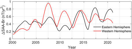
Figure 7. Variations in the amplitude of acceleration pulses at the CMB in the Eastern and Western Hemispheres over time.

4.2 Dynamic process of geomagnetic acceleration pulses at the CMB

The maxima of the amplitude of geomagnetic acceleration pulses are directly related to geomagnetic jerks, which can be obtained from Figures 2, 7. This suggests that the specific dynamic process of the Earth’s core is related to geomagnetic acceleration pulses. Time-longitude and time-latitude diagrams can only reflect the variations of acceleration pulses over time in the longitude and latitude directions. To comprehensively observe the dynamic variation process of acceleration pulses, we plot the distribution diagram of ΔSA-Br at the CMB (Figure 8) based on the epochs of maxima and minima of the pulse amplitude shown in Figure 2.

Figure 8

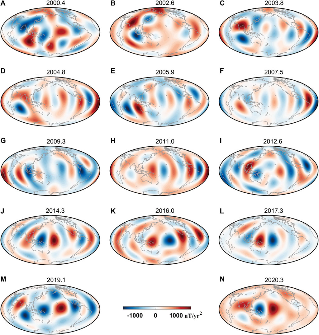
Figure 8. Variations of secular acceleration pulses of Br (ΔSA-Br) at the CMB. We use CHAOS-7.17 model until degree six to calculate the ΔSA-Br at the CMB for each 0.1 years during the last two decades. Panels (B,D,F,H,J,L,N) and (A,C,E,G,I,K,M) correspond to years with the maximum and minimum amplitudes.

It can be discerned from Figure 8 that, in several years before 2006, the pulse patches of ΔSA-Br deviated far away from the equator. In the Eastern Hemisphere, the pulse patches were mainly arranged along the north-south direction. In the years 2000.5 and 2003.8, with minima of pulse amplitude, the polarities of the positive and negative patches underwent reversal in the north-south direction. In the years 2002.6 and 2004.8 with maxima of pulse amplitude (i.e., the years with jerks occurring), the positions of the pulse patches varied greatly. However, the polarities of the positive and negative patches did not undergo an evident reversal. This may mean that the maximum pulse amplitude detected around 2005 does not entirely correspond to a “typical” geomagnetic jerk. Therefore, this maximum may correspond to a new characteristic of the geomagnetic field. Some scholars have reported and studied the jerk event around 2005 (Chulliat and Maus, 2014; Soloviev et al., 2017; Campuzano et al., 2021). Campuzano et al. (2021) believed that this is a geomagnetic jerk defined vaguely because it is too close to other jerks to be clearly distinguished from other jerks with routine tools. Chulliat and Maus (2014) also observed that the jerks around 2003 and 2005 were related to identical SA pulses. These jerks are defined vaguely and still need further study to confirm various possibilities.

It can be seen from Figure 8 that, in various years since 2006, the pulse patches were mainly located near the equator, and the positive and negative patches were primarily arranged along the west-east direction. Kloss and Finlay (2019) found that the equator area under the CMB has intense and local fluid motion. In addition, Finlay et al. (2016) found that the radial acceleration on the surface of the Earth’s core had strong oscillation in the equatorial area at 40°W. In the years 2007.5 and 2011, the patches mainly occurred in the Atlantic Ocean region of the Western Hemisphere. In 2014.3, the strongest patch happened in the Pacific Ocean region (Figure 8J); however, relatively strong patches occurred between 0° and 120°W in the Atlantic-America region. In 2017.3 and 2020.3, the pulse patches primarily happened in the middle Pacific Ocean region between 150°E and 150°W. The variations in pulse amplitude over time in the Eastern and Western Hemispheres shown in Figure 7 are determined by the geographic positions of the pulse patches.

The most significant variation characteristic of pulse patches since 2006 is that the polarities of the most extensive positive and negative patches undergo reversals in two adjacent years with maxima occurring (two years with adjacent jerks). For example, in 2007.5 and 2011.0, 2011.0 and 2014.3, 2014.3 and 2017.3, and 2017.3 and 2020.3, the polarities of patches exhibit evident reversal in the west-east direction. Polarity reversal occurs in transition periods with pulse amplitude reaching minima. Similarly, in two adjacent years, with minima of pulse amplitude occurring, the polarities of positive and negative patches also undergo reversal. This indicates that the jerks at the Earth’s surface are closely related to the polarity reversal of pulse patches. Chulliat and Maus (2014) noticed this characteristic of jerks occurring in 2007 and 2011 when studying the variation of signs of SA. Torta et al. (2015) reported the variations in signs of geomagnetic acceleration before and after the jerk occurring in 2014. Finlay et al. (2020) studied the evolution of the South Atlantic Anomaly and the rapid variation in the Pacific Ocean region after 2014. They found that the second derivative (the acceleration) of the radial component of the magnetic field underwent variation of the sign from 2015 to 2018 and pointed out that the variation in acceleration has a local dipole characteristic in the west-east direction. It originates from accelerated variations of the Earth’s core field in the low-latitude regions of the middle and western Pacific Ocean.

4.3 Causes of acceleration pulse variations

It can be seen from the above analyses that the amplitude of geomagnetic acceleration pulses at the CMB and the pulse patches exhibit consistent spatiotemporal evolution processes, indicating that the geomagnetic acceleration pulses exhibit significant differences between the Western and Eastern Hemispheres since 2000. This means that the dynamic process of the Earth’s core, which causes the variation of acceleration pulses, may have a characteristic of regional variation. In recent years, to explain the relationship between the rapid variation of the geomagnetic field with geomagnetic jerks, some scholars have reproduced the interaction between the Earth’s core convection and rapid magnetic fluid waves through numerical simulations (Buffett and Matsui, 2019; Aubert, 2020).

In this work, we have observed that the acceleration pulse patches are mainly distributed near the equator and exhibit alternating variation over time and polarity reversal in the west-east direction. These characteristics are similar to the rapid magnetic field fluctuation disclosed by the stratification model at the top of the Earth’s core (Pais et al., 2015; Buffett and Matsui, 2019; Gerick et al., 2021). Chulliat and Maus. (2014), Chulliat et al. (2015) analyzed the geomagnetic jerk events occurring in 2003, 2007, and 2011 and proposed that the jerks were caused by the standing waves occurring at the surface of the Earth’s core and centered around the low-latitude Atlantic plate, thus supporting the theoretical prediction about the assumption of stable stratification at the top of the Earth’s core by Bergman (1993). Based on the short-period fluctuations in geomagnetic acceleration recently found in satellite observation, Buffett and Matsui (2019) explained the observation result of rapid fluctuations in geomagnetic acceleration near the equator through numerical simulation of the interactions among the magnetic force, Archimedes force, and Coriolis force at the top layers of the Earth’s core.

The rapid fluctuations in geomagnetic acceleration generated by the zonal flows and geostrophic Alfvén waves in the Earth’s core can better show the characteristics of local acceleration pulse variations. Gillet et al. (2015) identified axisymmetric Alfvén waves with sub-decadal periods from the data from geomagnetic stations and satellites. Finlay et al. (2016) found that a series of outstanding axisymmetric azimuthal jet flows near the equator would undergo oscillations over time at some positions, which is consistent with the finding by Gillet et al. (2015). For example, at 40 ºW near the equator, intense oscillations of radial field SA can be observed at the surface of Earth’s core. These findings coincide with the result shown in Figure 3A that there are belts of dense maxima of acceleration pulses near the longitudes 40°W and 0°. Kloss and Finlay (2019) found, based on ground and satellite magnetic surveys that, since 2000, the sector regions from 60°W to 100°W and from 80°E to 130°E have undergone a series of characteristics of the strong azimuthal flow acceleration with sign alternating symbols exhibited. The region from 130°E to 150°W in the Pacific Ocean has also undergone strong azimuthal flow acceleration since 2012. They proposed that the quasi-geostrophic Alfvén waves may be an explanation for such events, and such waves are triggered in the deep part of the Earth’s core and propagated to the Earth’s core surface (Aubert and Finlay, 2019; Whaler et al., 2022). These explanations match robustly with the situations reflected by Figures 6, 8 that the acceleration pulse patches in the Eastern Hemisphere have larger spans in the north-south direction, and the pulses are more intense in the regions from 80°E to 105°E and near 148°E.

5 Conclusion

Our research results show that the amplitude series of the most extensive acceleration pulse patches are synchronous in variation between the Earth’s surface and the CMB, with a period of ∼3.2 years. We also found a connection between pulse amplitude and geomagnetic jerks, which has not been reported before. In other words, geomagnetic jerks occur in periods with pulse amplitude reaching its maximum. Therefore, pulse amplitude can be a sensitive and stable parameter for identifying and predicting a geomagnetic jerk.

The average amplitude of acceleration pulses at the CMB is asymmetric in north-south and west-east directions. In the north-south direction, the average amplitude reaches its maxima near the equator and its minima at two poles. In addition, there is still a maximum near 68°S in the Southern Hemisphere, and the variation in the Southern Hemisphere is more violent than that in the Northern Hemisphere. In the Western Hemisphere, the fluctuations of the average amplitude are relatively regular, with an average interval of 32°. In the Eastern Hemisphere, the variations in the average amplitude show no evident regularity, although the variation in the region from 80°E to 105°E is the most significant.

The polarity reversal, positions, and evolution of geomagnetic acceleration pulse patches over time have evident regional characteristics. During 2000–2006, the acceleration pulse patches in the Eastern Hemisphere were mainly arranged along the north-south direction, with relatively strong pulse patches still occurring near 40°N and 40°S. Since 2006, the positive and negative patches have been arranged along the west-east direction. The most significant characteristic of the pulse patches is that the polarities of the positive and negative patches undergo reversal in two years with adjacent jerks. Overall, in the Western Hemisphere, the pulse patches are located near the equator and exhibit an evident westward drifting characteristic. While the positive and negative patches exhibit alternating variation over time, the polarities of the patches undergo reversal in the west-east direction. These characteristics can be explained by the rapid magnetic field fluctuations disclosed by the model of stratification at the top of the Earth’s core. In the Eastern Hemisphere, the acceleration pulses are weaker from 10°E to 60°E. They are more active in the regions from 80°E to 105°E and near 150°E, exhibiting evident characteristics of local variation. These characteristics match the cases given by the zonal flow and geostrophic Alfvén waves in the Earth’s core.

We statistically analyze the maxima of the amplitude of geomagnetic acceleration pulses since 2000 by calculating the three-year difference in geomagnetic acceleration based on the CHAOS-7.17 geomagnetic field model and correspond the extrema to the occurrence time of the geomagnetic jerks. We analyze the dynamic variations of acceleration pulses based on the occurrence time of the maxima and minima of pulse amplitude. By calculating the average amplitude, we quantitatively determine the longitude and latitude distributions of the amplitude of acceleration pulses. Furthermore, based on the longitudes of the maxima of the average amplitude, we analyze the time-latitude variation of the acceleration pulses. With these methods, we can obtain clear images that can objectively reflect the spatiotemporal evolution characteristics of the acceleration pulses. Consequently, the new technique used in this paper is a promising tool for studying the variation in geomagnetic acceleration. The results obtained using this method can provide new information and bases for exploring the Earth’s core dynamic process of the evolution of acceleration pulses and for numerical geodynamo simulations.

Data availability statement

The original contributions presented in the study are included in the article/Supplementary Material, further inquiries can be directed to CB, YmFpY2hoQHludS5lZHUuY24=.

Author contributions

CB: Conceptualization, Data curation, Formal Analysis, Funding acquisition, Investigation, Methodology, Project administration, Resources, Software, Visualization, Writing–original draft, Writing–review and editing. GG: Data curation, Formal Analysis, Funding acquisition, Supervision, Validation, Writing–review and editing. LW: Data curation, Formal Analysis, Funding acquisition, Software, Supervision, Writing–review and editing. GK: Conceptualization, Data curation, Formal Analysis, Resources, Supervision, Writing–review and editing.

Funding

The author(s) declare that financial support was received for the research, authorship, and/or publication of this article. This work was funded by the National Natural Science Foundation of China (Grant Nos 42264005, 41964004) and Yunnan Fundamental Research Projects under contract (202101AT070181).

Acknowledgments

The results presented in this paper rely on geomagnetic field models of the CHAOS series and data collected at geomagnetic observatories. All data and models used to carry out this work can be found in the associated references and the repository of DTU Space (http://www.spacecenter.dk/files/magnetic-models/CHAOS-7/index.html). We thank the national institute(s) in charge of them and acknowledge the International Geomagnetic Network for facilitating the collection and dissemination of observatory data worldwide. We also thank the Editors and reviewers for their comments on the original manuscript.

Conflict of interest

The authors declare that the research was conducted in the absence of any commercial or financial relationships that could be construed as a potential conflict of interest.

Publisher’s note

All claims expressed in this article are solely those of the authors and do not necessarily represent those of their affiliated organizations, or those of the publisher, the editors and the reviewers. Any product that may be evaluated in this article, or claim that may be made by its manufacturer, is not guaranteed or endorsed by the publisher.

Supplementary material

The Supplementary Material for this article can be found online at: https://www.frontiersin.org/articles/10.3389/feart.2024.1383149/full#supplementary-material

References

Alken, P., Olsen, N., and Finlay, C. C. (2020). Co-estimation of geomagnetic field and in-orbit fluxgate magnetometer calibration parameters. Earth Planets Space 72, 49. doi:10.1186/s40623-020-01163-9

CrossRef Full Text | Google Scholar

Amit, H., Coutelier, M., and Christensen, U. R. (2018). On equatorially symmetric and antisymmetric geomagnetic secular variation timescales. Phys. Earth Planet. Inter. 276, 190–201. doi:10.1016/j.pepi.2017.04.009

CrossRef Full Text | Google Scholar

Amit, H., and Olson, P. (2006). Time-average and time-dependent parts of core flow. Phys. Earth Planet. Inter. 155, 120–139. doi:10.1016/j.pepi.2005.10.006

CrossRef Full Text | Google Scholar

Aubert, J. (2018). Geomagnetic acceleration and rapid hydromagnetic wave dynamics in advanced numerical simulations of the geodynamo. Geophys. J. Int. 214, 531–547. doi:10.1093/gji/ggy161

CrossRef Full Text | Google Scholar

Aubert, J. (2020). Recent geomagnetic variations and the force balance in Earth’s core. Geophys. J. Int. 221, 378–393. doi:10.1093/gji/ggaa007

CrossRef Full Text | Google Scholar

Aubert, J., and Finlay, C. C. (2019). Geomagnetic jerks and rapid hydromagnetic waves focusing at Earth’s core surface. Nat. Geosci. 12, 393–398. doi:10.1038/s41561-019-0355-1

CrossRef Full Text | Google Scholar

Aubert, J., Livermore, P., Finlay, C., Fournier, A., and Gillet, N. (2022). A taxonomy of simulated geomagnetic jerks. Geophys. J. Int. 231, 650–672. doi:10.1093/gji/ggac212

CrossRef Full Text | Google Scholar

Barrois, O., Gillet, N., and Aubert, J. (2017). Contributions to the geomagnetic secular variation from a reanalysis of core surface dynamics. Geophys. J. Int. 211 (1), 50–68. doi:10.1093/gji/ggx280

CrossRef Full Text | Google Scholar

Bergman, M. I. (1993). Magnetic Rossby waves in a stably stratified layer near the surface of the Earth’s outer core. Geophys. Astrophysical Fluid Dyn. 68 (1-4), 151–176. doi:10.1080/03091929308203566

CrossRef Full Text | Google Scholar

Brown, W., and Mound, J. L. P. (2013). Jerks abound: an analysis of geomagnetic observatory data from 1957 to 2008. Phys. Earth Planet. Inter. 223, 62–76. doi:10.1016/j.pepi.2013.06.001

CrossRef Full Text | Google Scholar

Buffett, B., and Matsui, H. (2019). Equatorially trapped waves in Earth’s core. Geophys. J. Int. 218 (2), 1210–1225. doi:10.1093/gji/ggz233

CrossRef Full Text | Google Scholar

Campuzano, S. A., Pavón-Carrasco, F. J., De Santis, A., González-López, A., and Qamili, E. (2021). South Atlantic Anomaly areal extent as a possible indicator of geomagnetic jerks in the satellite era. Front. Earth Sci. 8, 607049. doi:10.3389/feart.2020.607049

CrossRef Full Text | Google Scholar

Chulliat, A., Alken, P., and Maus, S. (2015). Fast equatorial waves propagating at the top of the Earth’s Core. Geophys. Res. Lett. 42 (9), 3321–3329. doi:10.1002/2015GL064067

CrossRef Full Text | Google Scholar

Chulliat, A., and Maus, S. (2014). Geomagnetic secular acceleration, jerks, and a localized standing wave at the core surface from 2000 to 2010. J. Geophys. Res. Solid Earth. 119 (3), 1531–1543. doi:10.1002/2013JB010604

CrossRef Full Text | Google Scholar

Chulliat, A., Thébault, E., and Hulot, G. (2010). Core field acceleration pulse as a common cause of the 2003 and 2007 geomagnetic jerks. Geophys. Res. Lett. 37 (7), L07301. doi:10.1029/2009GL042019

CrossRef Full Text | Google Scholar

Constable, C., Korte, M., and Panovska, S. (2016). Persistent high paleosecular variation activity in southern hemisphere for at least 10 000 years. Earth Planet. Sci. Lett. 453, 78–86. doi:10.1016/j.epsl.2016.08.015

CrossRef Full Text | Google Scholar

Finlay, C. C., Kloss, K., Olsen, N., Hammer, M. D., Toffner-Clausen, L., Grayver, A., et al. (2020). The CHAOS-7 geomagnetic field model and observed changes in the South Atlantic Anomaly. Earth Planets Space 72, 156. doi:10.1186/s40623-020-01252-9

PubMed Abstract | CrossRef Full Text | Google Scholar

Finlay, C. C., Olsen, N., Kotsiaros, S., Gillet, N., and Tøffner-Clausen, L. (2016). Recent geomagnetic secular variation from Swarm and ground observatories as estimated in the CHAOS-6 geomagnetic field model. Earth Planets Space 68, 112. doi:10.1186/s40623-016-0486-1

CrossRef Full Text | Google Scholar

Gerick, F., Jault, D., and Noir, J. (2021). Fast quasi-geostrophic magneto-coriolis modes in the Earth’s core. Geophys. Res. Lett. 48 (4), E2020GL090803. doi:10.1029/2020GL090803

CrossRef Full Text | Google Scholar

Gillet, N., Huder, L., and Aubert, J. (2019). A reduced stochastic model of core surface dynamics based on geodynamo simulations. Geophys. J. Int. 219 (1), 522–539. doi:10.1093/gji/ggz313

CrossRef Full Text | Google Scholar

Gillet, N., Jault, D., and Finlay, C. C. (2015). Planetary gyre, time-dependent eddies, torsional waves, and equatorial jets at the Earth's core surface. J. Geophys. Res. Solid Earth. 120 (6), 3991–4013. doi:10.1002/2014JB011786

CrossRef Full Text | Google Scholar

Holme, R., Olsen, N., and Bairstow, F. L. (2011). Mapping geomagnetic secular variation at the core-mantle boundary. Geophys. J. Int. 186 (2), 521–528. doi:10.1111/j.1365-246X.2011.05066.x

CrossRef Full Text | Google Scholar

Kang, G. F., Gao, G. M., Wen, L. M., and Bai, C. H. (2020). The 2014 geomagnetic jerks observed by geomagnetic observatories in China. Chin. J. Geophys 63 (11), 4144–4153. doi:10.6038/cjg2020N0337

CrossRef Full Text | Google Scholar

Kloss, C., and Finlay, C. C. (2019). Time-dependent low-latitude core flow and geomagnetic field acceleration pulses. Geophys. J. Int. 217 (1), 140–168. doi:10.1093/gji/ggy545

CrossRef Full Text | Google Scholar

Kotzé, P. B. (2017). The 2014 geomagnetic jerk as observed by southern African magnetic observatories. Earth Planets Space 69, 17. doi:10.1186/s40623-017-0605-7

CrossRef Full Text | Google Scholar

Kotzé, P. B., and Korte, M. (2016). Morphology of the southern African geomagnetic field derived from observatory and repeat station survey observations: 2005-2014. Earth Planets Space 68, 23. doi:10.1186/s40623-016-0403-7

CrossRef Full Text | Google Scholar

Lesur, V., Gillet, N., Hammer, M. D., and Mandea, M. (2022). Rapid variations of Earth’s core magnetic field. Surv. Geophys. 43, 41–69. doi:10.1007/s10712-021-09662-4

CrossRef Full Text | Google Scholar

Lesur, V., Wardinski, I., Baerenzung, J., and Holschneider, M. (2018). On the frequency spectra of the core magnetic field gauss coefficients. Phys. Earth Planet. Inter. 276, 145–158. doi:10.1016/j.pepi.2017.05.017

CrossRef Full Text | Google Scholar

Livermore, P., Hollerbach, R., and Finlay, C. (2017). An accelerating high-latitude jet in Earth’s core. Nat. Geosci. 10, 62–68. doi:10.1038/ngeo2859

CrossRef Full Text | Google Scholar

Mandea, M., Holme, R., Pais, A., Pinheiro, K., Jackson, A., and Verbanac, G. (2010). Geomagnetic jerks: rapid core field variations and core dynamics. Space Sci. Rev. 155, 147–175. doi:10.1007/s11214-010-9663-x

CrossRef Full Text | Google Scholar

Metman, M. C., Beggan, C. D., Livermore, P. W., and Mound, J. E. (2020). Forecasting yearly geomagnetic variation through sequential estimation of core flow and magnetic diffusion. Earth Planets Space 72, 149. doi:10.1186/s40623-020-01193-3

CrossRef Full Text | Google Scholar

Nahayo, E., and Korte, M. (2022). A regional geomagnetic field model over Southern Africa derived with harmonic splines from Swarm satellite and ground-based data recorded between 2014 and 2019. Earth Planets Space 74, 8. doi:10.1186/s40623-021-01563-5

CrossRef Full Text | Google Scholar

Olsen, N., Lühr, H., Finlay, C. C., Sabaka, T. J., Michaelis, I., Rauberg, J., et al. (2014). The CHAOS-4 geomagnetic field model. Geophys. J. Int. 197 (2), 815–827. doi:10.1093/gji/ggu033

CrossRef Full Text | Google Scholar

Olsen, N., Lühr, H., Sabaka, T. J., Mandea, M., Rother, M., Tøffner-Clausen, L., et al. (2006). CHAOS-a model of the Earth's magnetic field derived from CHAMP, Ørsted, and SAC-C magnetic satellite data. Geophys. J. Int. 166 (1), 67–75. doi:10.1111/j.1365-246X.2006.02959.x

CrossRef Full Text | Google Scholar

Olsen, N., and Mandea, M. (2007). Investigation of a secular variation impulse using satellite data: the 2003 geomagnetic jerk. Earth Planet. Sci. Lett. 255 (1-2), 94–105. doi:10.1016/j.epsl.2006.12.008

CrossRef Full Text | Google Scholar

Olsen, N., Mandea, M., Sabaka, T. J., and Tøfner-Clausen, L. (2009). CHAOS-2-A geomagnetic field model derived from one decade of continuous satellite data. Geophys. J. Int. 179 (3), 1477–1487. doi:10.1111/j.1365-246X.2009.04386.x

CrossRef Full Text | Google Scholar

Ou, J. M., Du, A. M., and Xu, W. Y. (2016). Investigation of the SA evolution by using the CHAOS-4 model over 1997-2013. Sci. China Earth Sci. 59 (5), 1041–1050. doi:10.1007/s11430-016-5265-0

CrossRef Full Text | Google Scholar

Pais, M. A., Morozova, A. L., and Schaeffer, N. (2015). Variability modes in core flows inverted from geomagnetic field models. Geophys. J. Int. 200 (1), 402–420. doi:10.1093/gji/ggu403

CrossRef Full Text | Google Scholar

Pavón-Carrasco, F. J., and De Santis, A. (2016). The South Atlantic anomaly: the key for a possible geomagnetic reversal. Front. Earth Sci. 4, 40. doi:10.3389/feart.2016.00040

CrossRef Full Text | Google Scholar

Pavón-Carrasco, F. J., Marsal, S., Campuzano, S. A., and Torta, J. M. (2021). Signs of a new geomagnetic jerk between 2019 and 2020 from Swarm and observatory data. Earth Planets Space 73, 175. doi:10.1186/s40623-021-01504-2

CrossRef Full Text | Google Scholar

Pinheiro, K. J., Jackson, A., and Finlay, C. C. (2011). Measurements and uncertainties of the occurrence time of the 1969, 1978, 1991, and 1999 geomagnetic jerks. Geochem. Geophys. Geosys. 12 (10), Q10015. doi:10.1029/2011GC003706

CrossRef Full Text | Google Scholar

Sabaka, T. J., Toffner-Clausen, L., Olsen, N., and Finlay, C. C. (2020). CM6: a comprehensive geomagnetic field model derived from both CHAMP and Swarm satellite observations. Earth Planets Space 72, 80. doi:10.1186/s40623-020-01210-5

CrossRef Full Text | Google Scholar

Soloviev, A., Chulliat, A., and Bogoutdinov, S. (2017). Detection of secular acceleration pulses from magnetic observatory data. Phys. Earth Planet. Inter. 270, 128–142. doi:10.1016/j.pepi.2017.07.005

CrossRef Full Text | Google Scholar

Stefan, C., Dobrica, V., and Demetrescu, C. (2017). Core surface sub-centennial magnetic flux patches: characteristics and evolution. Earth Planets Space 69, 146. doi:10.1186/s40623-017-0732-1

CrossRef Full Text | Google Scholar

Torta, J. M., Pavón-Carrasco, F. J., Marsal, S., and Finlay, C. C. (2015). Evidence for a new geomagnetic jerk in 2014. Geophys. Res. Lett. 42 (19), 7933–7940. doi:10.1002/2015GL065501

CrossRef Full Text | Google Scholar

Whaler, K., Hammer, M. D., Finlay, C., and Olsen, N. (2020). Core-mantle boundary flows obtained purely from Swarm secular variation gradient information. EGU General Assem., 2020. doi:10.5194/egusphere-egu2020-9616

CrossRef Full Text | Google Scholar

Whaler, K. A., Hammer, M. D., Finlay, C. C., and Olsen, N. (2022). Core surface flow changes associated with the 2017 Pacific geomagnetic jerk. Geophys. Res. Lett. 49 (15), e2022GL098616. doi:10.1029/2022GL098616

PubMed Abstract | CrossRef Full Text | Google Scholar

Xu, W. Y. (2009). Physics of electromagnetic phenomena of the Earth. Hefei: University of Science and Technology of China Press, 140–141. (in Chinese).

Google Scholar