 D. Prekrat
 N. K. Todorović-Vasović1
 S. Kostić
94% of researchers rate our articles as excellent or good
Learn more about the work of our research integrity team to safeguard the quality of each article we publish.
Find out more
ORIGINAL RESEARCH article
Front. Earth Sci., 19 March 2024
Sec. Geohazards and Georisks
Volume 12 - 2024 | https://doi.org/10.3389/feart.2024.1374942
This article is part of the Research TopicContemporary Characterization and Modeling of Earth Processes: A Multidisciplinary ApproachView all 4 articles
In the present paper, we investigate the effect of the initial conditions on the dynamics of the spring-block landslide model. The time evolution of the studied model, which is governed by a system of stochastic delay differential equations, is analyzed in the mean-field approximation, which qualitatively exhibits the same dynamics as the initial model. The results of the numerical analysis show that changing the initial conditions has different effects in different parts of the parameter space of the model. Namely, moving away from the fixed-point initial conditions has a stabilizing effect on the dynamics when the noise, the friction parameters a (higher values) and c as well as the spring stiffness k are taken into account. The stabilization manifests itself in a complete suppression of the unstable dynamics or a partial limitation of the effect of some friction parameters. On the other hand, the destabilizing effect of changing the initial conditions occurs for the lower values of the friction parameters a and for b. The main feature of destabilization is the complete suppression of the sliding regime or a larger parameter range with a transient oscillatory regime. Our approach underlines the importance of analyzing the influence of initial conditions on landslide dynamics.
Under natural conditions, slopes can generally be found in different dynamic states: (group 1) stable slopes with no prior or current movement, (group 2) creeping slopes, which exhibit permanent small displacements, with periodic intermittent sudden increases in the movement of the whole slope or some parts of the slope, and (group 3) the so-called conditionally stable slopes, whose stability strongly depends on their initial conditions. From the point of view of nonlinear dynamics, the conditions that leads to the instability of stable slopes (group 1) were first studied by Davis (1992), who initially proposed that the dynamics of the two-block system sliding on an inclined slope can be described by a system of three ordinary differential equations. In particular, Davis (1992) proposed such a model for certain classes of debris flows to explain the episodic surge motions. However, he was unable to estimate the onset of surging because he could not accurately determine the interaction between the steep feeder section of the slope and the lower and flatter accumulation section of the slope. In this paper, Davis (1992) assumed a velocity-dependent frictional force and suggested that there is a time delay between the movement of the feeder and the accumulation section of the slope. Our previous research, Kostić et al. (2023b), Kostić et al. (2023a), and Kostić and Stojković (2023) started from the model by Davis (1992) and introduced the explicit effect of time delay and random background noise Kostić et al. (2023b), with variable friction law Kostić et al. (2023a) and under the influence of river level oscillations, which were modeled as an external effect of colored noise Kostić and Stojković (2023). In the paper Kostić et al. (2023b) we first justified the introduction of random noise into a landslide model based on the results of recorded ambient noise within an existing landslide in Serbia. The results of further analysis showed that the background noise has a positive effect on the dynamics of the landslide, i.e., the increase in noise intensity requires a lower deformability of the slope and a higher displacement delay for bifurcation to occur. This confirms the positive stabilizing effect of increasing the noise intensity on the dynamics of the analyzed landslide model. In Kostić et al. (2023a), we first excluded the presence of significant noise in the observed landslide displacement. In a further analysis, we examined the effects of delayed failure and different friction laws on the change of dynamic regimes. It appears that under homogeneous geological conditions, sliding stabilizes with the increase of friction parameters, while rapid irregular sliding along the slope occurs with the increase of certain friction parameters. In the paper Kostić and Stojković (2023) we first show that the noise part of the deterministic model for the oscillation of the Kolubara River and the Ibar River (Serbia) has the properties of colored noise. In further analysis, it is found that landslide dynamics is sensitive to the change in noise intensity and that the increase in noise intensity leads to the onset of unstable landslide dynamics, while landslide dynamics is rather robust to the change in correlation time ϵ.
Concerning the dynamics of creeping slopes (group 2), some initial studies on creeping slopes were carried out by Chau (1995), who proposed a system of first-order ordinary differential equations, but where friction depends on both on the rate and state (Dieterich-Ruina friction law). This model is proposed for creeping slopes, and Chau (1995) investigated the specific bifurcation that can occur in the analyzed dynamical system depending on the state parameters of the sliding surface. He also showed that a small perturbation can lead to instability of the previously stable slope. Our earlier work Kostić et al. (2014) built on the work of Chau (1995) and further investigated the role of time delay in the emergence of deterministic chaos in the model of landslide dynamics. In particular, we investigated the dynamics of a single-block model on an inclined slope with Dieterich–Ruina friction law under the variation of two time delays and the initial shear stress, assuming that a periodic perturbation of the initial shear stress mimics the external triggering effect of long-distance earthquakes or some non-natural vibration source. The results obtained show conditions under which complex landslide dynamics occur, with a complete Ruelle–Takens–Newhouse route to deterministic chaos.
Chau (1999) also investigated the creeping slope model, in which friction depends on two state variables. Chau applied Reyn’s stability classification for the three-dimensional space and showed that the change of the nonlinear parameters of the slip surface, which can be triggered by rainfall or human activities, causes the occurrence of bifurcations in the studied dynamical system. One conclusion of his research is that, assuming a two-state variable friction law, the weakening of the velocity observed in the laboratory does not necessarily imply an unstable creeping slope with the same slip surface in the field (in the case of an infinite slope), while an amplification of the velocity does not necessarily imply a stable slope with the same slip surface. On the other hand, Qin et al. (2002) has proposed a nonlinear dynamical model for landslide evolution in the form of a system of three first-order nonlinear differential equations, where stress, displacement and precipitation change over time. The proposed model was applied to the case study of Xintan landslide, successfully reproducing the observed data.
The third dynamical state of the natural slope, i.e., conditionally stable slopes, has not been investigated so far. From a purely theoretical point of view, dynamic systems are in some cases sensitive to the change of initial conditions, i.e., this change can lead to the occurrence of global bifurcations Fuentes et al. (2011). We have already investigated such sensitivity from the point of view of theoretical neurology Franović et al. (2016). In the present work, we investigate the effect of changing the initial conditions on the onset of a complex dynamical behavior, which is supposed to correspond to an active landslide movement.
From an engineering point of view, landslides are indeed sensitive to changes in the original soil conditions. For example, Schilirò et al. (2019) conducted various flume tests in order to investigate the triggering process of rainfall-induced shallow landslides, focusing on the role of initial hydraulic conditions by changing the slope. They found that at a slope of 35°, the initial water content increases before the triggering occurs. This result and the lack of failure at gradient of 27° indicate the remarkable sensitivity of the tested material to even small variations in gradient. The data derived from the pore water pressure and soil moisture sensors point to two potential trigger mechanisms for variations in initial water content, namely, the advance of the wetting front at relatively high initial soil moisture content and the rise of a temporary perched water table, respectively, in relation to the failure mode. In general, the triggering of landslides was suggested to be strongly dependent on the initial water content and the initial slope angle. Also, initial porosity of the soil was already pointed out by Iverson et al. (2000) as an important initial condition for the occurrence of very different landslide rates. In their research, they raise a simple question: Can small differences in initial conditions cause some landslides to accelerate catastrophically and others to creep downslope only intermittently? Their analysis shows that landslides with a rate of 1 m/s can be triggered in moist sandy soil with a porosity of about 0.5, while the landslide rate drops to 0.002 m/s for the same soil with a porosity of about 0.4. Similar conclusions were drawn by Iverson et al. (2015), whose results from the Oso 2014 landslide indicate the primary dependence of landslide mobility on initial water content, initial porosity and initial sediment conditions.
Numerous previous studies have examined the stability of rock and soil slopes under various conditions, employing diverse models and utilizing a range of analytical, numerical and experimental methodologies (Xu et al., 2017; Zhang and Zhou, 2018; Zhou and Chen, 2019; Cheng et al., 2021; Shou et al., 2022; Li et al., 2023). In the present work, we start from the phenomenological spring-block model of Davis (1992), introduce a time delay and assume a velocity-dependent friction law proposed by Morales et al. (2017). We then simulate the model numerically and investigate how it behaves under the change of initial conditions. The paper is organized as follows. Section 2 provides a description of the investigated model. The methodology, results and related discussion can be found in Section 3, while Section 4 is dedicated to the main conclusions and directions for further research.
Let us consider a spring-block model on an inclined plane with angle θ, consisting of block-units with mass δm connected by springs with stiffness κδm and natural length δl which are acted upon by friction F(v)δm
A steady-state motion with sliding velocity v is achieved when the tangential component of gravity is balanced by friction, as the spring effects within the block cancel each other out:
This means that in the simplest case of a general motion of the block-unit i with the position pi and the velocity vi, Newton’s second law
reduces to
We will now proceed as in Vasović et al. (2016). If we go beyond the nearest-neighbor interaction, introduce a spring-effect delay τ and a Wiener noise d-term, and switch to a unit’s displacement xi and velocity yi = vi − v relative to the steady-state values, we can model our system of block-units by the following stochastic delay differential equation:
Here subscript τ indicates that the quantity is evaluated at t − τ.
After applying the mean-field (MF) approximation to Eq. 5 (see Supplementary Appendix), we obtain the following system that describes our spring-block model.
The system follows the time evolution of the MF variables.
• mx–mean displacement of the block elements,
• my–mean displacement velocity of the block elements,
• sx–variance of the displacement of the block elements,
• sy–variance of the displacement velocity of the block elements,
• u–cross-variance between the displacement and displacement velocity of the block elements,
under the influence of the following parameters.• a, b, c–friction parameters,
• d–noise,
• k–spring stiffness.
The friction in our model is given by
where the default values of the parameters are
and is shown in Figure 1. Since we would like to track the behavior of the system when the friction parameters are varied individually, positivity of the friction for the default sliding velocity F (v = 0.1) > 0 puts the following restrictions on the intervals of the friction parameters:
If we wish the friction to keep the same shape (as a function of v), the friction parameters must also fulfill the following conditions:
• a > 0 so that F(v) generally increases with v;
• F(v) must have a local maximum followed by a local minimum.
The second condition means that F′(v) = 3av2 − 2bv + c = 0 has two real solutions,which is fulfilled if b2 > 3ac. The parameter constraints (9) are now changed to:
For v± > 0 to apply, it must hold b > 0 and ac > 0. Also, if v− is a local maximum and v+ a local minimum, we must have F″(v−) < 0 and F″(v+) > 0, which is automatically satisfied. Finally, we wish to have F (v+) > 0, which yields b2 < 4ac and therefore
This further restricts our intervals to:
A deviation from these intervals would not automatically invalidate our model (e.g., our default v is not close to v+, so small parameter changes would not necessarily be affected by F (v+) < 0), but would certainly require special attention.
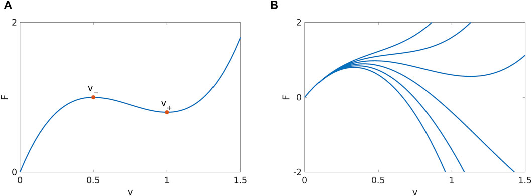
Figure 1. (A) Friction function F(v) = av3− bv2+ cv for a= 3.2, b= 7.2 and c= 4.8. Our default value for the sliding velocity v= 0.1 lies in the nearly linear part of the friction function. (B) Change of friction shape under variation of a (a=0, 1, 2, 3, 4, 5, from bottom to top).
Let us now find fixed points of system (6a)–(6e) describing the time evolution of our model. Equating all time derivatives to 0 immediately leads to my = 0 and u = 0 ((6a) and (6c)). Furthermore, dmx = 0 implies mx,τ = mx, so that the delay term in (6b) disappears. This leaves us with the following system for the fixed point:
For k = 0 the system is solved by sy = 0 provided that d = 0. For k > 0 we have sx = sy/k and.
If 3av − b ≠ 0, as satisfied by the default values of the friction parameters and sliding velocity, the system is again solved by sy = 0 and d = 0. However, if 3av − b = 0, a second non-trivial fixed point with
appears, which can be simplified into
Since sx, sy ≠ 0, this fixed point presumably corresponds to oscillations within the system that do not affect the motion of the center of mass. For the default friction parameters, the second fixed point appears for v = b/(3a) = 0.75. As we can see from (10), this value lies in the middle of the interval between v− and v+, in which the friction shows a weak dependence on the sliding velocity. It is interesting to note that our friction law has up to three sliding solutions for the same friction value in a certain range of inclination angles. The behavior of the system in this regime could be an interesting topic for further research.
We will examine the behavior of the system around the fixed point:
For the sake of simplicity, we introduce an offset parameter δ and look at the initial conditions
and d ≠ 0. A system with d ≪ 1 and δ ≪ 1 is considered to be near the fixed point.
System (6a)–(6e) was solved numerically in MATLAB using the forward Euler method with time step dt = 0.001 for a dense selection of system parameters and a wide range of initial conditions δ. The late-time series of solutions were then automatically classified as describing (asymptotically) sliding, oscillatory or complex oscillatory regime. The classification was done by looking at the time series in a window t ∈ [99000, 100000]. Examples of solutions in these regimes are shown in Figure 2. The solution is classified as unstable if the oscillation amplitude increases exponentially and reaches numerical infinity within a very short time, which terminates the numerical simulation.
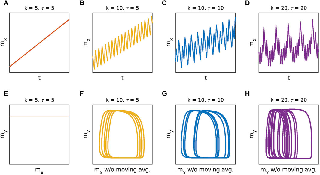
Figure 2. Examples of time series for solutions in each of the detected regimes—sliding (A), oscillatory (B), and complex oscillatory regime (C,D). The subfigures (E–H) show the corresponding phase portraits for the time series (A–D). Their respective Lyapunov exponents are 1.4 (9)⋅10–6, 0.011 (6), −0.007 (19), −0.03 (2), and they are consistent with the value 0. The system parameters for these examples are: a = 3.2, b = 7.2, c = 4.8, d = 10–4, v = 0.1.
We see from Figure 2 that mx generally increases with time, indicating a higher sliding velocity than the assumed steady-state value v or perhaps landslide straining. It is important to note that this change δv is typically orders of magnitude smaller than the sliding velocity v. In the sliding regime, the effect disappears when we remove the noise d. However, this is not the case in the oscillating regimes. A possible explanation could also be the non-isotropic friction law. Indeed, if the friction parameter b is switched off, the effect is drastically reduced and often even completely eliminated. The interaction with other parameters of the system, such as the delay time, deserves further investigation.
The regime of complex oscillations is considered as a phenomenological model of landslide dynamics. It is particularly interesting because it can manifest itself in various different forms. Period-doubling is the simplest example of this regime (Figure 2C). The doubling is clearly visible when comparing the phase portraits in Figure 2F and Figure 2G. More complicated examples of complex oscillations such as stick-slip and pulse-like oscillations can be seen in Figure 3.
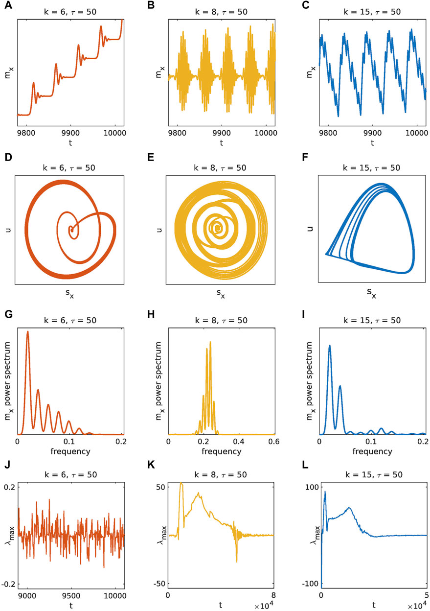
Figure 3. Examples of the complex oscillatory regime with large delay for a = 3.2, b = 7.2, c = 4.8, d = 10–4, v = 0.1, and initial conditions with offset δ = 10–4. The figure rows contain time series (A–C), phase portraits (D–F), power spectra (G–I), and Lyapunov exponents (J–L). The Lyapunov exponents (J), (K), and (L) converge to
After recognizing the possible solution types, we independently varied all parameters of the system and investigated their influence on the extent of the different regimes in the parameter space of the system. We performed this analysis both near and away from the fixed point of the system in order to work out the separate influence of the initial conditions on the dynamics of the landslide.
When analyzing in detail the transition between the different dynamical regimes of the landslide model under study (Figure 4), it becomes clear that a Ruelle-Takens-Newhouse route to deterministic chaos occurs. We start with stable sliding at low values of k and τ. As the control parameters are increased, an oscillatory regime first appears through a direct Hopf bifurcation, followed by a period-doubling bifurcation and finally the emergence of a complex oscillatory regime.
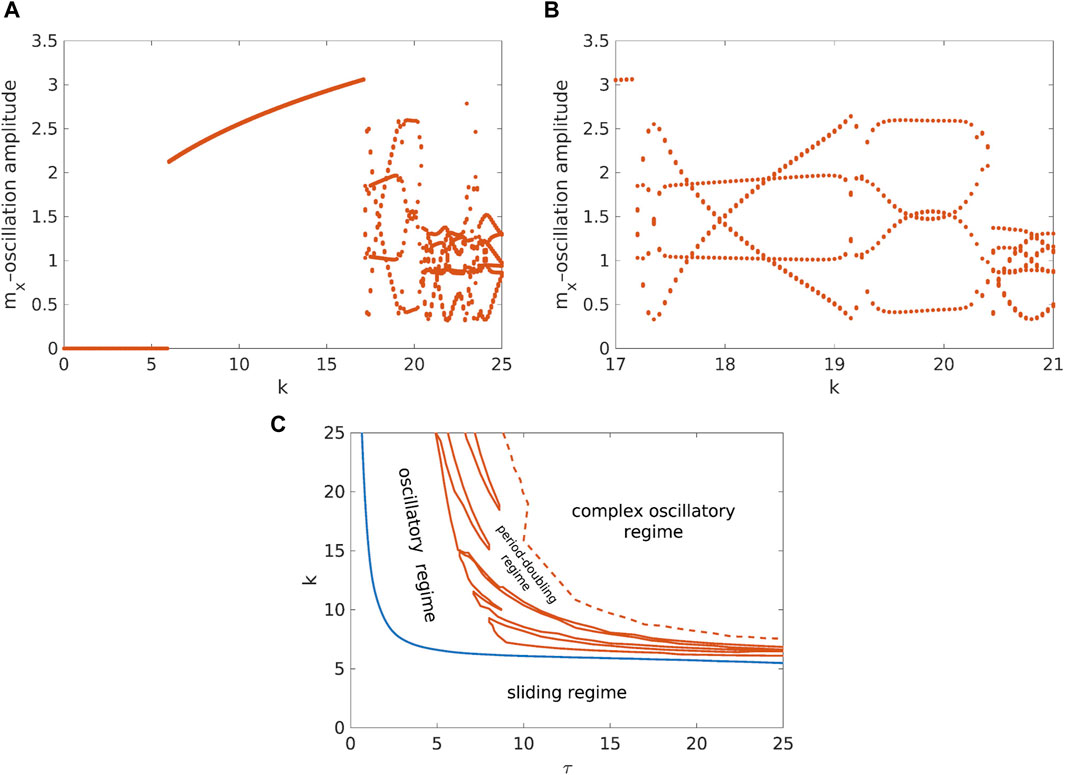
Figure 4. (A,B) Bifurcation of the oscillation amplitude for a = 3.2, b = 7.2, c = 4.8, d = 10–4, v = 0.1, τ = 10, and initial conditions with offset δ = 10–1. Plot (A) clearly shows sliding (k ≲6), oscillatory (6≲ k ≲17) and complex oscillatory regime (k ≳17). Plot (B) in addition shows zoomed-in region in which period-doubling appears—up to about k = 20.5, there are four distinct amplitudes for each k, which is consistent with the period-doubling time series in Figure 2C. (C) Phase diagram for a = 3.2, b = 7.2, c = 4.8, d = 10–4, v = 0.1, with initial conditions δ = 10–6, showing the onset of the period-doubling within the complex oscillatory regime.
The role of k and τ could be further investigated for very high values of τ. We have found that for extremely high values of τ, the change of k leads to a regular periodic stick-slip behavior. Nevertheless, it should be noted that such behavior could be considered transient, at least in some cases, since the widening of the investigated time window transforms the regular periodic stick-slip behavior into regular pulse-like oscillations.
As for the change in initial conditions, it has the following effects on the dynamics of the studied landslide model under investigation. From the point of view of spring stiffness, i.e., the deformability of the slope, and the time delay, distant initial conditions “stabilize” the landslide dynamics (Figure 5). In particular, when the initial conditions are away from the fixed point, a complex oscillatory regime is pushed towards higher values of k and τ.
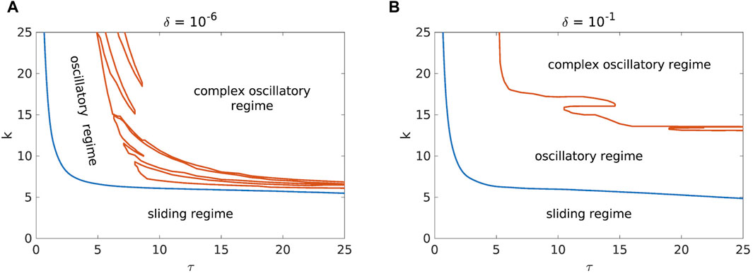
Figure 5. Comparison of the phase diagrams for a = 3.2, b = 7.2, c = 4.8, d = 10−4, v = 0.1 and with initial conditions near [(A), δ = 10−6] and far [(B), δ = 10−1] from the fixed point.
Let us now present some analytical arguments for the qualitative behavior of the transition between the sliding and the oscillatory regime in the (k, τ)-diagram for small τ. Since my = dmx/dt, the oscillations in mx should also be reflected in oscillations in my, therefore we can consider Eq. 6b. Firstly, assuming that the amplitude of the oscillations is small, we can disregard higher powers of my. Secondly, the amplitude of sy oscillations is typically orders of magnitude smaller than that of my, so we can also disregard sy-terms which yields
If we consider the small τ regime and remember that my = dmx/dt, we can expand mx,τ = mx (t − τ) as follows
which transforms (20), up to O (τ4), into a second-order linear differential equation
If the discriminant of its characteristic polynomial
is negative, we can expect an oscillating solution, and if it is positive, a sliding solution. The discriminant can be further rewritten as a quadratic polynomial in kτ2:
which has one positive zero
that is
which defines the boundary between the sliding and the oscillating regime. For the data used in Figure 6A, this boundary is well fitted by
We see that (26) only qualitatively explains the sharp drop of the transition line in Figure 5 between these two regimes for small τ. It also explains the nearly vertical small-delay transition line in Figure 6 and Figure 9. Namely, since the leading term in (26) does not depend on the friction parameters, a constant k leads to a nearly constant τ, regardless of the changes in the friction parameters. This applies in particular to a, as it has the least influence on F′(v).
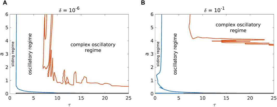
Figure 6. Comparison of the phase diagrams for b= 7.2, c= 4.8, d= 10−4, k= 12, v= 0.1 and with initial conditions near [(A), δ= 10−6] and far [(B), δ= 10−1] from the fixed point.
As far as the effect of the friction parameters is concerned, the influence of the variation of the higher values of the parameter a is similar to the effect of the slope deformability (Figure 6). However, at very low values of the parameter a, a new dynamical regime appears, namely, the unstable regime (Figure 7). The investigated system exhibits such dynamics regardless of the values of the time delay for the values of the parameter a in the range of 0.03–0.04. The influence of the initial conditions can further destabilize the dynamics of the landslide, i.e., the sliding regime with small time delay (Figure 7B) “vanishes” when the initial conditions are away from the fixed point. It should be noted that low values of a are far outside the reasonable parameter intervals (13a)–(13c), so it is possible that the unstable regime is caused by a velocity feedback loop where the system is accelerated by the increasing “unnatural” negative friction. Other parameters have also been considered at low values, but a has received more attention because its phase transition line is at low values.
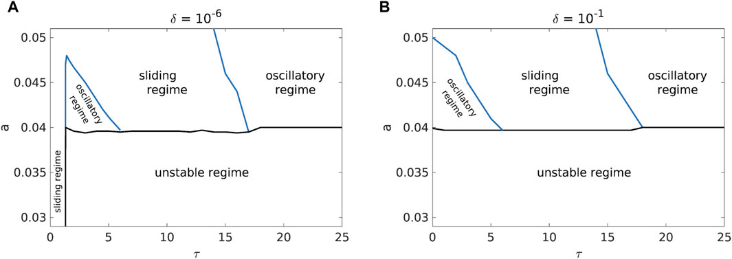
Figure 7. Comparison of the phase diagrams for b = 7.2, c = 4.8, d = 10−4, k = 12, v = 0.1 and with initial conditions near [(A), δ = 10−6] and far [(B), δ = 10−1] from the fixed point.
Turning to the next friction parameter, it turns out that shifting the initial conditions away from the fixed point interacting with b destabilizes the dynamics of the landslide. Indeed, the oscillatory regime occurs at much lower values of b and τ when δ is closer to 0. Moreover, at higher values of b, the system enters a mixed sliding/oscillatory regime, the extent of which is largely independent of the initial conditions (Figure 8). Here, even a small change in b or τ can cause the “random” switching between the oscillatory and the sliding regime. If we look closer at Figure 8C, we see that in the case of the mixed regime λmax remains positive even for very long but finite time series and only converges asymptotically to 0. This could perhaps explain the “chaotic” nature of the mixed regime. This is also in contrast to other regimes where λmax ends up oscillating tightly around 0 within a finite time (Figure 3J–L; Figures 8D, E).
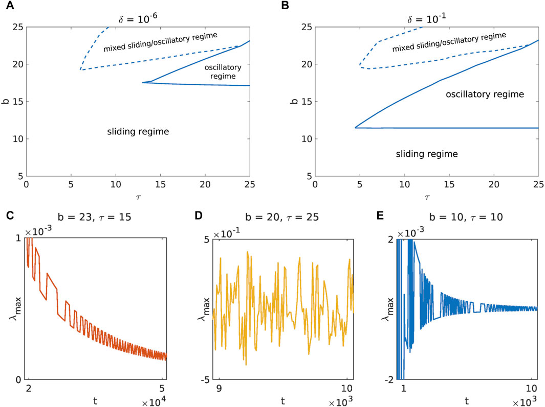
Figure 8. Comparison of the phase diagrams for a = 3.2, c = 4.8, d = 10−4, k = 1, v = 0.1 and with initial conditions near [(A), δ = 10−6] and far [(B), δ = 10−1] from the fixed point. In the mixed regime, the phase diagram “randomly” alternates between the sliding and oscillatory regime for small changes in b and τ. The diagrams (C–E) show the typical behavior of λmax in the mixed, oscillatory and sliding regime, respectively (δ = 10−6).
As for the joint effect of the friction parameter c and the change in initial conditions, the dynamics of the landslide seems to stabilize for initial conditions away from the fixed point. In particular, it can be seen in Figure 9 that in this case the complex oscillatory regime occurs for lower values of c than when the initial conditions are close to the fixed point.
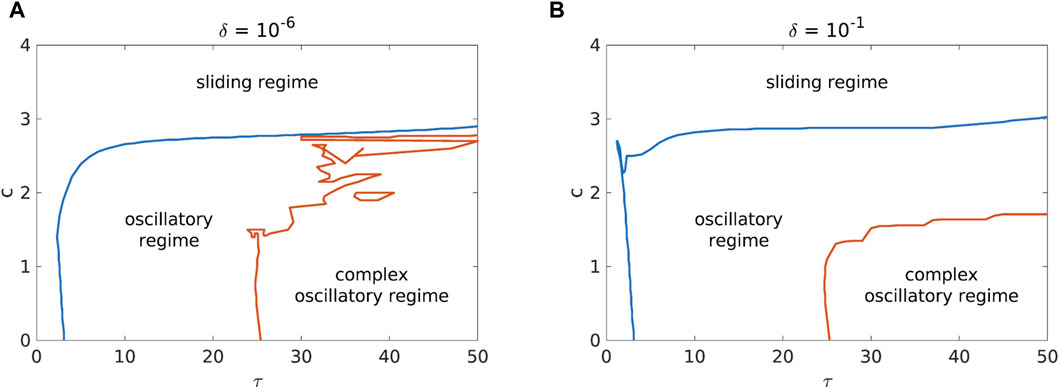
Figure 9. Comparison of the phase diagrams for a = 3.2, b = 7.2, d = 10−4, k = 1, v = 0.1 and with initial conditions near [(A), δ = 10−6] and far [(B), δ = 10−1] from the fixed point.
The interaction of noise and change in initial conditions is shown in Figure 10. It appears that moving away from the fixed point stabilizes the dynamics of the landslide, as complex oscillations only occur for a very narrow range of parameters when δ is away from 0 (Figure 10B).
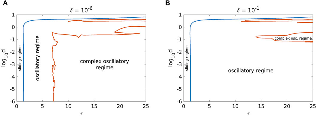
Figure 10. Comparison of the phase diagrams for a = 3.2, b = 7.2, c = 4.8, k = 12, v = 0.1 and with initial conditions near [(A), δ = 10−6] and far [(B), δ = 10−1] from the fixed point.
In this paper we investigate the effects of initial conditions on the dynamics of the phenomenological spring-block model. The initial model is described by a system of stochastic delay differential equations in which both the delay of the displacement and the random background noise are taken into account. By applying the mean-field approximation method, we have formulated a corresponding mean-field variant of the initial model. Such a deterministic mean-field model has qualitatively the same dynamics as the starting stochastic one. The analysis of the changes in the dynamics of the landslide model caused by the varying initial conditions was carried out numerically.
When the initial conditions start near the fixed point, the following dynamical regimes occur: (1) sliding regime, (2) oscillatory regime, (3) complex oscillatory regime, (4) unstable regime, (5) mixed sliding/oscillatory regime. The sliding regime represents the stable equilibrium regime of the creeping landslide. Regular periodic oscillations are considered as the transient unstable regime, while the complex oscillatory regime as well as unstable and mixed sliding regime correspond to the unstable landslide dynamics.
For the initial conditions away from the fixed point, the following can be observed: (1) the change in the initial conditions does not lead to a new dynamical regime, (2) the change in the initial conditions acts as a stabilizing or destabilizing factor, depending on which system parameter it interacts with. The stabilizing effect occurs when interacting with the noise intensity d, the friction parameter c, higher values of the friction parameter a and the spring stiffness (slope deformability) k. This stabilizing effect manifests itself as follows: (1) almost complete suppression of the occurrence of an unstable landslide (interacting with d), (2) partial limitation of the effect of the friction parameters a and c in the sense that an unstable landslide occurs at lower (parameter c) or higher values (parameter a) of the control parameters. A similar effect is captured by the interaction with the spring stiffness (slope deformability) k. The destabilizing effect of changing the initial conditions occurs when interacting with the parameter b and lower values of the parameter a. The destabilizing effect is shown by the fact that a transient oscillatory regime occurs at lower values of the parameter b and the stable sliding regime is completely suppressed at lower values of the parameter a.
As far as the interaction between the displacement delay and the change in the initial conditions is concerned, the change in the initial conditions only has an influence on the effect of the delay if it interacts with the friction parameter b, lower values of the friction parameter a or the noise intensity. In the case of the noise intensity, a change in the initial conditions leads to a complex oscillatory regime that only occurs at higher values of the displacement delay. For the friction parameter b, a change in the initial conditions leads to the appearance of the oscillatory regime for much lower values of the delay, while for the lower values of the parameter a, a change in the initial conditions suppresses the appearance of the stable sliding regime for low values of the time delay.
From an engineering point of view, the results of our research underline the importance of initial conditions for landslide dynamics. The nature of this effect (stabilizing or destabilizing) strongly depends on the friction parameters, the noise intensity, the displacement delay and the deformability of the slope.
In our research, we found that at extremely high values of displacement delay (which are hardly to be expected under real conditions), long-lasting stick-slip-like motion occurs (e.g., τ = 60, k = 6, δ = 10–6, t up to 105), which can be considered as the most representative phenomenological model of real landslide dynamics. Further research should investigate the possible occurrence of these stick-slip dynamics for a much smaller delay, which should bring the results closer to those expected in practice. However, we have observed short-term transient stick-slip behavior for a delay as small as τ = 5 (e.g., τ = 5, k = 10, δ = 10–6, t ≲ 50 and τ = 15, k = 5, δ = 10–6, t ≲ 1000).
The experimental verification of the proposed model and its conclusions could in principle be performed with a similar setup as in Pajalić et al. (2021) or Cheng et al. (2021). To compute the variables of the MF model and observe their evolution over time, a precise and fast mapping of the large number of points on the slope would be required. The initial steady-state velocity of the landslide could be controlled by adjusting the speed of the artificial rain as well as the steepness of the slope. On the other hand, the variation of the friction parameters could be realized by using different soil samples. This could be an interesting topic for future research.
The raw data supporting the conclusion of this article will be made available by the authors, without undue reservation.
DP: data curation, formal analysis, investigation, resources, software, validation, visualization, writing–original draft, writing–review and editing. NT-V: data curation, formal analysis, investigation, supervision, validation, writing–review and editing. NV: formal analysis, methodology, writing–review and editing. SK: conceptualization, project administration, supervision, writing–original draft, writing–review and editing.
The author(s) declare financial support was received for the research, authorship, and/or publication of this article. This research was supported by the Ministry of Science, Technological Development and Innovation, Republic of Serbia through: Grant Agreements with University of Belgrade–Faculty of Pharmacy No. 451-03-47/2023-01/200161 and 451-03-65/2024-03/200161. Grant Agreement with University of Belgrade–Faculty of Mining and Geology No. 451-03-47/2023-01/200126.
The authors declare that the research was conducted in the absence of any commercial or financial relationships that could be construed as a potential conflict of interest.
All claims expressed in this article are solely those of the authors and do not necessarily represent those of their affiliated organizations, or those of the publisher, the editors and the reviewers. Any product that may be evaluated in this article, or claim that may be made by its manufacturer, is not guaranteed or endorsed by the publisher.
The Supplementary Material for this article can be found online at: https://www.frontiersin.org/articles/10.3389/feart.2024.1374942/full#supplementary-material
Chau, K. (1995). Landslides modeled as bifurcations of creeping slopes with nonlinear friction law. Int. J. Solids Struct. 32, 3451–3464. doi:10.1016/0020-7683(94)00317-P
Chau, K. T. (1999). Onset of natural terrain landslides modelled by linear stability analysis of creeping slopes with a two-state variable friction law. Int. J. Numer. Anal. Methods Geomechanics 23, 1835–1855. doi:10.1002/(sici)1096-9853(19991225)23:15<1835::aid-nag2>3.3.co;2-u
Cheng, H., Han, L., Wu, Z., and Zhou, X. (2021). Experimental study on the whole failure process of anti-dip rock slopes subjected to external loading. Bull. Eng. Geol. Environ. 80, 6597–6613. doi:10.1007/s10064-021-02311-5
Davis, R. (1992). Modelling stability and surging in accumulation slides. Eng. Geol. 33, 1–9. doi:10.1016/0013-7952(92)90031-S
Franović, I., Todorović, K., Vasović, N., and Burić, N. (2016). Mean field dynamics of networks of delay-coupled noisy excitable units. AIP Conf. Proc. 1738, 210004. doi:10.1063/1.4951987
Fuentes, M. A., Sato, Y., and Tsallis, C. (2011). Sensitivity to initial conditions, entropy production, and escape rate at the onset of chaos. Phys. Lett. A 375, 2988–2991. doi:10.1016/j.physleta.2011.06.039
Gardiner, W. P. (1997). Statistical Analysis Methods for chemists: a software-based approach. London, United Kingdom: The Royal Society of Chemistry.
Iverson, R., George, D., Allstadt, K., Reid, M., Collins, B., Vallance, J., et al. (2015). Landslide mobility and hazards: implications of the 2014 oso disaster. Earth Planet. Sci. Lett. 412, 197–208. doi:10.1016/j.epsl.2014.12.020
Iverson, R. M., Reid, M. E., Iverson, N. R., LaHusen, R. G., Logan, M., Mann, J. E., et al. (2000). Acute sensitivity of landslide rates to initial soil porosity. Science 290, 513–516. doi:10.1126/science.290.5491.513
Kostić, S., and Stojković, M. (2023). Colored noise in river level oscillations as triggering factor for unstable dynamics in a landslide model with displacement delay. Front. Earth Sci. 11. doi:10.3389/feart.2023.1267225
Kostić, S., Todorović, K., Lazarević, Ž., and Prekrat, D. (2023a). Friction and stiffness dependent dynamics of accumulation landslides with delayed failure. Entropy 25, 1109. doi:10.3390/e25071109
Kostić, S., Vasović, N., Franović, I., Jevremović, D., Mitrinovic, D., and Todorović, K. (2014). Dynamics of landslide model with time delay and periodic parameter perturbations. Commun. Nonlinear Sci. Numer. Simul. 19, 3346–3361. doi:10.1016/j.cnsns.2014.02.012
Kostić, S., Vasović, N., Todorović, K., and Prekrat, D. (2023b). Instability induced by random background noise in a delay model of landslide dynamics. Appl. Sci. 13, 6112. doi:10.3390/app13106112
Lax, M., Cai, W., and Xu, M. (2006). Random processes in physics and finance. Oxford, United Kingdom: Oxford University Press. doi:10.1093/acprof:oso/9780198567769.001.0001
Li, C., Yu, G., Li, L., Yu, H., Fan, Y., Lei, J., et al. (2023). Reliability analysis of seismic slope incorporating interactions among multiple sliding blocks using imbalance thrust force method in primary sliding direction. Sustainability 15, 12350. doi:10.3390/su151612350
Morales, J. E., James, G., and Tonnelier, A. (2017). Traveling waves in a spring-block chain sliding down a slope. Phys. Rev. E 96, 012227. doi:10.1103/PhysRevE.96.012227
Pajalić, S., Peranić, J., Maksimović, S., Čeeh, N., Jagodnik, V., and Arbanas, Å. (2021). Monitoring and data analysis in small-scale landslide physical model. Appl. Sci. 11, 5040. doi:10.3390/app11115040
Qin, S., Jiao, J. J., and Wang, S. (2002). A nonlinear dynamical model of landslide evolution. Geomorphology 43, 77–85. doi:10.1016/S0169-555X(01)00122-2
Schilirò, L., Poueme Djueyep, G., Esposito, C., and Scarascia Mugnozza, G. (2019). The role of initial soil conditions in shallow landslide triggering: insights from physically based approaches. Geofluids 2019, 1–14. doi:10.1155/2019/2453786
Shou, Y., Zhao, X., and Zhou, X. (2022). Novel three-dimensional sarma method with vertical slices for stability analysis of rock slopes. Int. J. Geomechanics 22, 04021302. doi:10.1061/(ASCE)GM.1943-5622.0002275
Vasović, N., Kostić, S., Franović, I., and Todorović, K. (2016). Earthquake nucleation in a stochastic fault model of globally coupled units with interaction delays. Commun. Nonlinear Sci. Numer. Simul. 38, 117–129. doi:10.1016/j.cnsns.2016.02.011
Xu, X., Zhou, X., Huang, X., and Xu, L. (2017). Wedge-failure analysis of the seismic slope using the pseudodynamic method. Int. J. Geomechanics 17, 04017108. doi:10.1061/(ASCE)GM.1943-5622.0001015
Zhang, X., and Zhou, X. (2018). Analysis of the numerical stability of soil slope using virtual-bond general particle dynamics. Eng. Geol. 243, 101–110. doi:10.1016/j.enggeo.2018.06.018
Keywords: slope stability, global dynamics, bifurcation, time delay, friction
Citation: Prekrat D, Todorović-Vasović NK, Vasović N and Kostić S (2024) Complex global dynamics of conditionally stable slopes: effect of initial conditions. Front. Earth Sci. 12:1374942. doi: 10.3389/feart.2024.1374942
Received: 23 January 2024; Accepted: 04 March 2024;
Published: 19 March 2024.
Edited by:
Xiaoping Zhou, Chongqing University, ChinaReviewed by:
Milan Stojkovic, Institute for Artificial Intelligence R&D Serbia, SerbiaCopyright © 2024 Prekrat, Todorović-Vasović, Vasović and Kostić. This is an open-access article distributed under the terms of the Creative Commons Attribution License (CC BY). The use, distribution or reproduction in other forums is permitted, provided the original author(s) and the copyright owner(s) are credited and that the original publication in this journal is cited, in accordance with accepted academic practice. No use, distribution or reproduction is permitted which does not comply with these terms.
*Correspondence: D. Prekrat, ZHJhZ2FuLnByZWtyYXRAcGhhcm1hY3kuYmcuYWMucnM=
Disclaimer: All claims expressed in this article are solely those of the authors and do not necessarily represent those of their affiliated organizations, or those of the publisher, the editors and the reviewers. Any product that may be evaluated in this article or claim that may be made by its manufacturer is not guaranteed or endorsed by the publisher.
Research integrity at Frontiers
Learn more about the work of our research integrity team to safeguard the quality of each article we publish.