 Jolanta Nastula1
 Justyna Śliwińska-Bronowicz
 Małgorzata Wińska
94% of researchers rate our articles as excellent or good
Learn more about the work of our research integrity team to safeguard the quality of each article we publish.
Find out more
ORIGINAL RESEARCH article
Front. Earth Sci., 10 April 2024
Sec. Solid Earth Geophysics
Volume 12 - 2024 | https://doi.org/10.3389/feart.2024.1369106
Mass changes in the hydrosphere represent an important contributor to polar motion (PM) variations, especially at seasonal time scales (i.e., annual and semiannual). Although well studied, hydrological angular momentum (HAM) remains a major source of uncertainty in estimating PM excitation. In this work, we use a large number of climate models from the sixth phase of the Coupled Model Intercomparison Project (CMIP6) to determine HAM series both from individual models and their combination, formed with a multi-model mean, a weighted mean, and a three-cornered hat (TCH) method. The CMIP6-based HAM series are analysed in several spectral bands and evaluated with a reference hydrological signal in geodetically observed PM excitation (GAO). HAM determined from CMIP6 were also compared to HAM calculated from Gravity Recovery and Climate Experiment (GRACE) measurements. We find that while climate models do not allow for reliable estimation of non-seasonal changes in HAM, they can help interpret seasonal variability. For annual prograde and semiannual retrograde oscillations, several combined CMIP6-based series exhibit higher amplitude and phase consistency with GAO than the corresponding series computed from GRACE data. Whether one uses a simple average of the models, a weighted average, or a combination of models from the TCH method has little impact on the resulting HAM series and their level of agreement with GAO. Our study advances the understanding of hydrological signal in Earth’s rotation at seasonal time scales.
The distribution of masses of atmosphere, ocean, terrestrial hydrosphere, and cryosphere is constantly changing. These dynamic processes, combined with movements in the solid part of the Earth, give rise to fluctuations in the Earth’s rotation (Munk and MacDonald, 1960). The changes in the position of the Earth’s rotation axis relative to the surface, known as polar motion (PM), can be represented by two coordinates, xP and yP. By studying PM variations through geodetic observations and geophysical models, we can gain insight into processes and interactions occurring within the Earth system.
The primary contributors to changes in PM are attributed to the atmosphere, including winds and surface pressure (e.g., Barnes et al., 1983; Chao and Au, 1991; Gross et al., 2003), and the oceans, involving ocean bottom pressure and currents (Wahr, 1983; Dickey et al., 1993; Ponte et al., 1998; Gross et al., 2003). Barnes et al. (1983) and Brzeziński (1992) introduced the concept of effective angular momentum (EAM) functions, which consist of two equatorial components (χ1, χ2) and one axial component (χ3), to describe the Earth’s rotation variations. These EAM components have geophysical interpretations and can be derived from models, data or syntheses thereof. The four EAM functions—atmospheric angular momentum (AAM), oceanic angular momentum (OAM), hydrological angular momentum (HAM), and cryospheric angular momentum (CAM)—are contingent on their corresponding physical phenomena affecting PM, specifically, mass transport within the atmosphere, oceans, continental hydrosphere, and cryosphere. While the contributions of AAM and OAM have been widely analysed and are well described in previous studies (Ponte et al., 1998; Gross et al., 2003; Dobslaw et al., 2010; Quinn et al., 2019; Börger et al., 2023), the roles of HAM and CAM remain far from fully understood.
Recent studies on this topic have focused on determining HAM from either measurements of the Earth’s gravity field variations delivered by the Gravity Recovery and Climate Experiment (GRACE) and its follow-on mission (GRACE-FO) (Jin et al., 2010; Cheng et al., 2011; Seoane et al., 2012; Meyrath and van Dam, 2016; Göttl et al., 2019; Nastula et al., 2019) or from global models of the continental hydrosphere (Chen et al., 2000; Chen et al., 2005; Brzeziński et al., 2009; Wińska et al., 2017; Nastula et al., 2019). However, these studies indicate that HAM series derived from various types of data differed noticeably, primarily in terms of the amplitudes of individual oscillations. These papers also showed that of the various oscillations present in HAM, seasonal signals (mainly annual and semi-annual) are the most accurately determined. It has also been shown that compared with the modelled HAM, HAM derived from GRACE/GRACE-FO exhibited higher consistency with the hydrological signal in geodetically observed PM excitation (geodetic residuals, GAO) (Nastula et al., 2019; Śliwińska et al., 2019). However, despite its uniqueness and high measurement accuracy, satellite gravity data have some drawbacks, such as the length of the data record (from 2002 to the present, with a 1-year gap between the end of the GRACE operation and the launch of the GRACE-FO). The relatively short observation period poses challenges in studying long-term changes in PM excitation, such as the influence of decadal climate change effects in Earth’s subsystems on this process (Adhikari and Ivins, 2016).
Free-running climate models, integrated for centuries with natural and anthropogenic forcing, represent an alternative route for determining HAM. Climate models are fundamental for scientists to comprehend historical and potential future climate alterations. These models replicate the complex interplay of atmospheric, terrestrial and oceanic physics, chemistry, and biology (Taylor et al., 2012). A large number of climate models are stored and made publicly available in the frame of the Coupled Model Intercomparison Project (CMIP) (Eyring et al., 2016a). The newest release of this initiative, CMIP Phase 6 (CMIP6), represents a substantial expansion over its previous versions in terms of the number of modelling groups participating in the project, the number of models registered, the number of future scenarios examined, and the number of different experiments conducted (Eyring et al., 2016a; Eyring et al., 2016b; Eyring et al., 2016c). CMIP6 products can be used in many scientific applications, including studying past, present, and future changes in water storage around the world. However, CMIP6 models are subject to the same limitations as hydrological models and represent broadband (i.e., non-seasonal and interannual variability) only in a statistical sense, given the lack of data constraints. Moreover, in contrast to GRACE/GRACE-FO estimates, they do not provide comprehensive information on all terrestrial water storage (TWS) components. In particular, there is a lack of representation of groundwater storage and ice mass changes in the polar regions.
Previous studies have mainly used climate data from CMIP to study past and future climate changes and their impact on various natural, economic, and social factors (Tokarska et al., 2020; Lalande et al., 2021; Cos et al., 2022). Some authors have also utilised climate data to analyse TWS variations over various areas (Freedman et al., 2014; Jensen et al., 2019; Jensen et al., 2020a; Jensen et al., 2020b ; Wu et al., 2021). However, there are hardly any studies that have applied CMIP6-based TWS for deriving HAM. One of the initial endeavours in this direction was our previous work (Nastula et al., 2022), where we examined HAM computed from a number of models derived from CMIP6. The main objective of that study was to check whether the latest climate models provide realistic data to determine HAM. We analysed 99 single CMIP6 historical models. We assessed the quality of the computed CMIP6-based HAM in various spectral bands by comparing them with GAO. We attempted to identify one or more CMIP6 individual models that would be most suitable for HAM analyses. However, it was found that the model choice was ambiguous and dependent on many factors, such as the analysed component of the excitation function, spectral range, or period.
The objective of the current study was to explore whether grouping or combining various climate models can improve the consistency between CMIP6-based HAM and GAO. Combining multiple models is a common practice in climate studies (Freedman et al., 2014; Jensen et al., 2019; Grose et al., 2020; Kim et al., 2020). It is advisable for users of CMIP6 data to utilize an ensemble of models, as there is no single optimal climate model. An ensemble considers the model uncertainty in projections and yields more reliable climate forecasts (Parsons et al., 2021).
We investigated groups of CMIP6 outputs formed using the multi-model mean, the weighted mean of selected models, and the more sophisticated three-cornered hat (TCH) method. We compared combined CMIP6-based HAM series with outputs from GRACE and from the Land Surface Discharge Model (LSDM), which is one of the most reliable hydrological models used in PM excitation analysis (Dill, 2008; Dill et al., 2009; Śliwińska et al., 2020). We focused on analysing the energic seasonal oscillations in HAM. These signals can be more precisely determined from both observations and models compared with non-seasonal changes, which usually have smaller amplitudes and are more challenging to accurately determine with numerical models (Brzeziński et al., 2009).
Research on the influence of the terrestrial hydrosphere on PM excitation is an important issue in modern geodesy. PM coordinates belong to Essential Geodetic Variables (EGVs), which are observed variables fundamental for describing the geodetic properties of the Earth and are essential to maintain geodetic observations (Gross, 2022). EGVs are key for determining the shape of the Earth, its orientation in space, and changes in its gravitational field. They are also crucial in defining and implementing reference systems as well as in precise positioning and navigation. Since the coordinates of PM are an essential ECV characterizing the orientation of the Earth and are subjected to constant disturbances from various phenomena, their continuous monitoring using geodetic measurement techniques, as well as understanding the sources of disturbances in the PM, is one of the key tasks of modern geodesy. It was discovered that the alterations in large-scale global wet and dry patterns in TWS accounts for the decadal changes in PM (Adhikari and Ivins, 2016). Therefore, the historical geodetic measurements of PM could potentially provide insights into the severity, duration, and global extent of wet and dry periods, holding important implications for understanding climate change in the 21st century.
On the one hand, climate models can serve as an additional source of data when interpreting PM changes in the absence of observational data. In particular, CMIP6 data allow for the analysis of future changes in PM. On the other hand, validating climate models based on their comparison with GAO will help identify the most reliable models, which can then be used to study the impact of climate change on PM excitation.
The remainder of this paper is organised as follows: Section 2.1 outlines the data and methods we applied to compute GAO. Section 2.3 contains the description of data and methods used to determine HAM. Detailed explanations of the methods employed for grouping the CMIP6-based data are provided in Section 2.3. Section 3.1 presents a comparison of various HAM series, while Section 3.2 focuses on selecting the most appropriate clustered CMIP6 models for analysing HAM in the seasonal spectral band. Finally, Section 4 summarises the results and provides conclusions.
Geodetic excitation functions of the PM can be determined from the observed pole coordinates (xP, yP) as measured with space geodetic techniques. To derive excitation functions from observed xP and yP values, the Liouville equation (Vicente and Wilson, 2002) can be used to convert xP, yP into equatorial components (χ1, χ2) of geodetic angular momentum (GAM). These GAM components should thus be interpreted as the excitation necessary to change the motion of the Earth’s rotational axis in accordance with observations made by space geodesy. GAM can be compared to EAM functions (sum of AAM, OAM, and HAM) derived from geophysical models of the atmosphere, oceans, and hydrosphere.
Typically, the hydrological signal in GAM can be isolated by removing the contributions of the atmosphere and ocean (e.g., Jin et al., 2010; Nastula et al., 2019) to obtain the GAO. In our previous research (e.g., Wińska et al., 2017; Śliwińska et al., 2019; Nastula et al., 2022), the GAO was estimated by subtracting the sum of AAM and OAM from GAM:
The resulting GAO series mainly reflects the hydrological signals in PM excitation but also solid-Earth-related signals from glacial isostatic adjustment (GIA). Additional residual oceanic signals in GAO arise from (1) barystatic sea level changes due to freshwater transfer into the ocean, and (2) ocean gravitational attraction and loading (“sea level fingerprints,” Adhikari and Ivins, 2016). The impact of such variations on PM excitation can be described with sea-level angular momentum (SLAM) (Dill, 2008). SLAM primarily accounts for the global distribution of hydrological and atmospheric excess mass, which is dispersed into the ocean (Dill and Dobslaw, 2019; Dobslaw and Dill, 2019). Additionally, it encompasses the gravitational impact of loading and self-attraction that influences ocean sea levels. The SLAM series developed by Deutsches GeoForschungsZentrum GFZ are calculated from the global patterns of atmospheric and terrestrial water storage masses, utilizing the sea-level equation (Tamisiea et al., 2010) for calculation. For this purpose, the European Center for Medium–Range Weather Forecasts (ECMWF) model for the mass of the atmosphere and the LSDM model for the mass of the hydrosphere were utilized. SLAM ensures the equilibrium of global mass within the model system, maintaining a constant sum of the total mass across all four distinct EAM components (AAM, OAM, HAM, and SLAM) at any time.
GRACE- and model-based HAM are free of GIA and SLAM signals. For GRACE-based HAM, we eliminated all the signals related to the oceans by applying a zero mask over the ocean areas (see Section 2.2). The post-glacial rebound effect from GRACE data is usually removed by computing centres providing GRACE Level-3 data. An appropriate glacial isostatic adjustment (GIA) model is used for this purpose. Hydrological models only provide information on mass changes over continents, so there is no need to separate GIA or ocean-related signals. While retaining GIA within GAO solely impacts the trends in these series, which are not analysed here, retaining SLAM within GAO could potentially lead to an increased standard deviation of the series. Therefore, in this study, we modified Eq. 1 to additionally remove signals related to the SLAM and GIA from GAO:
AAM, OAM and SLAM data used in this study to compute GAO according to Eq. (2) were provided by Earth System Modelling group at GFZ (ESMGFZ), while GIA model was provided by Peltier et al. (2018). SLAM estimate used for GAO calculation is determined from the ECMWF reanalysis pressure and LSDM mass changes over land. We acknowledge that the comparison between GAO and CMIP6-based HAM might favour those CMIP6 models that exhibit similar atmospheric and hydrological mass changes as the models used by ESMGFZ (ECMWF and LSDM, respectively). Although beyond the scope of this work, calculating SLAM estimates for each CMIP6-based HAM series could improve the consistency between GAO and HAM. It should be recalled that the choice of AAM and OAM models for GAO computation is also important. Utilizing AAM and OAM data from ESMGFZ to calculate GAO yields consistent results with GRACE-based HAM estimations, because both GRACE atmosphere and ocean dealiasing data and ESMGFZ excitation functions are based on the same input models. The LSDM-based HAM series by GFZ maintains the mass balance between all EAM components (AAM, OAM, HAM, SLAM). However, this consistency is not preserved for CMIP6-based HAM. A possible solution would be to use CMIP6 variables for atmospheric pressure, winds, ocean bottom pressure and currents to calculate our EAM functions ourselves. However, not all CMIP6 outputs used in our work have such data. A summary of data used to calculate the GAO series is given in Table 1.
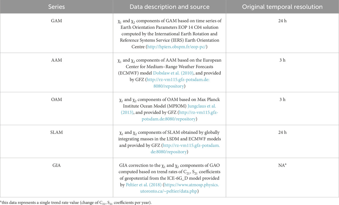
Table 1. Summary of datasets used for GAO computation.
Before computing GAO, all the series were filtered using a Gaussian filter with full width at half maximum (FWHM) equal to 60 days and interpolated into the same time interval (i.e., between January 2003 and January 2014) to maintain consistency with the CMIP6-based and GRACE-based HAM series.
To calculate the equatorial components (χ1, χ2) of the HAM from TWS distribution, we employed the following formulas (as described by Barnes et al., 1983; Eubanks, 1993):
where
To determine TWS from CMIP6 outputs, we utilised two variables: snow water equivalent, representing the equivalent amount of liquid water stored in the snow cover, and soil water storage, which includes water in all phases for all soil layers. By summing up these two variables, we obtained CMIP6-based TWS.
It should be kept in mind that the CMIP6 models are not homogeneous in terms of spatial and temporal resolution, the period for which data are available, and the number of files for each variable. Therefore, the input CMIP6 variables require preselection. For the purpose of this study, multiple files for a single variable at different time intervals were merged into a single extended output. We focused on the period between 2003 and 2014, excluding any models for which there was incomplete data coverage during this period. This resulted in the inclusion of 99 TWS fields from historical CMIP6 models with varying spatial resolutions, which were then interpolated into regular 1° grids.
As a comparative dataset, we used TWS from the GRACE Level-3 release-6 (RL06) solution provided by the Center for Space Research (CSR). The CSR RL06 solution has been shown to have the highest consistency between HAM and GAO at seasonal and non-seasonal time scales (Śliwińska et al., 2021). Level-3 data processing at CSR involved filtering with a 300-km Gaussian filter and implementing various corrections. These include removing the non-tidal atmospheric and oceanic impacts through the use of atmosphere and ocean dealiasing (AOD) data, considering the effects of post-glacial rebound by implementing a GIA model, replacement of the C20 spherical harmonic (SH) coefficient with the more accurate estimate provided by the satellite laser ranging (SLR) technique, the addition of degree-1 SH coefficients (not measured by GRACE), and truncation of SH coefficients at degree 60 (Bettadpur, 2018). It is important to mention that GRACE-based TWS grids contain data for both land and ocean areas. To focus only on data from continents, we utilised GRACE-based grids of TWS anomalies with a mask over the oceans to eliminate all oceanic signals. This operation was not needed when applying the climate models because the CMIP6-based variables used in this study include information for continental areas only.
In addition, we compared the CMIP6- and GRACE-based HAM series with HAM computed from LSDM and delivered by GFZ (Dill, 2008; Dill et al., 2009; data are available at the GFZ website: http://rz-vm115.gfz-potsdam.de:8080/repository). The HAM series derived from LSDM reflects the impact of not only soil moisture and snow water on PM excitation but also surface water (rivers, lakes, and wetlands), shallow groundwater, and water flows in rivers and aquifers (Dobslaw et al., 2010). We have previously shown (Śliwińska et al., 2020) that LSDM-based HAM can capture the amplitudes of annual oscillations in the GAO very well.
Through the application of Eqs 3, 4, we obtained 99 time series of χ1 and χ2 components of the CMIP6-based HAM. The common practice in climate research is to study ensembles of models rather than their individual realisations (Jensen et al., 2020b; Grose et al., 2020). In this study, we adhered to the standard practice by examining representations of various ensembles of CMIP6-based HAM. We considered two methods of forming groups of models, based on which the combined series were determined (see details in Table 2):
1. Creating groups according to the institutes that developed the models which were then named after the names of the institutes, i.e., ACCESS, BCC, CanESM5, GISS, MIROC, MPI, and MRI;
2. Assigning all the 99 CMIP6-based HAM series to one group referred to as ALL.
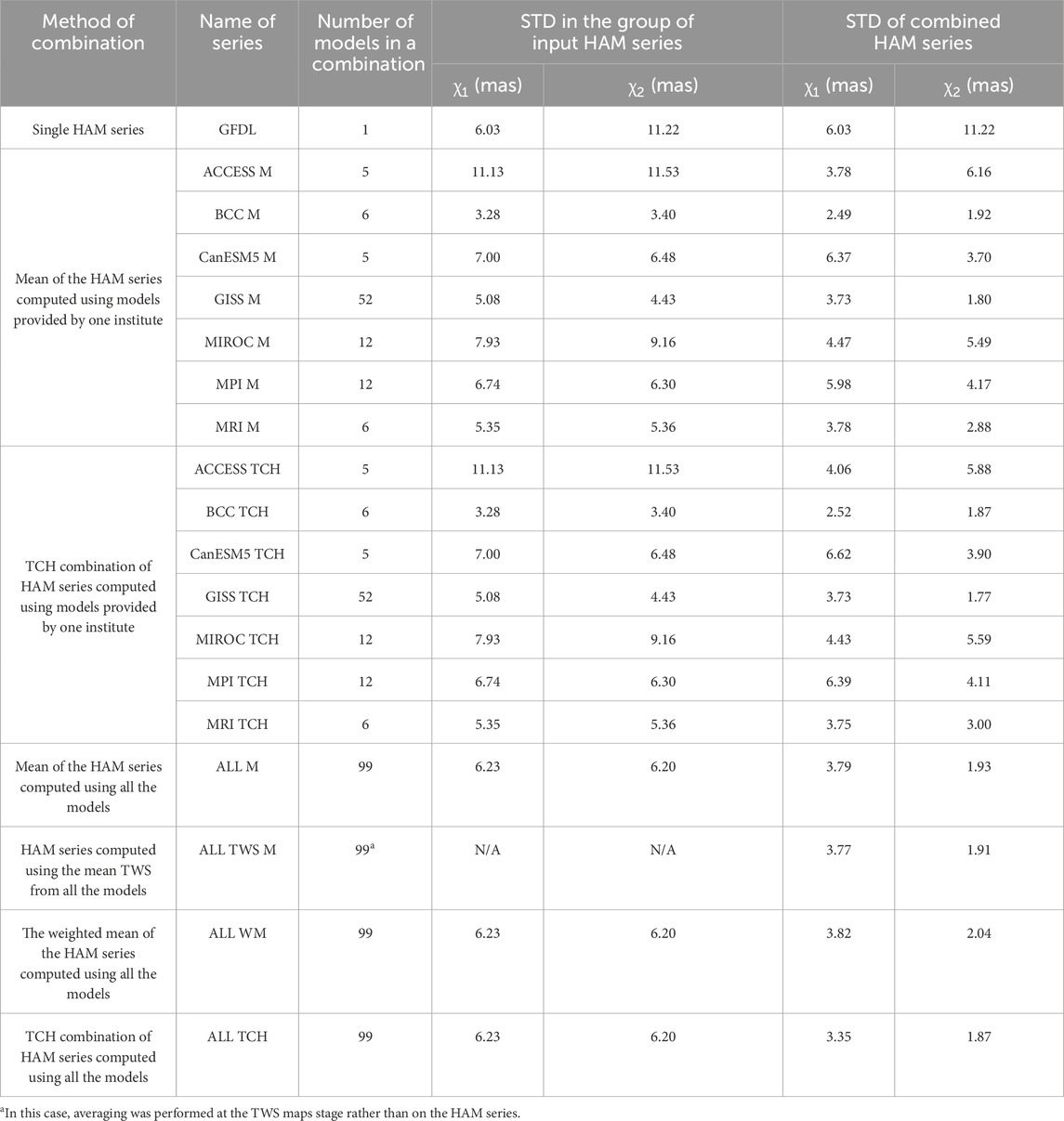
Table 2. List of combined HAM series used in the analyses, number of single models used for combination, values of STD in the group of the input HAM series, and STD of the combined HAM series. The STD values were computed after removing trends.
The HAM series determined based on the GFDL model constitute a distinct category because only one model from the GFDL group contained data for the entire 2003–2014 period.
First, for each group of CMIP6-based HAM series formed according to institute, we calculated the mean of the series from a given institute (M). We then applied the TCH method to develop more complex combinations within groups of institutes. The TCH method enables an estimate of the variance of the individual noise in each series while considering specific assumptions about the correlations between these internal noises. Here, we applied a generalised TCH method, which does not assume zero correlation between the tested series, following the work of Börger et al. (2023), Koot et al. (2006) and Quinn et al. (2019). In general, exploiting the TCH method in combining series reduces the noise within the HAM series (Śliwińska et al., 2022). The detailed description of the TCH method together with relevant equations are given in the Supplementary Material.
We then calculated the combined HAM from all 99 analysed CMIP6 models using the mean and TCH method (ALL M and ALL TCH). In addition, we included the weighted average of HAM computed from all 99 models (ALL WM as a weighted mean of 99 single CMIP6-based series). The weights were computed as the inverse of the squared standard deviation of differences between GAO and the CMIP6-based HAM series.
It is worth noting that our averaging was performed at the level of the HAM series, which means that we first determined the HAM series based on TWS maps from individual models. Then, we calculated the combined HAM based on a single HAM series. To check the potential impact of the stage of averaging within the process on the combined HAM obtained, we also performed averaging one step earlier (at the TWS maps stage) and before calculating HAM. To achieve this, we first computed the average TWS map from the 99 CMIP6-based TWS maps and consequently determined a single combined HAM series–ALL TWS M.
In total, we obtained 19 HAM series and the groups of CMIP6 models formed according to the providing institute are not equal in number (see Table 2). The GISS group contains the largest number of members (52 single models), whereas CanESM5 and ACCESS have five members each. The application of the criteria established during pre-selection resulted in only one model in the GFDL group.
The method of combining series does not have a noticeable impact on the STD of each series as mean HAM computed using the average of models from one institute and the corresponding combined HAM obtained from the TCH method (e.g., BCC M and BCC TCH) have similar STD values (Table 2). The stage at which the results are averaged also has no visible impact on the combined result because the ALL M and ALL TWS M series have almost identical STD values. Comparing the STD values among the groups shows that the most diverse group of models is ACCESS (STD in the group is equal to 11.13 and 11.53 mas for χ1 and χ2, respectively), despite this group being one of the smallest (consisting of only five individual models). In turn, GISS M models, which make up a group of 52 models, are highly similar to each other (STD in the group is equal to 5.08 and 4.43 mas for χ1 and χ2, respectively). Comparison of the STD of the resulting combined HAM series proves that in the case of χ1, the highest STD is observed for CanESM5 M, CanESM5 TCH, and MPI TCH (STD higher than six mas), while for χ2, the highest STD is for ACCESS M (STD above six mas).
Figure 1 shows the time series of all combined CMIP6-based HAM series analysed in this study, together with the range between minimum and maximum, which was determined on the basis of the input series used for the combination. Specifically, Figures 1A–N depict series grouped according to the providing institute determined either as a simple mean or as a combination from the TCH method. In Figures 1O, P, we present a comparison of combined HAM series derived from all individual CMIP6 models using four methods (simple mean (ALL M), weighted mean (ALL WM), TCH (ALL TCH), and HAM from mean TWS (ALL TWS M)). Furthermore, Figures 1Q, R include a standalone HAM series obtained from a single GFDL model.
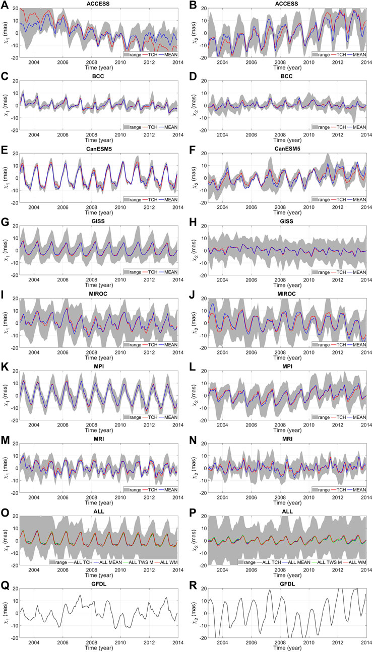
Figure 1. The χ1 (left) and χ2 (right) components of the HAM series: mean and combined HAM series computed for each group designated according to the providing institute (A–N), mean and combined HAM series computed from all single 99 models (O, P), and HAM series computed from the single GFDL model (Q, R). Each combined series was contrasted with the range between minimum and maximum, which was determined on the basis of the input series used for the combination.
Figure 1 demonstrates that the spread of results relative to the mean value does not seem to depend on the number of members in the model groups and is most pronounced for the MIROC, ACCESS, and GISS ensembles. It is also evident that both the calculation of the average and the combination of models using the TCH method yield a similar pattern for the determined series, except for ACCESS-based HAM, where both methods result in differences in the trend. Interestingly, in the case of MPI and CanESM5, there is a greater spread of results relative to the mean for the χ2component compared with the χ1component. Series computed as combinations from all models provided by all institutes are characterised by small amplitudes, which is likely to be because HAM series from all 99 models were averaged and thus the resulting combined series are relatively flat.
In this section, we analyse all CMIP6-based HAM series and compare them with GAO, GRACE-based HAM, and LSDM-based HAM. Figure 2 shows the amplitude spectra of all HAM series and the GAO series. These spectra provide insights into the distribution of amplitudes of particular oscillations in both prograde (counter-clockwise) and retrograde (clockwise) components of the series. To obtain these spectra, the Fourier transform band pass filter (FTBPF) method (Kosek, 1995) was applied to complex components (χ1+iχ2) of the HAM and GAO series. The spectra are dominated by the annual oscillation (Figure 2). Applying the average and the advanced TCH combination method to the HAM series obtained from CMIP6 yields nearly identical results. Some variations in amplitudes can be observed among spectra obtained from the various CMIP6 inputs. The annual oscillation in GAO (both for the prograde and retrograde terms) generally has a larger amplitude than the CMIP6-based series. It should be noted that in the spectra obtained from GAO, GRACE, and LSDM data, the annual retrograde component predominates over the prograde annual component; however, the opposite relationship is observed in the case of spectra obtained from CMIP6 data: the annual prograde component has larger amplitudes than the annual retrograde component. For the semiannual oscillations, the amplitudes of the prograde term for all HAM series are smaller than those of the GAO series. In the case of the semiannual retrograde part, the oscillation peak for GAO is shifted relative to all of the other series. In the spectra obtained from climate models, a very weak terannual oscillation is also observed.
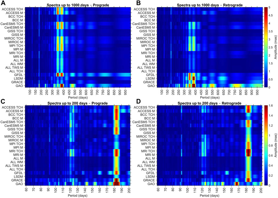
Figure 2. Spectra of complex components (χ1+iχ2) of GAO and HAM computed from GRACE, LSDM, and grouped CMIP6 models: for prograde term computed in a broadband with a 60–1000-day cut-off (A), for retrograde term computed in a broadband with a 60–1000-day cut-off (B), for prograde term computed in a broadband with a 60–200-day cut-off (C), and for retrograde term computed in a broadband with a 60–200-day cut-off (D).
We next compare HAM series in seasonal and non-seasonal spectral bands. The time series of seasonal variations, comprising a combination of annual, semiannual, and terannual oscillations obtained through least-squares fitting to the detrended series, are shown in Figure 3. All the considered series contain seasonal signals with the smallest amplitudes in the case of HAM computed from the BCC and MRI models (Figure 3). The variability of the seasonal oscillation is smaller in the χ2 component than in the χ1 component for HAM obtained from GISS, CanESM5, MPI, and ALL. In contrast, the opposite situation is apparent for seasonal changes observed in GAO, GRACE, LSDM, and GFDL (i.e., the amplitudes of seasonal oscillations are higher for χ2 than for χ1). This is consistent with the results of our previous work, which focused on the HAM analysis (Śliwińska et al., 2020; Śliwińska et al., 2021; Śliwińska et al., 2022).
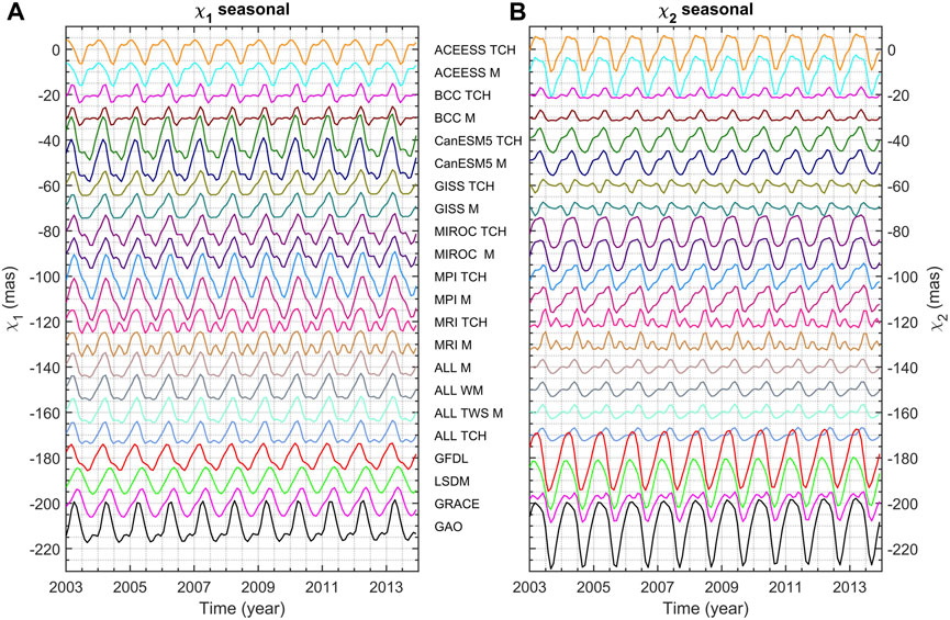
Figure 3. χ1 (A) and χ2 (B) components of seasonal oscillation in GAO and HAM computed from GRACE, LSDM, and grouped CMIP6 models. For better visibility, the series are shifted relative to each other by adding a bias of 10 mas.
The non-seasonal variations, computed by removing seasonal oscillations from the detrended series, were further separated into oscillations with periods longer and shorter than 720 days (Figures 4, 5, respectively). Figures 4, 5 show that averaging and combining HAM series obtained from CMIP6 lead to a notable reduction in amplitudes within the non-seasonal range compared with the variability observed for the GAO, GRACE, LSDM, and GFDL series. All CMIP6-based HAM series, except those computed from GFDL, do not show long-term variability as the plots are almost flat (Figure 4). Notably, for long-term non-seasonal changes, GAO, LSDM-based HAM, and GRACE-based HAM agree well with each other in terms of both amplitudes and phases. At the same time, GFDL-based series are characterised by similar amplitudes to those determined for GAO, LSDM, and GRACE; however, there is a noticeable difference in phase (Figure 4). The amplitudes of other CMIP6-based series are clearly lower than those of GRACE-, LSDM-, and GFDL-based HAM series, as well as GAO. It is apparent that for non-seasonal short-term variation, amplitudes of GAO are much higher than for other series, especially in χ2 component (Figure 5). While GRACE and LSDM data show some variability in this spectral range, the CMIP6 combined series are almost flat. The strongest signal in GAO for non-seasonal short-term variation appears to be for periods of approximately 470 days in prograde and 550 days in retrograde band (Figure 2). These signals are not visible for CMIP6- and LSDM-based series, so we suspect that this may be an effect not modeled by CMIP6 and LSDM, such as groundwater variation (CMIP6 models do not provide information on groundwater, while LSDM only takes into account shallow groundwater), or changes in ice mass (CMIP6 models do not provide such data, while LSDM includes only the annual snow accumulation and melting, with the long-term ice mass kept constant). However, it is known that groundwater and ice mass changes would affect PM at longer time scales (Youm et al., 2017). It might be possible that the variability in GAO observed in Figure 5 is induced by distribution of water between land and ocean or redistribution of water within land. On the other hand, however, the mentioned 470- and 550-day oscillation does not appear in the GRACE data either. Attention should be paid to different time resolution of series: CMIP6 and GRACE data have a monthly resolution, GAM and SLAM used for GAO determination and LSDM are available with a 1-day resolution, AAM and OAM have time resolution of 3 h. However, for consistency between GAO, CMIP6, GRACE and LSDM, all the series were filtered using a Gaussian filter with full width at half maximum (FWHM) equal to 60 days and interpolated into the same time interval. Nonetheless, it can be assumed that the amplitudes of sub-seasonal oscillations may be stronger in GAO than in the other series.
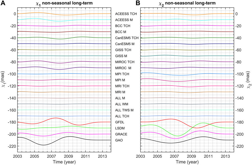
Figure 4. χ1 (A) and χ2 (B) components of non-seasonal long-term variations (with periods longer than 720 days) in GAO and HAM computed from GRACE, LSDM, and grouped CMIP6 models. For better visibility, the series are shifted relative to each other by adding a bias of 10 mas.
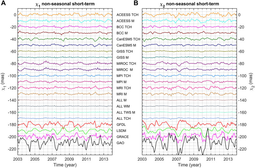
Figure 5. χ1 (A) and χ2 (B) components of non-seasonal short-term variations (with periods shorter than 720 days) in GAO and HAM computed from GRACE, LSDM, and grouped CMIP6 models. For better visibility, the series are shifted relative to each other by adding a bias of 10 mas.
It should be also noted that free-running climate models are not data-constrained climate reanalyses with realistic time tags. Coupled simulations within the CMIP6 initiated from preindustrial states and spanning the entire historical timeline to the contemporary era, are forced with changing solar radiation, aerosols, CO2 concentrations, and land use patterns. Consequently, these experiments are anticipated to replicate climate variability solely in a statistical manner. They may depict the trends and the radiation-forced seasonal variability, but any broadband variability, such as synoptic weather patterns, is purely statistical. In this context, each CMIP6 model has its own random non-seasonal variability and is unlikely to have a common signal for all model runs. Thus, most CMIP6 combinations in the non-seasonal range are close to zero. Therefore, only seasonal variability and trends can be realistically reflected by averages or combinations of climate models.
The time series plots (Figures 3–5) are supplemented with diagrams showing the STD of the series for each oscillation (Figure 6). The STD values of all HAM series and each oscillation are also given in Supplementary Table S1 in the Supplementary Material. The STD values confirm the key finding from the time series analysis that GAO and HAM computed from LSDM, GRACE, and GFDL are characterised by much higher variability than the series of combined CMIP6-based HAM. This is the case for non-seasonal long-term and short-term variations (for both χ1 and χ2) and for seasonal oscillations (for χ2). The combined CMIP6-based HAM is able to accurately capture the amplitudes of oscillations observed for GAO in the case of the χ1 component of seasonal oscillation only.
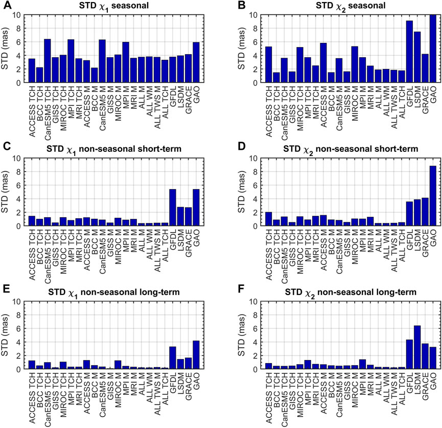
Figure 6. Standard deviation of χ1 and χ2 components of GAO and HAM computed from GRACE, LSDM, and CMIP6 models for seasonal (A, B), non-seasonal short-term (C, D) and non-seasonal long-term (E, F) oscillations.
To check the consistency between GAO and various HAM estimates in different spectral bands, we plot the correlation coefficients (Corr, Figure 7) and normalized root mean square errors (NRMSE, Figure 8) for seasonal, non-seasonal short-term, and non-seasonal long-term variations. NRMSE was calculated by dividing the RMSE of a given series by its STD. The Corr and NRMSE values for all HAM series and each oscillation are also given in the Supplementary Material (Supplementary Table S2 and Supplementary Table S3, respectively). The plots reiterate the good agreement between HAM and GAO at seasonal time scale. For seasonal variations, only two series for χ1 and four series for χ2 exhibit low or negative correlations with GAO, whereas for both short-term and long-term non-seasonal changes, there are noticeably fewer well-performing models.
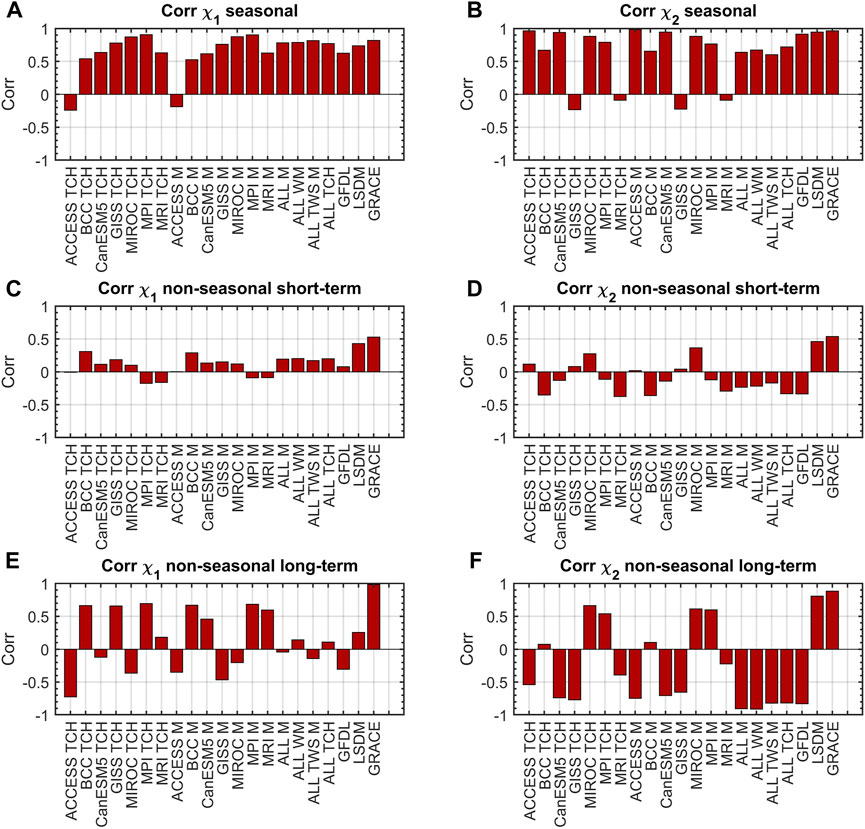
Figure 7. Correlation coefficients (Corr) between GAO and HAM computed from GRACE, LSDM, and CMIP6 models for seasonal (A, B), non-seasonal short-term (C, D) and non-seasonal long-term (E, F) oscillations.
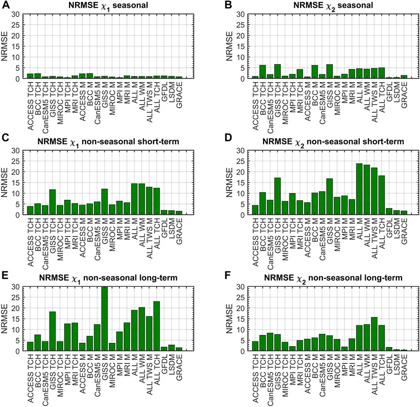
Figure 8. Normalized root mean square error (NRMSE) of HAM computed from GRACE, LSDM, and CMIP6 models for seasonal (A, B), non-seasonal short-term (C, D) and non-seasonal long-term (E, F) oscillations.
It has been demonstrated that the seasonal oscillation (mainly annual) is the most energetic feature in PM excitation (Gross, 2015). Moreover, studies have indicated that HAM has its greatest impact on PM at this time scale (Gross et al., 2003; Brzeziński et al., 2009; Dobslaw et al., 2010; Gross, 2015). The analyses from Section 3.1 confirmed this observation, as we observed highest amplitudes and STD of series, as well as highest agreement between HAM and GAO for seasonal variation. Therefore, in this section, we will focus on this spectral band in more detail. Given the noticeably small amplitude of the terannual oscillation, we decided to investigate the compatibility between CMIP6-based HAM and GAO for annual and semiannual oscillations only. To determine the most reliable model for HAM analysis, we searched for HAM derived from a combined CMIP6 model that had the smallest difference in either amplitude or phase compared with GAO for annual and semiannual oscillation.
Figure 9 presents the absolute values of differences in amplitude of annual oscillation between GAO and all HAM series ordered from lowest to highest value for prograde and retrograde terms separately. In parallel, Figure 10 shows phase differences. The plots also include differences calculated for HAM derived from GRACE and LSDM. Supplementary Tables S4, S5 in the Supplementary Material contain the exact values of these differences. Higher amplitude agreement between HAM and GAO is generally observed for the prograde compared with the retrograde term (Figure 10). In the case of annual prograde oscillation, the highest amplitude correspondence with GAO is obtained for the HAM derived from ACCESS M, GFDL, CanESM5 TCH, CanESM5 M, and ACCESS TCH (differences in amplitude with respect to GAO are below one mas). For annual retrograde oscillation, the smallest amplitude difference is achieved in the LSDM-based series (1 mas). Among the different CMIP6-based series, those calculated based on the GFDL model were the most consistent with the GAO regarding the annual retrograde amplitudes. However, the difference obtained for GFDL is more than one mas greater than that obtained for LSDM. The only series with relatively low values of differences for both prograde and retrograde amplitudes are derived from GFDL, MPI TCH, and MPI M (below two mas for the prograde and below five mas for the retrograde term). It is puzzling that some series, for which the lowest differences in prograde amplitude were obtained, yielded some of the highest differences in retrograde amplitude values (ACCESS M and ACCESS TCH). Notably, while GRACE and LSDM provide the highest amplitude agreement with GAO for the annual retrograde term, for the annual prograde term they exhibit relatively poor agreement.
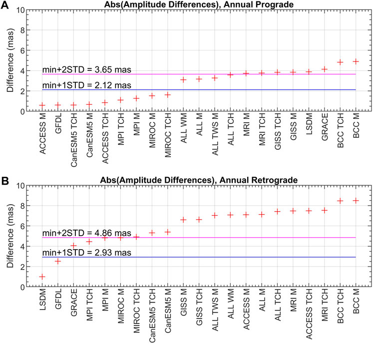
Figure 9. Absolute values of differences in amplitudes of annual prograde (A) and annual retrograde (B) oscillation between GAO and HAM computed from combined CMIP6 models, GRACE, and LSDM. The horizontal blue line shows the value of the smallest amplitude difference with the STDdifferences value added (min+1STDdifferences). The horizontal magenta line presents the value of the smallest amplitude difference with the doubled STDdifferences value added (min+2STDdifferences).
The values of differences with respect to GAO obtained from the amplitude criterion for the annual prograde part do not differ noticeably from each other (Figure 9). To map more clearly the results obtained for individual models, we calculate standard deviation of differences (STDdifferences) with respect to GAO for all HAM series (i.e., STD of the values presented in Figure 9 and Supplementary Table S4 in the Supplementary Material).
For amplitudes of the annual prograde term, STDdifferences was 1.49 mas, whereas for amplitudes of the annual retrograde term, STDdifferences was 1.88 mas. Figure 9 additionally contains the smallest amplitude difference with STDdifferences added (min+1STDdifferences, blue line) and the value of the smallest amplitude difference with the doubled STDdifferences added (min+2STDdifferences, magenta line). From a statistical point of view, the nine series give the same result as the amplitude differences for these series are below the value of min+1STDdifferences. For the three other series, the corresponding values are between min+1STDdifferences and min+2STDdifferences. In turn, for amplitudes of annual retrograde oscillation, the spread of amplitude differences is substantial as the obtained difference is below min+1STDdifferences for just two of the studied series (LSDM and GFDL).
In terms of phases of annual variation, the spread of results is visibly higher for the retrograde than for the prograde term (Figure 10). The highest agreement with GAO for annual prograde variation is observed for CanESM5 M, CanESM5 TCH, BCC M, and BCC TCH (difference below 20°). LSDM- and GRACE-based HAM provide almost the perfect phase match to GAO for the retrograde term (difference below 1°). Among the CMIP6-based HAM series, those based on MPI M, MIROC M, and MIROC TCH give the smallest phase deviations with respect to GAO (below 10°). Notably, while GRACE- and LSDM-based series are in almost perfect phase agreement with GAO for the annual retrograde term, they exhibit much higher differences for the annual prograde term (40° for GRACE and 32° for LSDM).
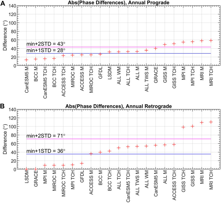
Figure 10. Absolute values of differences in phases of annual prograde (A) and annual retrograde (B) oscillation between GAO and HAM computed from combined CMIP6 models, GRACE, and LSDM. The horizontal blue line shows the value of the smallest amplitude difference with the STDdifferences value added (min+1STDdifferences). The horizontal magenta line presents the value of the smallest amplitude difference with the doubled STDdifferences value added (min+2STDdifferences).
Analysis of the spread of the results for the phases of the annual prograde term shows that the STDdifferences value is as high as 15°, indicating that for nine series, the values of difference with respect to GAO are below min+1STDdifferences. The value of STDdifferences for the phases of the annual retrograde term is equal to 35°. Seven HAM series present statistically the same level of agreement with GAO (differences below min+1STDdifferences), while ten other series present the differences between min+1STDdifferences and min+2STDdifferences. Notably, phase differences for four of the studied 21 series (GISS TCH, GISS M, MRI M, and MRI TCH) exceed 90°.
Figures 11, 12 present absolute values of differences between GAO and HAM series for amplitudes (Figure 11) and phases (Figure 12) of the semiannual oscillation. The corresponding exact values of differences are given in Supplementary Table S6 (amplitudes of semiannual oscillation) and Supplementary Table S7 (phases of semiannual oscillation). The best match for the amplitude is obtained with the HAM determined from GRACE for the semiannual prograde and from BCC M for the semiannual retrograde term (Figure 11). However, from the statistical point of view, as many as eight series for the prograde term and eleven series for the retrograde term present the same level of agreement with GAO (the differences for these series are below min+1STDdifferences). Differences for almost all other series are below min+2STDdifferences. This indicates that only a few series are characterised by noticeably higher amplitude differences. The HAM series that exhibit high amplitude agreement with GAO for both prograde and retrograde terms are those computed from BCC M, BCC TCH, GISS M, and GISS TCH.
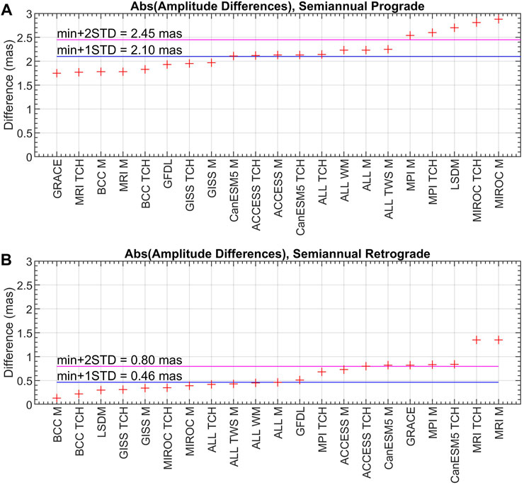
Figure 11. Absolute values of differences in amplitudes of semiannual prograde (A) and semiannual retrograde (B) oscillation between GAO and HAM computed from combined CMIP6 models, GRACE, and LSDM. The horizontal blue line shows the value of the smallest amplitude difference with the STDdifferences value added (min+1STDdifferences). The horizontal magenta line presents the value of the smallest amplitude difference with the doubled STDdifferences value added (min+2STDdifferences).
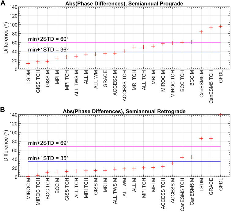
Figure 12. Absolute values of differences in phases of semiannual prograde (A) and semiannual retrograde (B) oscillation between GAO and HAM computed from combined CMIP6 models, GRACE, and LSDM. The horizontal blue line shows the value of the smallest amplitude difference with the STDdifferences value added (min+1STDdifferences). The horizontal magenta line presents the value of the smallest amplitude difference with the doubled STDdifferences value added (min+2STDdifferences).
In terms of phases of semiannual prograde term, three series (LSDM, GISS TCH, and GISS M) present the highest agreement with GAO with difference below 20°. However, statistically, seven other series present a similar level of agreement with GAO since the differences obtained for these series are below min+1STDdifferences. The corresponding differences exceed 80° for only three series. When considering the semiannual retrograde term, almost all series (16 out of 21), had differences with respect to GAO that were below min+1STDdifferences (Figure 12). A phase difference of less than 1° was obtained for MPI the MIROC M series.
In total, we selected eight CMIP6 models that provided the highest agreement between HAM and GAO for the annual and semi-annual oscillation and compared them with the results obtained for GRACE and LSDM. To allow further comparison, we generated four phasor diagrams to show amplitudes and phases of annual prograde and retrograde oscillation for GAO, GRACE-, and LSDM-based HAM as well as HAM computed from two best GAO-fitted CMIP6 models–the first with smallest difference in amplitude and the second with lowest phase difference (Figure 13). Phasor diagrams are an alternative to classical time series representation of seasonal oscillations (Gross et al., 2003; Brzeziński et al., 2005). The length of each vector on a phasor diagram represents the magnitude of amplitude, while the vector direction shows a phase. The reference date used to calculate the phase is 1 January 2003.
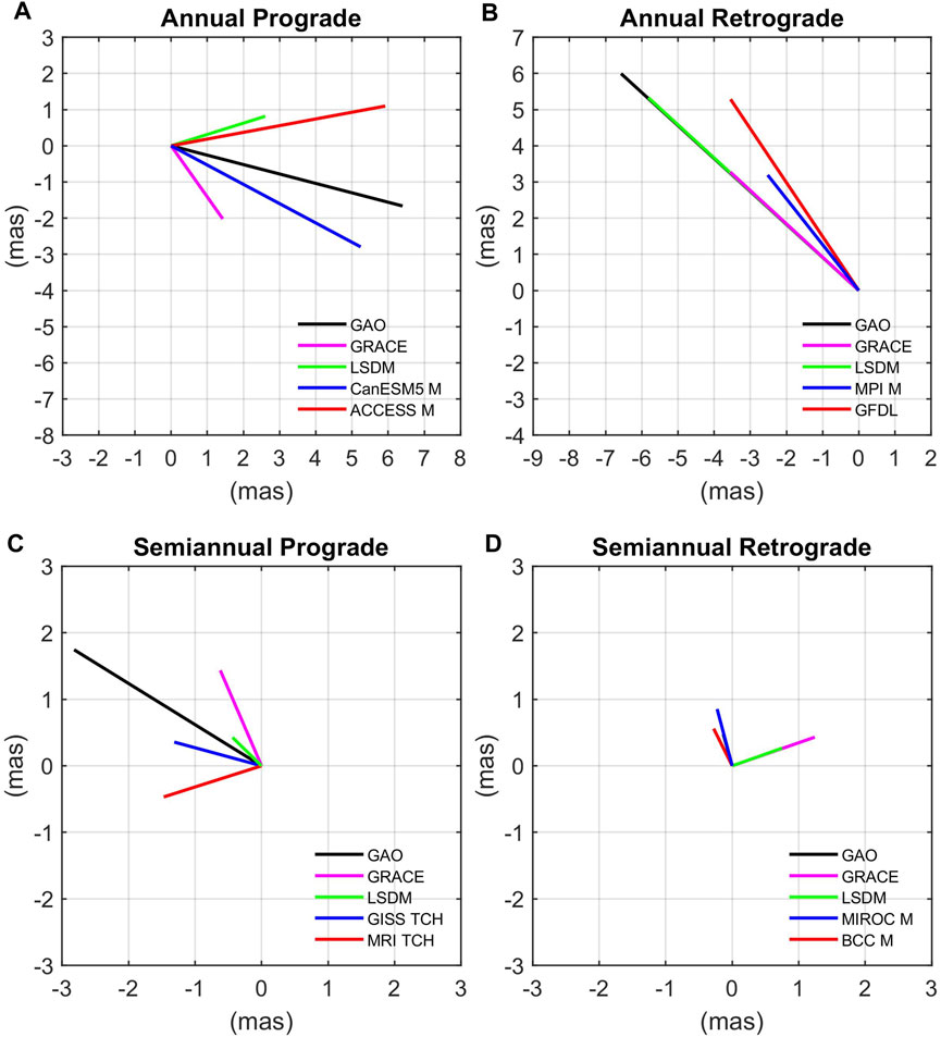
Figure 13. Phasor diagrams of annual prograde (A), annual retrograde (B), semiannual prograde (C), and semiannual retrograde (D) oscillation in GAO and HAM computed from GRACE, LSDM, and the best CMIP6 models chosen for amplitude (red line) and phase (blue line). Reference date for phase is 1 January 2003.
In terms of phases of annual oscillation, the chosen CMIP6 perform better than GRACE and LSDM for the prograde term (CanESM5 M series) and worse than GRACE and LSDM for the retrograde term (MPI M series) (Figures 13A, B). GRACE- and LSDM-based series present a similar level of phase agreement with GAO for the retrograde term (for both series differences with respect to GAO are below 1°). In terms of the amplitudes of annual prograde oscillation, the chosen CMIP6 model (ACCESS M) provides differences with respect to GAO that are lower than LSDM and GRACE. In the case of amplitudes of annual retrograde term, the chosen CMIP6 model (GFDL) gives differences higher than those obtained for LSDM but lower than those obtained for GRACE. For both prograde and retrograde term of annual oscillation, all the HAM series underestimate amplitudes observed for GAO.
The phasor diagrams of semiannual oscillation (Figures 13C, D) show that LSDM- and GRACE-based HAM, as well as the chosen CMIP6-based series, underestimate amplitudes observed for GAO for the prograde term but overestimate GAO amplitudes for the retrograde term. For amplitudes of semiannual prograde oscillation, the chosen CMIP6-based HAM series (MRI TCH) provides amplitude correspondence with GAO at a level similar to GRACE and better than that obtained for LSDM. In turn, for the amplitudes of semiannual retrograde oscillation, the chosen CMIP6 model (BCC M) gives the lowest amplitude differences of all considered series. The best CMIP6-based series for the phase of semiannual prograde term (GISS TCH) presents a lower level of correspondence with GAO than LSDM and higher correspondence than GRACE-based series. For semiannual retrograde variation, the chosen CMIP6 model (MIROC M) provides an almost perfect phase match to GAO, whereas both GRACE- and LSDM-based series are out of phase with GAO by almost 90°.
In general, although in many cases the combined CMIP6-based HAM series provide higher agreement with the GAO than the LSDM- and GRACE-based HAM series (e.g., for the amplitudes and phases of annual prograde oscillation, and amplitudes and phases of semiannual retrograde oscillation), it is not possible to identify a single series that would provide a high correspondence with GAO across all criteria applied.
In this research, we examined the potential enhancement in the agreement between CMIP6-based HAM and GAO by grouping and combining climate models. We examined various combinations of CMIP6-based HAM determined based on classical ensemble mean, weighted mean, and TCH combination. The combinations were determined on the basis of various groups of models, including either only models provided by one institute or all models meeting the selection criteria established at the beginning.
This study confirms the conclusions of our previous work (Nastula et al., 2022) that most of the analysed climate models do not allow for reliable estimation of non-seasonal changes in HAM but can be used to interpret seasonal oscillations in HAM. Therefore, in this study, we focused on annual and semiannual signals in HAM and analysed the amplitude and phase correspondence between CMIP6-based HAM and GAO. We find that the combination of CMIP6 models does not lead to a noticeable improvement in the agreement between HAM and GAO. Moreover, determining the most suitable group of CMIP6 models for studying HAM depends on which oscillation is analysed and whether the analysis considers the amplitude or the phase match with GAO.
We show that, for annual oscillation, the following CMIP6 models exhibit the highest agreement between HAM and GAO: ACCESS M (for amplitude of annual prograde oscillation), GFDL (for amplitude of annual retrograde oscillation), CanESM5 M (for phase of annual prograde oscillation), and MPI M (for phase of annual retrograde oscillation). For semiannual variations, the following models provide the most satisfactory results: MRI TCH (for amplitude of semiannual prograde oscillation), BCC M (for amplitude of semiannual retrograde oscillation), GISS TCH (for phase of semiannual prograde oscillation), MIROC M (for phase of semiannual retrograde oscillation). However, the differences in results between individual models were often very small, thus a better option would be to distinguish a certain group of best-performing models.
A single CMIP6-based HAM cannot meet all the aforementioned criteria, regardless of whether we refer to a single model or a combination of several models. Therefore, additional criteria that integrate both amplitude and phase correspondence should be considered. The problem with attempting to select an optimal group of CMIP6 models for HAM analysis is that often those CMIP6-based series that provide the highest GAO agreement for one criterion exhibit one of the lowest levels of GAO correspondence for another criterion. For example, ACCESS M and ACCESS TCH are identified as the best series for amplitudes of annual prograde oscillation and some of the worst for amplitudes of annual retrograde oscillation. Finding a single or combined climate model that would provide reasonably universal results within advanced HAM analysis is difficult.
Another challenge in combining various CMIP6-based series is that they are characterised by lower variability (smaller amplitudes and lower STD of series) than HAM computed from single models. While combining different series helps to reduce unwanted noise or some unexpected peaks in the series, it is also possible that this approach eliminates some parts of the real signal. For this reason, the ALL M, ALL TWS M, ALL WM, and ALL TCH series, which are a combination of all the models analysed in this study, have smaller amplitudes and a lower STD than the series that are combinations of models provided by only one institute (e.g., MIROC M or MIROC TCH).
Analysis of the min+1STDdifferences and min+2STDdifferences criteria reveals that many of the analysed CMIP6-based HAM series are characterised by a similar level of agreement with GAO. This suggests that instead of selecting one model most appropriate for HAM analyses, a larger group of models should be investigated.
The comparison of the ALL M and ALL TWS M series shows that the stage at which the results are averaged (in this case, either at the level of the HAM series or at the level of TWS grids) has no visible impact on the temporal fluctuations of the HAM series and their correspondence with GAO. We also note that the combination method does not noticeably affect the resulting combined HAM series because the series resulting from simple averaging and combination with the TCH method are characterised by an almost identical temporal fluctuations and level of agreement with GAO.
Despite the problems mentioned above related to the selection of CMIP6 validation criteria and identifying the most reliable CMIP6 model for HAM research, it is promising that we can distinguish several cases in which one or more grouped CMIP6 models provide higher correspondence with GAO than the more commonly used GRACE data. For amplitudes and phases of the annual prograde oscillation along with amplitudes and phases of the semiannual retrograde oscillation, the result for GRACE is less favourable than for more than half of the analysed combined CMIP6-based HAM series. For amplitudes and phases of the annual retrograde oscillation and amplitudes and phases of the semiannual prograde oscillation, GRACE and LSDM are still some of the more reliable data for this purpose. Therefore, the next step in improving consistency between HAM and GAO in terms of seasonal oscillations may be an appropriate combination of GRACE, LSDM, and selected CMIP6 outputs.
The original contributions presented in the study are included in the article/Supplementary Material, further inquiries can be directed to the corresponding author.
JN: Conceptualization, Formal Analysis, Investigation, Methodology, Supervision, Writing–original draft, Writing–review and editing. JŚ-B: Conceptualization, Investigation, Methodology, Validation, Visualization, Writing–original draft, Writing–review and editing. MW: Conceptualization, Methodology, Writing–review and editing. TK: Software, Writing–review and editing.
The author(s) declare that financial support was received for the research, authorship, and/or publication of this article. This study was funded by the National Science Centre, Poland under the OPUS call in the Weave programme, Grant number 2021/43/I/ST10/01738.
The authors declare that the research was conducted in the absence of any commercial or financial relationships that could be construed as a potential conflict of interest.
All claims expressed in this article are solely those of the authors and do not necessarily represent those of their affiliated organizations, or those of the publisher, the editors and the reviewers. Any product that may be evaluated in this article, or claim that may be made by its manufacturer, is not guaranteed or endorsed by the publisher.
The Supplementary Material for this article can be found online at: https://www.frontiersin.org/articles/10.3389/feart.2024.1369106/full#supplementary-material
Adhikari, S., and Ivins, E. R. (2016). Climate-driven polar motion: 2003-2015. Sci. Adv. 2 (4), e1501693. doi:10.1126/sciadv.1501693
Barnes, R. T. H., Hide, R., White, A. A., and Wilson, C. A. (1983). Atmospheric angular momentum fluctuations, length-of-day changes and polar motion. Proc. R. Soc. Lond. Ser. A Math. Phys. Sci. 387, 1792. doi:10.1098/rspa.1983.0050
Bettadpur, S. (2018). UTCSR level–2 processing standards document for level–2 product release 0006. Tech. Rep. GRACE 2018. Available online: https://icgem.gfz-potsdam.de/docs/GRACE_CSR_L2_Processing_Standards_Document_for_RL06.pdf.
Börger, L., Schindelegger, M., Dobslaw, H., and Salstein, D. (2023). Are ocean reanalyses useful for Earth rotation research? Earth Space Sci. 10, e2022EA002700. doi:10.1029/2022EA002700
Brzeziński, A. (1992). Polar motion excitation by variations of the effective angular momentum function: considerations concerning deconvolution problem. Manuscr. Geod. 17, 3–20.
Brzeziński, A., Nastula, J., and Kołaczek, B. (2009). Seasonal excitation of polar motion estimated from recent geophysical models and observations. J. Geodyn. 48 (3-5), 235–240. doi:10.1016/J.JOG.2009.09.021
Brzeziński, A., Nastula, J., Kołaczek, B., and Ponte, R. M. (2005). Oceanic excitation of polar motion from interseasonal to decadal periods. In: F. Sanso (ed) Proceedings of the IAG general assembly, a window of the future geodesy, Sapporo, Japan, June 30–July 200511, IAG symposium series, vol 128, 2003. Springer, New York, pp 591–596. doi:10.1007/3-540-27432-4_100
Chao, B. F., and Au, A. Y. (1991). Atmospheric excitation of the Earth’s annual wobble: 1980-1988. J. Geophys Res. 96 (B4), 6577–6582. doi:10.1029/91jb00041
Chen, J. L., and Wilson, C. R. (2005). Hydrological excitations of polar motion, 1993-2002. Geophys J. Int. 160 (3), 833–839. doi:10.1111/j.1365-246X.2005.02522.x
Chen, J. L., Wilson, C. R., Chao, B. F., Shum, C. K., and Tapley, B. D. (2000). Hydrological and oceanic excitations to polar motion and length-of-day variation. Geophys J. Int. 141, 149–156. doi:10.1046/j.1365-246X.2000.00069.x
Cheng, M., Ries, J. C., and Tapley, B. D. (2011). Variations of the Earth’s figure axis from satellite laser ranging and GRACE. J. Geophys. Res. Solid Earth 116 (1), B01409–B01414. doi:10.1029/2010JB000850
Cos, J., Doblas-Reyes, F., Jury, M., Marcos, R., Bretonnière, P.-A., and Samsó, M. (2022). The Mediterranean climate change hotspot in the CMIP5 and CMIP6 projections. Earth Syst. Dynam. 13, 321–340. doi:10.5194/esd-13-321-2022
Dickey, J. O., Marcus, S. L., Johns, C. M., Hide, R., and Thompson, S. R. (1993). The oceanic contribution to the Earth’s seasonal angular momentum budget. Geophys Res. Lett. 20 (24), 2953–2956. doi:10.1029/93GL03186
Dill, R. (2008). Hydrological model LSDM for operational Earth rotation and gravity field variations. Potsdam: GFZ German Research Centre for Geosciences. doi:10.2312/GFZ.b103-08095
Dill, R., and Dobslaw, H. (2019). Seasonal variations in global mean sea-level and consequences on the excitation of length-of-day changes. Geophys. J. Int. 218 (2), 801–816. doi:10.1093/gji/ggz201
Dill, R., Thomas, M., and Walter, C. (2009). “Hydrological induced Earth rotation variations from stand-alone and dynamically coupled simulations,” in Proceedings of the journées 2008 systèmes de Référence spatio-temporels. Editors M. Soffel, and N. Capitaine (Paris, France: Lohrmann-Observatorium and Observatoire de Paris), 115–118.
Dobslaw, H., and Dill, R. (2019). Effective angular momentum functions from earth system modelling at Geoforschungszentrum in Potsdam. Technical Report, Revision 1.1 (March 18, 2019), GFZ Potsdam, Germany. Available online: http://rz-vm115.gfz-potsdam.de:8080/repository.
Dobslaw, H., Dill, R., Grötzsch, A., Brzeziński, A., and Thomas, M. (2010). Seasonal polar motion excitation from numerical models of atmosphere, ocean, and continental hydrosphere. J. Geophys Res. Solid Earth 115 (10), 1–11. doi:10.1029/2009JB007127
Eubanks, T. M. (1993). “Variations in the orientation of the earth,” in Contributions of space geodesy to geodynamics: earth dynamics geodynamics series. Editors D. E. Smith, and D. L. Turcotte (Washington: AGU), 24, 1–54.
Eyring, V., Bony, S., Meehl, G. A., Senior, C. A., Stevens, B., Stouffer, R. J., et al. (2016a). Overview of the coupled model Intercomparison project phase 6 (CMIP6) experimental design and organization. Geosci. Model Dev. 9 (5), 1937–1958. doi:10.5194/gmd-9-1937-2016
Eyring, V., Gleckler, P. J., Heinze, C., Stouffer, R. J., Taylor, K. E., Balaji, V., et al. (2016c). Towards improved and more routine Earth system model evaluation in CMIP. Earth Syst. Dynam. 7, 813–830. doi:10.5194/esd-7-813-2016
Eyring, V., Righi, M., Lauer, A., Evaldsson, M., Wenzel, S., Jones, C., et al. (2016b). ESMValTool (v1.0) – a community diagnostic and performance metrics tool for routine evaluation of Earth system models in CMIP. Geosci. Model Dev. 9 (5), 1747–1802. doi:10.5194/gmd-9-1747-2016
Freedman, F. R., Pitts, K. L., and Bridger, A. F. C. (2014). Evaluation of CMIP climate model hydrological output for the Mississippi River Basin using GRACE satellite observations. J. Hydrology 519 (PD), 3566–3577. doi:10.1016/j.jhydrol.2014.10.036
Göttl, F., Schmidt, M., and Seitz, F. (2018). Mass-related excitation of polar motion: an assessment of the new RL06 GRACE gravity field models. Earth, Planets Sp. 70, 195. doi:10.1186/s40623-018-0968-4
Grose, M. R., Narsey, S., Delage, F. P., Dowdy, A. J., Bador, M., Boschat, G., et al. (2020). Insights from CMIP6 for Australia's future climate. Earth's Future 8, e2019EF001469. doi:10.1029/2019EF001469
Gross, R. (2015). “Theory of Earth rotation variations,” in VIII Hotine-Marussi symposium on mathematical geodesy. Editors N. Sneeuw, P. Novák, M. Crespi, and F. Sansò (Berlin, Heidelberg: Springer). doi:10.1007/1345_2015_13
Gross, R. (2022). Definition of essential geodetic variables (EGVs). Presented at: GGOS Days 2022, November 14-15, 2022, Munich, Germany. doi:10.5281/zenodo.7325702
Gross, R. S., Fukumori, I., and Menemenlis, D. (2003). Atmospheric and oceanic excitation of the Earth's wobbles during 1980–2000. J. Geophys. Res. 108, 2370. doi:10.1029/2002JB002143
Jensen, L., Eicker, A., Dobslaw, H., and Pail, R. (2020a). Emerging changes in terrestrial water storage variability as a target for future satellite gravity missions. Remote Sens. 2020, 12, 3898: doi:10.3390/rs12233898
Jensen, L., Eicker, A., Dobslaw, H., Stacke, T., and Humphrey, V. (2019). Long-term wetting and drying trends in land water storage derived from GRACE and CMIP5 models. J. Geophys. Res. Atmos. 124, 9808–9823. doi:10.1029/2018JD029989
Jensen, L., Eicker, A., Stacke, T., and Dobslaw, H. (2020b). Predictive skill assessment for land water storage in CMIP5 decadal hindcasts by a global reconstruction of GRACE satellite data. J. Clim. 33 (21), 9497–9509. doi:10.1175/JCLI-D-20-0042.1
Jin, S., Chambers, D. P., and Tapley, B. D. (2010). Hydrological and oceanic effects on polar motion from GRACE and models. J. Geophys Res. Solid Earth 115 (B2). doi:10.1029/2009JB006635
Jungclaus, J. H., Fischer, N., Haak, H., Lohmann, K., Marotzke, J., Matei, D., et al. (2013). Characteristics of the ocean simulations in the Max Planck Institute Ocean Model (MPIOM) the ocean component of the MPI-Earth system model. J. Adv. Model Earth Syst. 5 (2), 422–446. doi:10.1002/jame.20023
Kim, Y. H., Min, S. K., Zhang, X., Sillmann, J., and Sandstad, M. (2020). Evaluation of the CMIP6 multi-model ensemble for climate extreme indices. Weather Clim. Extrem. 29, 100269. doi:10.1016/j.wace.2020.100269
Koot, L., de Viron, O., and Dehant, V. (2006). Atmospheric angular momentum time-series: characterization of their internal noise and creation of a combined series. J. Geod. 79, 663–674. doi:10.1007/s00190-005-0019-3
Kosek, W. (1995). TimeVariable band pass filter spectra of real and complex-valued polar motion series. Artif. Satell. 30, 27–43.
Lalande, M., Ménégoz, M., Krinner, G., Naegeli, K., and Wunderle, S. (2021). Climate change in the high mountain asia in CMIP6. Earth Syst. Dynam. 12, 1061–1098. doi:10.5194/esd-12-1061-2021
Meyrath, T., and van Dam, T. (2016). A comparison of interannual hydrological polar motion excitation from GRACE and geodetic observations. J. Geodyn. 99, 1–9. doi:10.1016/J.JOG.2016.03.011
Munk, W. H., and MacDonald, G. (1960). The rotation of the Earth. Cambridge, UK: Cambridge University Press.
Nastula, J., Śliwińska, J., Kur, T., Wińska, M., and Partyka, A. (2022). Preliminary study on hydrological angular momentum determined from CMIP6 historical simulations. Earth, Planets Space 74, 84–26. doi:10.1186/s40623-022-01636-z
Nastula, J., Wińska, M., Śliwińska, J., and Salstein, D. (2019). Hydrological signals in polar motion excitation – evidence after fifteen years of the GRACE mission. J. Geodyn. 124, 119–132. doi:10.1016/j.jog.2019.01.014
Parsons, L. A., Amrhein, D. E., Sanchez, S. C., Tardif, R., Brennan, M. K., and Hakim, G. J. (2021). Do multi-model ensembles improve reconstruction skill in paleoclimate data assimilation? Earth Space Sci. 8, e2020EA001467. doi:10.1029/2020EA001467
Peltier, W. R., Argus, D. F., and Drummond, R. (2018). Comment on “An assessment of the ICE-6G_C (VM5a)glacial isostatic adjustment model” by Purcell et al. J. Geophys Res. Solid Earth 123, 2019–2018. doi:10.1002/2016JB013844
Ponte, R. M., Stammer, D., and Marshall, J. (1998). Oceanic signals in observed motions of the Earth’s pole of rotation. Nature 391, 476–479. doi:10.1038/35126
Quinn, K. J., Ponte, R. M., Heimbach, P., Fukumori, I., and Campin, J.-M. (2019). Ocean angular momentum from a recent global state estimate, with assessment of uncertainties. Geophys. J. Int. 216, 584–597. doi:10.1093/gji/ggy452
Seoane, L., Biancale, R., and Gambis, D. (2012). Agreement between Earth’s rotation and mass displacement as detected by GRACE. J. Geodyn. 62, 49–55. doi:10.1016/j.jog.2012.02.008
Śliwińska, J., Nastula, J., Dobslaw, H., and Dill, R. (2020). Evaluating gravimetric polar motion excitation estimates from the RL06 GRACE monthly-mean gravity field models. Remote Sens. 12 (6), 930. doi:10.3390/rs12060930
Śliwińska, J., Nastula, J., and Wińska, M. (2021). Evaluation of hydrological and cryospheric angular momentum estimates based on GRACE, GRACE-FO and SLR data for their contributions to polar motion excitation. Earth, Planets Sp. 73, 71. doi:10.1186/s40623-021-01393-5
Śliwińska, J., Wińska, M., and Nastula, J. (2019). Terrestrial water storage variations and their effect on polar motion. Acta geophys. 67, 17–39. doi:10.1007/s11600-018-0227-x
Śliwińska, J., Wińska, M., and Nastula, J. (2022). Exploiting the combined GRACE/GRACE-FO solutions to determine gravimetric excitations of polar motion. Remote Sens. 14 (24), 1–22. doi:10.3390/rs14246292
Tamisiea, M. E., Hill, E. M., Ponte, R. M., Davis, J. L., Velicogna, I., and Vinogradova, N. T. (2010). Impact of self-attraction and loading on the annual cycle in sea level. J. Geophys. Res. 115 (C7), 1–15. doi:10.1029/2009JC005687
Taylor, K. E., Stouffer, R. J., and Meehl, G. A. (2012). An overview of CMIP5 and the experiment design. Bull. Am. Meteorol. Soc. 93, 485–498. doi:10.1175/bams-d-11-00094.1
Tokarska, K. B., Stolpe, M. B., Sippel, S., Fischer, E. M., Smith, C. J., Lehner, F., et al. (2020). Past warming trend constrains future warming in CMIP6 models. Sci. Adv. 6, eaaz9549. doi:10.1126/sciadv.aaz9549
Vicente, R., and Wilson, C. (2002). On long-period polar motion. J. Geodesy 76, 199–208. doi:10.1007/s00190-001-0241-6
Wahr, J. M. (1983). The effects of the atmosphere and oceans on the Earth’s wobble and on the seasonal variations in the length of day - II. Results. Geophys J. R. Astron Soc. 74 (2), 451–487. doi:10.1111/j.1365-246X.1983.tb01885.x
Wińska, M., Nastula, J., and Salstein, D. (2017). Hydrological excitation of polar motion by different variables from the GLDAS models. J. Geod. 91, 1461–1473. doi:10.1007/s00190-017-1036-8
Wu, R., Lo, M., and Scanlon, B. R. (2021). The annual cycle of terrestrial water storage anomalies in CMIP6 models evaluated against GRACE data. J. Clim. 34, 1–40. doi:10.1175/JCLI-D-21-0021.1
Youm, K., Seo, K. W., Jeon, T., Na, S. H., Chen, J., and Wilson, C. R. (2017). Ice and groundwater effects on long term polar motion (1979–2010). J. Geodyn. 106, 66–73. doi:10.1016/j.jog.2017.01.008
Zhou, Y. H., Chen, J. L., Liao, X. H., and Wilson, C. R. (2005). Oceanic excitations on polar motion: a cross comparison among models. Geophys. J. Int. 162 (2), 390–398. doi:10.1111/j.1365-246X.2005.02694.x
Keywords: CMIP6, terrestrial water storage, hydrological angular momentum, polar motion excitation, GRACE
Citation: Nastula J, Śliwińska-Bronowicz J, Wińska M and Kur T (2024) Analysis of combined series of hydrological angular momentum developed based on climate models. Front. Earth Sci. 12:1369106. doi: 10.3389/feart.2024.1369106
Received: 11 January 2024; Accepted: 18 March 2024;
Published: 10 April 2024.
Edited by:
Alex Hay-Man Ng, Guangdong University of Technology, ChinaReviewed by:
Michael Schindelegger, University of Bonn, GermanyCopyright © 2024 Nastula, Śliwińska-Bronowicz, Wińska and Kur. This is an open-access article distributed under the terms of the Creative Commons Attribution License (CC BY). The use, distribution or reproduction in other forums is permitted, provided the original author(s) and the copyright owner(s) are credited and that the original publication in this journal is cited, in accordance with accepted academic practice. No use, distribution or reproduction is permitted which does not comply with these terms.
*Correspondence: Justyna Śliwińska-Bronowicz, anNsaXdpbnNrYUBjYmsud2F3LnBs
Disclaimer: All claims expressed in this article are solely those of the authors and do not necessarily represent those of their affiliated organizations, or those of the publisher, the editors and the reviewers. Any product that may be evaluated in this article or claim that may be made by its manufacturer is not guaranteed or endorsed by the publisher.
Research integrity at Frontiers
Learn more about the work of our research integrity team to safeguard the quality of each article we publish.