Spatial variability of shear wave velocity: implications for the liquefaction response of a case study from the 2010 Maule Mw 8.8 Earthquake, Chile

Assessing the potential and extent of earthquake-induced liquefaction is paramount for seismic hazard assessment, for the large ground deformations it causes can result in severe damage to infrastructure and pose a threat to human lives, as evidenced by many contemporary and historical case studies in various tectonic settings. In that regard, numerical modeling of case studies, using state-of-the-art soil constitutive models and numerical frameworks, has proven to be a tailored methodology for liquefaction assessment. Indeed, these simulations allow for the dynamic response of liquefiable soils in terms of effective stresses, large strains, and ground displacements to be captured in a consistent manner with experimental and in-situ observations. Additionally, the impact of soil properties spatial variability in liquefaction response can be assessed, because the system response to waves propagating are naturally incorporated within the model. Considering that, we highlight that the effect of shear-wave velocity V_s spatial variability has not been thoroughly assessed. In a case study in Metropolitan Concepción, Chile, our research addresses the influence of V_s spatial variability on the dynamic response to liquefaction. At the study site, the 2010 Maule M_w 8.8 megathrust Earthquake triggered liquefaction-induced damage in the form of ground cracking, soil ejecta, and building settlements. Using simulated 2D V_s profiles generated from real 1D profiles retrieved with ambient noise methods, along with a PressureDependentMultiYield03 sand constitutive model, we studied the effect of V_s spatial variability on pore pressure generation, vertical settlements, and shear and volumetric strains by performing effective stress site response analyses. Our findings indicate that increased V_s variability reduces the median settlements and strains for soil units that exhibit liquefaction-like responses. On the other hand, no significant changes in the dynamic response are observed in soil units that exhibit non-liquefaction behavior, implying that the triggering of liquefaction is not influenced by spatial variability in V_s. We infer that when liquefaction-like behavior is triggered, an increase of the damping at the shallowest part of the soil domain might be the explanation for the decrease in the amplitude of the strains and settlements as the degree of V_s variability increases.

1 Introduction

Earthquake-induced liquefaction occurs when granular soils, frequently loose to medium-dense saturated sands, exhibit a significant loss of strength and stiffness and start behaving as a liquid due to the seismic generation of excess pore-water pressure (National Academies of Sciences, E. Medicine, 2016). The large ground deformations and damages resulting from liquefaction have been well-documented in recent case histories. Notable examples include the 2010 Maule Chile earthquake M_w 8.8 (Bray et al., 2012; Verdugo and González, 2015), the 2010–2011 Canterbury earthquake sequence in New Zealand (maximum magnitude M_w 7.1 Green et al., 2014; Van Ballegooy et al., 2014), the 2012 Emilia Earthquake sequence in Northern Italy (maximum magnitude M_w 6.1, Emergeo Working Group, 2013), and the recent Kahramanmaras earthquake sequence (maximum magnitude M_w 7.8, Baser et al., 2023; Taftsoglou et al., 2023). Although these earthquakes varied in magnitude, tectonic setting, and resultant ground motion intensities, they produced moderate to severe liquefaction-induced damage in the form of sand boils, building and ground settlements, ground cracking, soil ejecta, and lateral spreading. Furthermore, these effects occurred within bounds defined by an empirical relationship between magnitude and maximum fault distance at which liquefaction was reported (Hu, 2023).

To comprehend the mechanisms behind the observed ground deformations, researchers conduct backanalyses of liquefaction case studies. This involves collecting geotechnical and geophysical data and then utilizing empirical or analytical methods to establish a connection between predictions and observations. This is a challenging task due to the complex and nonlinear nature of liquefaction, which involves significant deformations and fluid flow. Additionally, in-situ data is often sparse and may not accurately reflect the spatial variability in the site conditions, the input ground motion can only be approximated to a limited extent, and predictor models may not be tailored for reproducing the diverse range of surficial manifestations of liquefaction. The most widely known methodology for achieving this goal, the simplified procedure (Seed and Idriss, 1971; Youd and Idriss, 2001; Boulanger and Idriss, 2014), comprises a collection of semi-empirical relationships that proxy the seismic load and soil strength for a given layer with its geomechanical properties derived from in-situ measurements. However, the assumption of free-field conditions (i.e., the absence of a structural load) and 1D vertical stratification of isolated layers falls short in accurately reproducing the dynamic response of the media, causing discrepancies between observations and predicted outcomes as evidenced in recent case studies (Dashti and Bray, 2013; Luque and Bray, 2017; Cubrinovski et al., 2019; Hutabarat and Bray, 2021).

On the other hand, Effective Stress Site Response Analyses (ESSRAs) have been demonstrated to be a more suitable alternative than the simplified procedure for evaluating liquefaction response. In this approach, the seismic load is integrated as equivalent forces applied at the boundaries of a defined soil domain, and the soil media is modeled as a two-phase material (i.e., solid and fluid). By using a proper constitutive model, the wave propagation problem is solved under undrained conditions to reproduce the nonlinear elastoplastic stress-strain response, pore-water pressure generation, and post-shaking dissipation generated by an earthquake (Popescu et al., 2006). ESSRAs of case histories have been able to successfully reproduce the pore-pressure build-up, flow patterns, and large shear and volumetric strains that lead to ground deformations consistent with surficial evidence (Bray and Luque, 2017; Luque and Bray, 2017; Bassal and Boulanger, 2021; Pretell et al., 2021; Qiu et al., 2023; Saldaña et al., 2023; Saldaña Sotelo, 2023). Furthermore, parametric studies have been conducted to evaluate the influence of soil properties and ground motion intensity variability on liquefaction response (Popescu et al., 1997; 2005; Boulanger and Montgomery, 2016; Montgomery and Boulanger, 2017).

Under the assumption that the constitutive model, the earthquake loading, and the numerical framework to perform the simulations are well defined, the soil domain must be sufficiently characterized to evaluate the liquefaction response of documented case histories. Certainly, research indicates that identifying the strength, extent, and behavior type of geotechnical units is pivotal for understanding the observed deformation patterns (Cubrinovski et al., 2019; Luque and Bray, 2020; Bassal and Boulanger, 2023). Geotechnical vertical soundings, such as the Standard Penetration Test (SPT) and the Cone Penetration Test (CPT), are commonly carried out for the characterization of the soil structure because the measurements provided by these tests correlate to essential parameters that control the liquefaction potential of the soil, such as the relative density (D_r), soil behavior type (I_c), and hydraulic conductivity (k). Shear-wave velocity V_s measurements are also commonly conducted to constrain the soil’s elastic properties. This parameter is defined as

$V_s=\sqrt{\frac{G_{\mathit{max}}}{\rho }},(1)$

where G_max is the shear modulus at small strains and ρ is the density of the media. Intuitively, V_s is a measurement of the stiffness of the soil and its ability to undergo shear strains. This parameter can be determined through invasive methods, and non-invasive methods, based on the propagation of surface waves generated by passive or active sources. It has been shown that, despite the higher resolution of the invasive methods, the precision of both methods is comparable (Garofalo et al., 2016).

The use of shear-wave velocity as a proxy for soil response to liquefaction has a long-standing history: V_s depends on the overburden effective stress and the void ratio of the soil (Kayen et al., 2013). Liquefaction potential is highly sensitive to the void ratio, as soils with a high void ratio have the ability to store more pore-water pressure. With that in mind, in the context of the simplified procedure, experimental and in-situ data have been used to derive deterministic and probabilistic empirical relationships between V_s and the cyclic resistance and stress ratio of soils (Tokimatsu and Uchida, 1990; Andrus and Stokoe II, 2000; Zhou and Chen, 2007; Kayen et al., 2013). In recent years, data-driven methods based on artificial intelligence have been developed for predicting liquefaction (Zhang et al., 2021; Zhang and Wang, 2021). The performance of these methods has significantly improved when coupling geotechnical data (CPT and SPT) with V_s measurements. In the context of site response analyses, V_s is an essential parameter for wave propagation problems because it governs seismic wave amplitude and constrains the stress-strain response of soil units.

Of particular interest for this research, the influence of V_s spatial variability on ground motion has been highlighted by various studies. In general, the V_s structure of a site is three-dimensional due to the presence of basins, topographic irregularities and inherent soil variability. Whether the site response may be accurately represented as 2D or 1D must be assessed from case to case (Thompson et al., 2012; Pilz and Cotton, 2019; Tao and Rathje, 2020; Pilz et al., 2021; Hallal and Cox, 2023). At shallow depths ($<$ 50 m), linear elastic and viscoelastic 2D site response studies have shown that increasing the degree of spatial variability in V_s correlates with an increased ground motion variability, especially at frequencies higher than the resonant frequency of the soil (El Haber et al., 2019; Huang et al., 2021; de la Torre et al., 2022a). This can be attributed to the frequency-dependent wave attenuation (Aki, 1980; Assimaki, 2004). Nonlinear site response analyses have also been conducted to assess the effect of V_s spatial variability using a total stress formulation (Assimaki et al., 2003). In this case, the hysteretic loops of the soil do not follow the same path during loading and unloading, implying energy dissipation and shear modulus degradation, which in turn leads to increased motion damping when the soil is subjected to higher strains (Hashash and Park, 2001; Hashash and Park, 2002). Keeping this in mind, to the best of our knowledge, there is a limited exploration of the influence of V_s spatial variability in liquefaction response through nonlinear effective stress analyses.

This research aims to assess the effect of V_s spatial variability in liquefaction triggering, stress-strain response, and liquefaction-induced settlements. To do so, we consider a residential area in Metropolitan Concepción, Chile, where a variable response to liquefaction was reported in the frame of the 2010 M_w 8.8 Maule Earthquake (Figures 1, 2). This site has already been thoroughly studied and geotechnically characterized (Bray et al., 2012; Verdugo and González, 2015; Montalva et al., 2022; Saldaña et al., 2023; Saldaña Sotelo, 2023). Using seismic arrays deployed within the site, we retrieve several V_s profiles from ambient noise data using the SPatial AutoCorrelation (SPAC) technique (Aki, 1957; Chávez-García et al., 2005; Tsai and Moschetti, 2010). This allows us to identify key soil profiles consistent with the site characteristics. We then generate 2D heterogeneous V_s model realizations from the soil profiles, using correlated random fields at different levels of variance. This process is similar to approaches used in non-liquefaction site response analyses (Assimaki et al., 2003; El Haber et al., 2019; de la Torre et al., 2022a; b). Finally, we perform ESSRA, using each model realization as an input, to assess the impact of different levels of variance on the dynamic response of the soil in terms of excess pore water pressure, generated shear and volumetric strains, and vertical settlements.

FIGURE 1

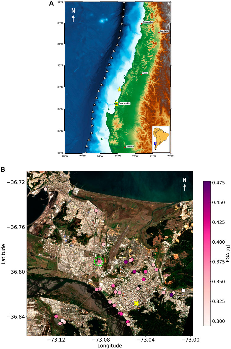
FIGURE 1. (A), upper panel: Shaded relief map of Central Chile. Red dots indicate major cities subjected to damages in the frame of the Maule 2010 Earthquake (epicenter depicted as a yellow star). The yellow rectangle represents Metropolitan Concepción, zoomed in the lower panel (B). Lower-right inset represents Central Chile (blue rectangle) within South America. (B) Satellite View of Metropolitan Concepción. Peak ground acceleration (PGA) color-coded circles show sites where surficial evidence of liquefaction was reported (Montalva et al., 2022). The PGAs were computed with Montalva et al. (2017) Ground Motion Prediction Equation. The dashed light-green circle encapsulates our study site, Los Presidentes. The yellow cross depicts the location of strong-motion station CCP, from which the earthquake ground motion was deconvolved to use as input for the site response analysis.

FIGURE 2

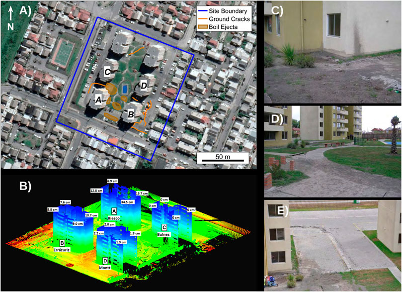
FIGURE 2. Summary of the damages at the Los Presidentes site. (A), upper left: Site boundary, damages in the form of ground cracks and boil ejecta. Only buildings A, B, C, and D are labeled because the northernmost ones were not built at the time of the earthquake. (B), lower left: A LiDAR image with the liquefaction-induced building settlements measured at the site (Robert Kayen, personal communication). The color palette indicates the distance between the laser sensor and the scanned surface. In this representation, red indicates larger distances, while blue corresponds to smaller distances. (C,D), top and middle right: Evidence of soil ejecta at the northeastern corner and inside the residential complex, respectively. (E), bottom right: Evidence of ground cracking between buildings A and C. Figure was extracted from Saldaña Sotelo (2023), and references therein.

2 Background and case study

The megathrust 2010 M_w 8.8 Maule Earthquake that struck South-Central Chile ruptured a mature seismic gap that was quiescent since the 1835 M_w 8.5 Concepción Earthquake (Campos et al., 2002; Ruegg et al., 2009; Moreno et al., 2010). The rupture propagated bilaterally north and south of the epicenter, covering an along-strike length of around 500 km. The reported damages spanned from the city of Valparaíso (33.0°S) to Temuco (38.7°S) (Bray et al., 2010; Assimaki et al., 2012). Figure 1A illustrates the main metropolitan areas affected by earthquake-induced damages. The city of Concepción (Figure 1B), located in South-Central Chile, experienced particularly strong ground motions. This behavior was attributed to site and basin effects that amplified the seismic load within the city (Assimaki et al., 2012; Montalva et al., 2016; Inzunza et al., 2019). Particularly, earthquake-induced liquefaction was reported throughout the city with varying levels of severity, including sediment ejecta, lateral spreading, flow failure, excessive settlements, surface cracks, and structural damage (Bray et al., 2010; Bray et al., 2012; Verdugo and González, 2015; Montalva et al., 2022).

Concepción is located on Pleistocene-Holocene sediments in a fluvial basin created by a horst-graben structure associated with NE-oriented normal faults that cut and displaced Upper Cretaceous to Pliocene sedimentary rocks on top of Upper Paleozoic granitic bodies (Galli, 1967; Vivallos et al., 2010). The basin infill is primarily made up of fluvial sand terraces that were formed due to the Bío-Bío River’s meandering after crossing the Coastal Cordillera toward its mouth at the Pacific Ocean. As a result of this process, metric banks of carefully selected sand grains were deposited, creating a relatively uniform unit (Montalva et al., 2016). Borehole, gravimetric, and tomographic studies have shown that the depth to bedrock is variable between outcropping rock up to 160 m, with an average basin thickness of 100 m (Poblete and Dobry, 1968; Inzunza et al., 2019). Geotechnically speaking (Montalva et al., 2016), the basin consists mostly of layers of poorly graded (SP) and silty sands (SM) that were uniformly deposited with non-plastic fines (approximately 22% fine content). This information was gathered from various boreholes conducted across the city. Additionally, layers of low-plasticity or no-plasticity silts (ML) ranging from 1 to 4 m thick can be found at different depths throughout the basin, indicating that they were deposited during a period of low velocity in the Bío-Bío River.

Figure 2A shows a satellite view of our case study area. At the time of the 2010 earthquake, there were four eight-story buildings on the site (towers A, B, C, and D); currently, there are six of them. Surficial evidence of liquefaction was reported on the site in the form of sediment ejecta (brown shapes in Figures 2A, C, D), ground cracking (orange lines in Figures 2A, E), and building settlements Bray et al., 2010, Bray et al., 2012). A Light Detection and Ranging (LiDAR) image (Figure 2B, Robert Kayen, Personal Communication, and in-situ reports (Bray et al., 2010; Bray et al., 2012) revealed that tower A experienced settlements ranging from 6.9 to 34.5 cm, while the ground surrounding the building settled roughly 22 cm. Tower B, on the other hand, experienced settlements ranging from 7.6 to 10.7 cm, while the surrounding ground settled about 18 cm. These large settlements caused extensive structural damage, leading to the demolition of both towers in 2013; they were subsequently reconstructed between 2016 and 2018. The other two towers, C and D, only experienced minimal settlements. Outside of the studied area, no evidence of liquefaction was reported. In this study, we have focused our region of interest to the area between buildings A and B (Figure 3A). Six geotechnical tests were conducted in this region - three SPT, and three CPT boreholes (cyan stars in Figure 3A). A comprehensive geotechnical characterization of the site, derived from the data obtained through the boreholes, is described in Saldaña Sotelo (2023); Saldaña et al. (2023).

FIGURE 3

FIGURE 3. (A), left: Schematic view of the study site. Magenta triangles depict the positions of seismic sensors, black lines connecting them show the station pairs from which dispersion curves shown in (B) were retrieved. The dashed red line represents the T-T′ cross-section employed in the numerical model. (B), right: Distribution of all Rayleigh Wave dispersion curves across the study site. Cyan stars illustrate the location of the geotechnical borehole tests.

3 Theory

3.1 Retrieving dispersion curves from ambient noise data

In the subsequent section, we introduce the seismic interferometry technique in a broad way. First, we explain how through cross-correlations in the time-domain, a representation of the Green Function can be obtained. Following this, we explain the SPAC technique and the assumptions for which it is valid. Finally, we establish a connection between the time-domain cross-correlation method and the frequency-domain SPAC method.

The noise wavefield refers to the combination of seismic waves caused by ambient vibrations of both natural and anthropogenic origin, such as tides, oceanic waves, meteorological phenomena, heavy machinery, and vehicles (Asten and Henstridge, 1984; Bonnefoy-Claudet et al., 2006). This wavefield is primarily composed of surface waves (Chávez-García and Luzón, 2005; Bonnefoy-Claudet et al., 2006). The dispersive nature of the surface waves allows us to illuminate the Earth’s internal structure through the seismic interferometry technique (Curtis et al., 2006). Under the assumption that the noise wavefield is diffuse (i.e., waves with uncorrelated random amplitudes and phases propagate in all directions, Weaver, 1982; Lobkis and Weaver, 2001), the Green’s Function and the group or phase velocity dispersion curve between two receivers can be calculated by averaging the correlograms over time (Shapiro and Campillo, 2004; Wapenaar et al., 2010). In spite of the strong assumptions made about the wavefield, the widespread success of ambient seismic noise methodologies in recent years has demonstrated their effectiveness in a variety of applications, ranging from soil structure characterization to lower crust/upper mantle tomographic models (e.g., Shapiro et al., 2005; Ritzwoller et al., 2011; Ward et al., 2013; Ma and Clayton, 2014; Inzunza et al., 2019). The bandwidth of the retrieved dispersion curves is primarily constrained by instrumental characteristics, the interstation distance between the receivers, and the deployment time of the seismic array. The number of stacked correlograms, whose duration is frequency-dependent, increases the signal-to-noise ratio (Bensen et al., 2007). In fact, for shallow imaging (i.e., $<100$ meters), recording for a few hours should suffice (e.g., Picozzi et al., 2009; Pilz et al., 2012). On the other hand, researchers have stacked years of data to obtain dispersion curves for deeper explorations (e.g., Ward et al., 2013; Ma and Clayton, 2014).

The aforementioned approach is based on time-domain cross-correlation. However, a similar method, called SPatial AutoCorrelation (SPAC, Aki (1957), states that if the noise wavefield is stochastic and stationary in space and time, the azimuthal average of the cross-correlation in the frequency domain (i.e., the cross-coherence CC) for a fixed distance r at frequency ω is related to the Rayleigh wave phase velocity c(ω) by

$\bar{\rho }\left(r,\omega \right)=A{J}_0\left(\frac{\omega r}{c\left(\omega \right)}\right),(2)$

where J₀ represents the zero-th Bessel function of the first kind, and A is an amplitude factor that considers attenuation and normalization errors in the CC (e.g., Menke and Jin, 2015). It is noteworthy that the azimuthal average can be replaced by the time average if we consider that the noise wavefield is diffuse (Aki, 1957; Chávez-García et al., 2005). This implies that the cross-correlation and SPAC methods are equivalent (Chávez-García and Luzón, 2005; Tsai and Moschetti, 2010). With that in mind, the time-averaged CC is defined as (Ohori et al., 2002; Wapenaar et al., 2010; Xu et al., 2021)

${\rho }_{ij}\left(\omega \right)=⟨\frac{\mathfrak{R}\left(S_{ij}\left(\omega \right)\right)}{\sqrt{S_{ii}\left(\omega \right)S_{jj}\left(\omega \right)}}⟩,(3)$

where $\mathfrak{R}\left(S_{ij}\right)$ is the real part of the cross power spectral density (PSD) between station pair i and j, S_ii and S_jj are the individual PSDs, and the ⟨⋅⟩ operator denotes averaging over time segments. For each pair of simultaneous recordings, the CC is calculated with Equation 3, and substituted into Equation 2. It is clear from these equations that the relationship between the data and the phase velocity is nonlinear. Still, the dispersion curve c(ω) can be retrieved through the zero-crossings (Ekström et al., 2009; Ekström, 2014) or by fitting a Bessel function to the CC waveform (e.g., Menke and Jin, 2015; Pilz et al., 2017; Olivar-Castaño et al., 2020).

3.2 Retrieving ground profiles from dispersion curves

The relationship between the dispersion curve and a one-dimensional ground profile is also nonlinear. Furthermore, the dispersion curve includes contributions from both fundamental and higher modes, which cannot be trivially separated. The curve that is composed of this superposition of modes is known as the apparent dispersion curve. This curve is related to each mode through their respective medium response functions (Harkrider, 1964; Tokimatsu et al., 1992; Ohori et al., 2002). Therefore, the nonlinear inverse problem relating the apparent dispersion curve and the ground profile can be solved using adequate methods, such as the simplex downhill method (Nelder and Mead, 1965) or a genetic algorithm (Yamanaka and Ishida, 1996; Parolai et al., 2005).

The genetic algorithm employed in this research is a nonlinear, partially probabilistic approach that aims to explore the entire parameter space in order to find the optimal solution (i.e., the space within the predefined lower and upper bounds for density and P-S wave velocity). Since each inversion is defined by a random seed, all resulting solutions are unique, even if they start with the same parameterization. Consequently, there are two significant issues regarding the inverse problem solution and parameterization: the non-uniqueness of the solution and how well it is constrained by the available data. The first issue implies that many different ground profiles may fit the data reasonably well, making it difficult to determine a single ‘true’ solution. The second issue highlights the limitations of dispersion curve data and how this data constrains each layer’s thickness and the maximum depth exploration. A layering-by-ratio scheme was designed to address these issues Cox and Teague (2016); Vantassel and Cox (2021). This approach allows for the exploration of various parameterizations, with different numbers of layers, in order to determine the optimal number of layers that suitably fit the data, preventing over or under-parameterization. Moreover, it ensures that no layers begin below the wavelength-defined spatial resolution. The best-constrained solution can be selected by minimizing the misfit between the data and the prediction, and a measurement of the inter-parameterization uncertainty can be obtained from the N-lowest misfit solutions (e.g., N = 10, 100).

4 Characterization of the site velocity structure

4.1 Data and methods

In the frame of this study, we conducted five geophysical surveys from November 2021 to December 2022. Three-component high-frequency seismic Tromino^® instruments, with a sampling rate of 512 Hz, were deployed at the study site to record the ambient seismic wavefield at a total of 50 station positions (magenta triangles in Figure 3A). The instruments were configured to record synchronously for a duration of approximately 40 min at each position. For each pair of simultaneous recordings (black lines in Figure 3A), the CC was calculated with Equation 3 using the Welch Method (Welch, 1967). This method involves computing periodograms from detrended segments of 60 s in length, with a 50% overlap between segments. Additionally, a 5% cosine taper was applied to both ends of each segment, followed by a one-bit normalization filter. This procedure reduces spectral leakage and increases the signal-to-noise ratio (Bensen et al., 2007). Finally, the CC was smoothed using a moving-average filter and substituted into Equation 2. The lower and upper phase velocity limits for the solution were set to 100 [m/s] and 400 [m/s], respectively, based on results from previous surveys (Montalva et al., 2022; Saldaña et al., 2023; Saldaña Sotelo, 2023). We defined the minimum resolvable wavelength, λ_min, as half the interstation distance (r/2). Due to the different interstation distances, we manually defined the frequency band for the 198 CC waveforms produced. Furthermore, we conducted a visual inspection of the resulting dispersion curves, obtained using the methodology of Menke and Jin (2015), discarding any curves that fit the CC waveforms poorly and outliers corresponding to geologically-implausible interpretations (i.e., they do not align with the fluvial sand-filled Concepcion basin). A subset of 123 curves, presented in Figure 3B, aligned with the aforementioned criteria. The minimum and maximum velocities are 116 and 320 [m/s], respectively, while the frequency range spans from 2.85 to 25 Hz. The majority of dispersion curves fall within the 6–16 Hz frequency band, and are representative of very soft, shallow conditions. Subsequently, each dispersion curve is transformed from linear-frequency to the log-wavelength domain. Given that the variation of phase velocity as a function of wavelength is less than as a function of frequency, this transformation reduces the gap between points in the dispersion data without needlessly increasing the number of samples (Vantassel and Cox, 2021).

We inverted ground profiles for each dispersion curve using a generic algorithm (Yamanaka and Ishida, 1996; Parolai et al., 2005) with parameterizations consisting of 3, 4, and 5 layers for each curve, with the deepest layer representing the half-space base. The V_s lower and upper bounds of each layer (regardless of their depth) were set to depend on the lower and upper values of the dispersion curve, ranging from approximately 100 to 350 m/s for the upper sedimentary layers and up to 450 m/s for the half-space layer. As the generic algorithm is part-probabilistic, each dispersion curve was inverted using 12 seeds, resulting in a total of 36 inversions for each curve considering the different numbers of layers used. Then, through visual inspection of the ground profiles and their goodness-of-fit to the data, we determined the number of layers most adequate for each curve and identified the representative ground profile as the one exhibiting the lowest misfit with respect to the dispersion curve. Furthermore, from the 12 solutions, we estimated the inter-model uncertainty by calculating ${\sigma }_{ln,v_s}$, representing the logarithm of the standard deviation of the velocity.

4.2 Inverted ground profiles

Figure 4 displays three representative ground profile solutions, their uncertainties, and the dispersion curve fit obtained through the aforementioned procedure. Subsequently, we narrow our focus on the first 30 m of the V_s profiles, as the deeper structure is poorly resolved by the frequency range of our phase velocity data. It can be seen that the thickness of the upper layers decreases as the interstation distance decreases because the wavelengths constrained by the dispersion curves become shorter. Additionally, the uncertainties (blue dashed lines in Figure 4A) tend to increase near the depths corresponding to layer interfaces. This happens because the trade-off between layer thickness and V_s cannot be resolved using only dispersion data. Nevertheless, the ground profile uncertainties are within the expected range for surface wave surveys (Vantassel and Cox (2021) and references therein).

FIGURE 4

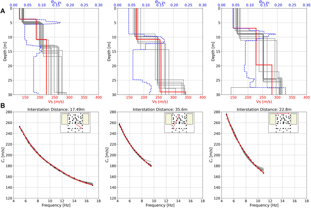
FIGURE 4. (A) Top panels: The ground profiles inverted from the dispersion curves displayed in the lower panels. Grey profiles show the lowest misfit solution for each seed. The red profile is the lowest-misfit solution for all seeds. The dashed blue line represents the logarithm of the standard deviation of V_s. (B) Lower panels: Dispersion curve fit (dotted black line) by each ground profile. Colors represent the same as at the top panels.

4.3 Merging scheme

We used a simple merging scheme to quantify the spatial variability of V_s from the ground profiles, reminiscent of the approximative tomographic inversion proposed in Kissling (1988). First, we divided the site into a rectangular grid of 35 m in the x direction and 42 m in the y direction (Figure 5). Assuming that the surface waves travel along straight lines linking each pair of receivers, the velocity profile corresponding to each grid cell is obtained by weighting all the ground profiles corresponding to pairs of stations whose interstation path passes through it. The weighting scheme takes into account the length of each ray within the grid cell and the ${\sigma }_{ln,v_s}$ of each profile. In other words, the ground profile associated with the ray with the longest length within a specific grid cell carries greater weight than rays crossing shorter distances in the same grid cell. Additionally, ground profiles with lower values of ${\sigma }_{ln,v_s}$ for a given depth also have greater weight. Then, for a given cell that is crossed by n rays of cell length l and logarithmic standard deviation σ^z at a given depth, the shear-wave velocity at depth z, V^z, is given by

$V^z={\displaystyle \sum _{j=1}^n}\frac{l_j{V}_j^z{\left({\sigma }_j^z\right)}^{-1}}{{\sum }_{k=1}^n{l}_k{\sum }_{k=1}^n{\left({\sigma }_k^z\right)}^{-1}},(4)$

where the subindex s of the shear-wave velocity term V_s is omitted here for clarity. Equation 4 ensures that rays covering more distance within a cell carry more weight, that short interstation distance models have more weight at shallow depths, and that large interstation distance models have more weight at greater depths.

FIGURE 5

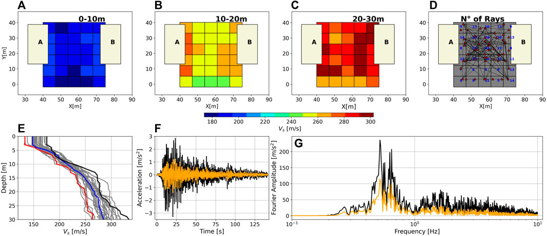
FIGURE 5. The velocity structure of the site calculated by the weighting scheme. (A–C), leftmost top panels: Average V_s structure at depths of (0–10 [m]), (10–20 [m]) and (20–30 [m]), respectively. In (A–C), the X and Y coordinates are within the coordinate system of Figure 3A. (D), top right: Distribution of ground profiles averaged on each grid to obtain the weighted ground profile. (E), lower left: The weighted ground profiles of all grids. Three representative profiles of different ground conditions are depicted with red, blue, and black lines. The red velocity profile, which represents free-field conditions, is used for the ESSRAs. (F, G), rightmost lower panels: Black and orange ground motion and their Fourier spectrums depict the CCP EW station recording and its deconvolution to 50 m depth, respectively.

4.4 Resulting velocity structure and representative profiles

Figures 5A–C display the average velocity structure of the site at depths of 0–10 [m], 10–20 [m], and 20–30 [m]. Generally, lower velocities are observed in the shallow structure (Figure 5A), with increasing velocities at greater depths (Figures 5B, C). Notably, the grid cells near the towers show relatively high velocities at all depths with respect to the middle and southernmost cells. This can be attributed to the fact that the southernmost part of the study area is located near public streets, which were likely not consolidated by heavy machinery before the building reconstruction. On the other hand, the cells in the middle are in an area that was likely consolidated and refilled before the reconstruction of the towers, but to a lesser extent than the cells adjacent to the structures. Moreover, the weight of the buildings themselves may also affect the velocity structure of the adjacent cells. Figure 5E shows the weighted ground profiles for all the grids (grey profiles). The black profile represents cells directly adjacent to the buildings. The blue profile represents cells in the ground area between the buildings. The red profile represents cells south of the buildings. As severe liquefaction was observed near buildings A and B in 2010, the red profile (soils not consolidated by heavy machinery prior to reconstruction) is considered the most representative of the free-field natural conditions that existed for our simulations.

5 Numerical model setup

We perform ESSRA using the Open System for Earthquake Engineering Simulation (OpenSEES) finite-element framework (McKenna, 2011) and the Scientific Toolbox for OpenSEES (Petracca et al., 2017). The wave propagation over fluid-saturated porous media is solved in a 2D domain under plane-strain conditions. We consider the cross-section T-T′ depicted in Figure 3A, a domain of 140 m in length in the x-direction and 50 m in depth in the z-direction, as shown in Figure 6A. In our modeling, we did not account for the influence of building’s load. To enforce free-field conditions at the lateral boundaries of the model, we model free-field columns of 10 m length in the x-direction and 10,000 m size in the out-of-plane-direction, and tie the displacement degree-of-freedom to enforce periodic boundary conditions, in a very similar manner to what is performed. The nodes at the base of the model were fixed in the z-direction, under the assumption that the domain is underlain by an elastic homogeneous half-space, and they were forced to move horizontally in the same direction by tying them to the lower-left node. The ground motion was input at this lower-left node as a force time history with a Lysmer-Kuhlemeyer dashpot (Lysmer and Kuhlemeyer, 1969; Joyner and Chen, 1975), and propagated to the constrained base nodes and across the domain. The LK dashpot method requires to input a coefficient $c={\rho }_b{V}_{s_b}{A}_{\mathit{elem}}$, with ρ_b = 2.0[g/cm³] and $V_{s_b}=339[m/s]$ being the density and shear-wave velocity of the underlying medium (i.e., the elastic homogeneous half-space) and A_elem = 10*10000 m². As neither borehole nor outcrop bedrock seismic recordings were available near our study site, the ground motion at the base was estimated by applying simple linear deamplification, to a depth of 50 m, of the ground motion recorded at station CCP (see Figure 1 for station location; Figures 5F, G for the station ground motion). As mentioned earlier, our profiles are well-constrained only until a depth of 30 m. To address this issue, we created a joint profile by taking the median of all of our non-weighted ground profiles until 30 m, and using the profile derived for the Concepción basin from Inzunza et al. (2019) below this depth. The merged profile is shown in Table 1.

FIGURE 6

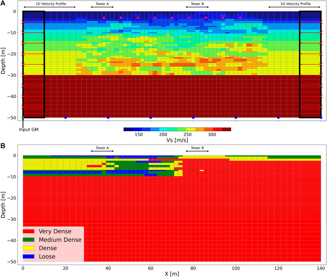
FIGURE 6. Benchmark finite element model realization of the T-T′ cross-section defined in Figure 3. (A), top panel: V_s random field obtained using ${\sigma }_{ln,v_s}=0.075$. Free-field columns at the lateral boundaries are depicted in thick black rectangles. The red arrows start and end at the main and constraint nodes, respectively. Input ground motion is applied at the green node in the lower-left corner. Base nodes (blue) are constrained to the green node. The recorder nodes at a depth of 3 m are depicted as magenta triangles and are further analyzed in Figure 9. (B), lower panel: D_r structure of the cross-section (Saldaña et al., 2023; Saldaña Sotelo, 2023).

TABLE 1

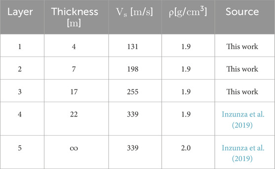
TABLE 1. Joint ground profile obtained by merging the median profile from this work and the uppermost two layers of the profile derived in Inzunza et al. (2019).

Effective stress conditions are enforced using stabilized-single-point quadrilateral u − p elements (SSPQUADUP, McGann et al., 2012), which are based on the u − p formulation. This formulation assumes that saturated soils are a continuum composed of a solid and a fluid phase, with the displacement of the solid phase u and the pore-fluid pressure p of the fluid phase being the main variables. These underlying assumptions are valid for most earthquake and soil dynamics problems (Biot, 1956; Zienkiewicz and Shiomi, 1984). SSPQUADUP elements include an additional pressure degree of freedom. As the groundwater table at the site varies from roughly 0.5–1.5 m (Saldaña et al., 2023; Saldaña Sotelo, 2023), we fixed the pore-water pressure degree-of-freedom at the surface level.

To model the elastoplastic behavior of the sands in the shallower 30 m, we used the PressureDependentMultiYield03 model (Khosravifar et al., 2018). This multi-yield surface model was originally designed to capture the cyclic mobility and post-liquefaction accumulation of shear strain on sands and has been updated to account for the influence of the number of loading cycles on liquefaction triggering. A thorough description of the model formulation can be found in Parra-Colmenares (1996); Yang et al. (2003); Khosravifar et al. (2018). We highlight from the abovementioned literature that (1) the model assumes that elastic and plastic deformations occur simultaneously in the soil, and the elastic behavior is linear and isotropic, while the plastic behavior is nonlinear and anisotropic, and (2) the soil nonlinear shear stress-strain response is defined in the octahedral space in the following manner: the pressure-dependent small-strain shear modulus $G_{\mathit{max}}^p$ is defined by

$G_{\mathit{max}}^p=G_{\mathit{max}}{\left(\frac{p^{\prime }}{p_r^{\prime }}\right)}^d,(5)$

where G_max is the input shear modulus computed with Equation 1 at a reference effective confining stress $p_r^{\prime }$, d is the pressure-dependent coefficient set to 0.5, and p′ is the effective confining stress that varies during the earthquake loading. Thus, shear modulus reduction curves are computed using a hyperbolic relationship given by

${\tau }_{\mathit{oct}}=\frac{G_{\mathit{max}}^p}{1+\frac{{\gamma }_{\mathit{oct}}}{{\gamma }_r}{\left(\frac{p_r^{\prime }}{p^{\prime }}\right)}^d}\left({\gamma }_{\mathit{oct}}\right),(6)$

Where τ_oct is the octahedral shear stress, γ_oct is the deviatoric strain in the octahedral space, and γ_r is a parameter that constrains the shape of the backbone curve. Equation 6 describes the shape of the hysteretic loops for a given effective stress, small-strain shear modulus at a given pressure (given by Equation. 5), and seismic excitation. Most of the model input parameters apart from G_max and the Bulk Modulus at a reference pressure B_r, which can be computed from G_max, have already been calibrated by the developers for different relative densities. Therefore, we mapped the D_r values from the geostatistical model described in Saldaña Sotelo (2023); Saldaña et al., 2023 into our domain (Figure 6B). Table 2 summarizes the model parameters used for our analyses.

TABLE 2

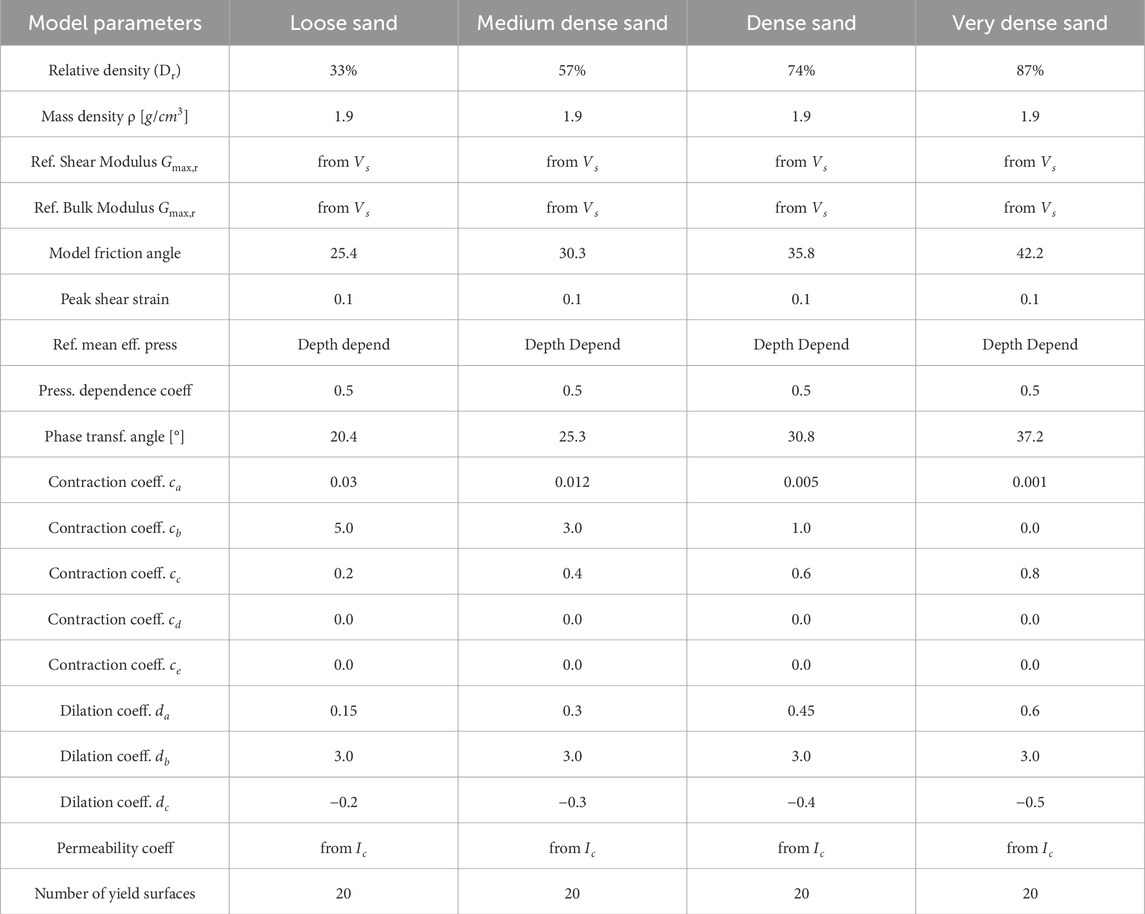
TABLE 2. Pressure Dependent Multi Yield 03 model parameters employed in this research.

To simulate V_s heterogeneity and wave attenuation, we followed the method of de la Torre et al. (2022a); de la Torre et al. (2022b). We generated perturbations of the 1D V_s profile shown in Figure 5E, using spatially anisotropic correlated Gaussian random fields with varying ${\sigma }_{ln,v_s}$ values, to simulate different levels of heterogeneity. The parameters that we need to define to achieve this are the following:

• The logarithm of the standard deviation of the velocity ${\sigma }_{ln,v_s}$: Here we set five different values: 0.075, 0.125, 0.175, 0.225, and 0.275, to simulate conditions with very low to high variance. Values mentioned in de la Torre et al. (2022a), and references therein range from 0.1 to 0.37. The ${\sigma }_{ln,v_s}$ values obtained for our profiles in Figure 4 vary roughly from 0.04 to 0.23, consistent with the aforementioned literature and the values chosen. We run 20 simulations per level of variance, resulting in a total of 100 simulations.

• The horizontal r_H and vertical r_V correlation lengths were set to 15 and 2 m. This is within the bounds of values previously used for generating heterogeneous V_s random fields. (Popescu, 1995; Assimaki et al., 2003; de la Torre et al., 2022a). An exponential function was used to simulate the spatial correlation.

Additionally, a zero-variance zone of 25 m length was established at the lateral boundaries, where the 1D deterministic soil profile is valid. Figure 6 shows the benchmark V_s realization for ${\sigma }_{ln,v_s}=0.075$. Lastly, a single homogeneous elastic layer of V_s = 339 m/s was used for the subdomain within 30 and 50 m depth. We implemented the procedure of Ramirez et al. (2018); Tiznado et al. (2021) to determine the vertical size of the elements efficiently. For small-strain problems, the maximum vertical element size, h_max, depends on the V_s value of the element and the maximum frequency of the input motion: $h_{\mathit{max}}=\frac{V_s}{4f_{\mathit{max}}}$. As the shear modulus degrades in nonlinear problems, this implies that V_s will decrease as the simulations progress. Therefore, to ensure that our elements do not exceed their theoretical maximum size, we further divided h_max by a factor of 4 to account for this phenomenon and guarantee that a sufficient number of elements cover one wavelength at all times.

6 Simulation results

We now describe and analyze the simulation results from five simulation outputs:

• The shear strain γ.

• The volumetric strain ϵ_v, defined as the mean of the vertical and horizontal strains.

• The excess pore-water pressure ratio r_u, defined as the difference between the current and initial pore-water pressure divided by the overburden effective stress.

• The vertical settlements u_z.

• The horizontal acceleration a_x

Threshold values previously defined in the literature for liquefaction triggering are between 80% and 100% for r_u, and between 3% and 5% for the shear strains (Ishihara, 1993; Boulanger et al., 1998; Bray and Sancio, 2006).

6.1 Benchmark simulation

Figure 7 shows the maximum shear strain γ, maximum volumetric strain ϵ_v, excess pore water pressure ratio r_u, maximum horizontal acceleration a_x, and vertical settlement u_z for the benchmark model realization shown in Figure 6. We focus on three representative nodes, which are depicted as white circles 1, 2, and 3 in Figure 7. For the zone surrounding representative node 1, liquefaction of a loose sand layer (see Figure 6B) occurs at depths between 7 and 8 m due to the accumulation of large strains (Figures 7A, B) and r_u values exceeding 100% being located in this part (Figure 7C). The highly nonlinear hysteretic loops of the stress-strain curve and the r_u time series are also consistent with liquefaction phenomena (Figure 8A). Moreover, a steep gradient of horizontal accelerations is observed below the node (Figure 7D).

FIGURE 7

FIGURE 7. Maximum shear strain (A), volumetric strain (B), excess pore-water pressure ratio (C), horizontal acceleration (D), and settlements (E) for the benchmark model realization shown in Figure 6. The magenta numbered circles represent the locations of the three nodes depicted in Figure 8.

FIGURE 8

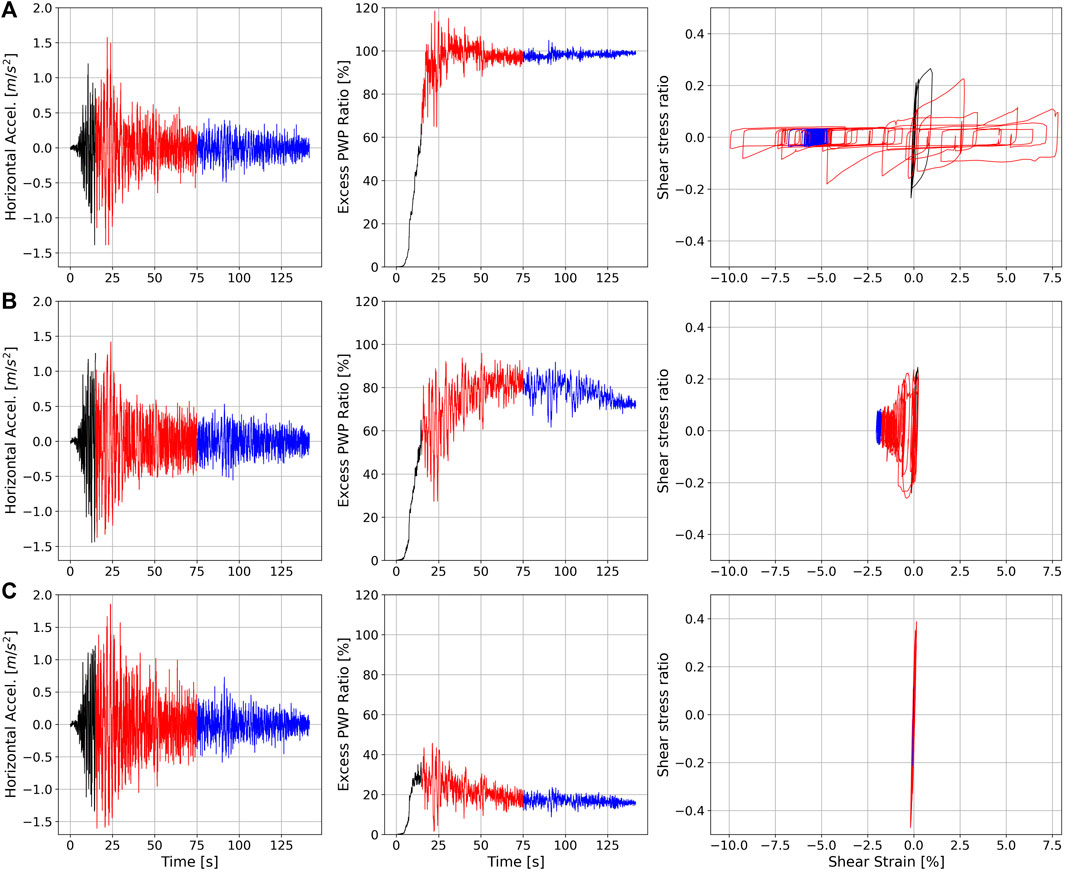
FIGURE 8. Recorder acceleration, excess pore-water pressure, and stress-strain time series of the numbered nodes of Figure 7. (A), top: Node 1. (B), middle: Node 2. (C), bottom: Node 3. The time series’ black, red, and blue color codes represent the first 15 s of motion, from 15 to 75 s, and from 75 to the end of motion.

For the zone surrounding representative node 2, we observe slightly smaller maximum r_u values ($\sim 90-100\%$, Figure 7C) and maximum shear strains in the range of 2–4% (Figure 7A). These r_u and shear strain values are close to the previously stated threshold values (Ishihara, 1993; Boulanger et al., 1998; Bray and Sancio, 2006). The stress-strain response recorded is nonlinear (Figure 8B), but to a considerably lesser extent than node 1. Furthermore, the maximum volumetric strains are negative (indicating contraction) near node 2, but the surface values are positive (indicating dilation) (Figure 7A). The area around node 2 is the one that exhibits the largest vertical settlements, reaching roughly 50 mm (Figure 7E).

As for the zone surrounding representative node 3, no liquefaction occurs. Indeed, r_u values do not exceed 50% (Figure 7C), the stress-strain behavior is close to linear (Figure 8C), no significant settlements are observed (Figure 7E), and the maximum accelerations are significantly higher than in the zone around node 2 (Figure 7D), implying that this zone did not experience significant soil softening. As shown in Figure 6B, node 3 is embedded in a zone of dense sands, which are less susceptible to liquefaction compared to the layers in which nodes 1 and 2 are situated.

6.2 Assessing the effect of V_s variability on key dynamic properties

In Figure 9, we plot, for different levels of ${\sigma }_{ln,v_s}$, the median maximum γ, ϵ_v, r_u, and u_z of all simulations as a function of the distance along the cross-section at a depth of 2 m. The cross-section’s nine nodes—five positioned to the west and four to the east—display distinct behaviors. Consequently, we conduct separate analyses for the two cases. For the western nodes, the high r_u (80–100%) values for all ${\sigma }_{ln,v_s}$ levels are indicative of liquefaction behavior. Particularly, we can see that an increase in ${\sigma }_{ln,v_s}$ leads to a decrease in the median maximum γ and ϵ_v. In a similar manner, a slight reduction in the median maximum u_z is observed at the nodes x = 46 [m] and x = 54 [m] as ${\sigma }_{ln,v_s}$ drops. This tendency is not observed for the rest of the western nodes, and the median maximum u_z values are very similar. Additionally, no significant changes in the median maximum r_u values are observed.

FIGURE 9

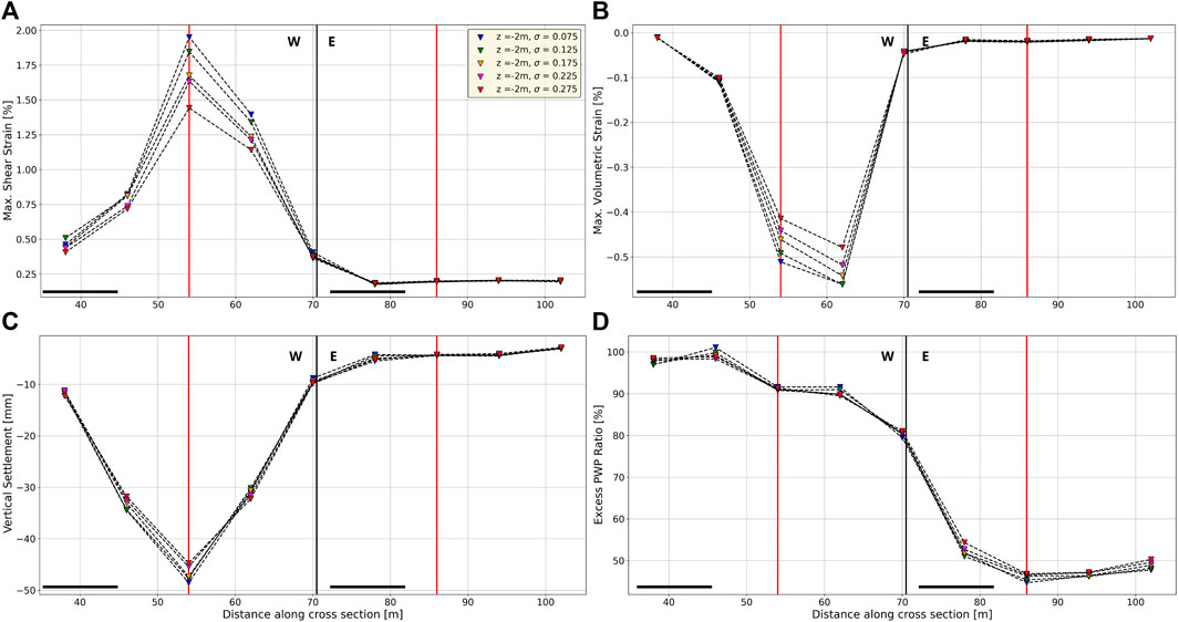
FIGURE 9. Median of the Max. Shear strain (A), top left; max. Volumetric strain (B), top right; max. PWP ratio (C), bottom left; and vertical settlements (D), bottom right, at different levels of ${\sigma }_{ln,v_s}$ across the T-T′ cross-section. Nodes are located at a depth of 2 m. Thick black vertical line divides the western from eastern nodes. Thick red vertical lines depict the location of the western and eastern nodes analyzed in Figure 10 and Supplementary Figure S5. Horizontal black lines near the x-axis represent the locations of towers A and B relative to the cross-section.

For the eastern nodes, the low r_u (45–50%) values and the developed small strains and settlements indicate that no liquefaction occurred. Furthermore, we appreciate very slight variabilities in the soil response for different levels of ${\sigma }_{ln,v_s}$. Only a slight increase in the median maximum r_u values with increasing ${\sigma }_{ln,v_s}$ is observed, which is a contrary behavior to what is seen in western nodes. Anyhow, variations on ${\sigma }_{ln,v_s}$ did not signify a change in the eastern nodes from non-liquefaction to liquefaction behavior. Although the values are slightly different, a very similar behavior for the western and eastern nodes is observed at depths of 4 and 5 m (Supplementary Figures S1, S2).

Figure 10 shows the time series of the aforementioned variables for all the simulations (grey lines) and the median time series at different levels of ${\sigma }_{ln,v_s}$ for the western node x = 54 [m] (see Figure 9 for node location). This is the node that exhibited the largest median maximum shear strain and settlements. Overall, we see that all the median time series closely follow each other in the first 20 s, when r_u values are not large. After the 20 s, and even more markedly at around 45 s (i.e., when r_u stabilizes and stops increasing), differences between the ${\sigma }_{ln,v_s}$ levels become apparent. In the same line, we see that all simulations (regardless of ${\sigma }_{ln,v_s}$) follow the pattern of permanent strain accumulation when high pore-water pressures are developing. This implies that liquefaction behavior occurs regardless of the simulation ${\sigma }_{ln,v_s}$ level. Additionally, the same tendency of greater ${\sigma }_{ln,v_s}$ leading to smaller strains and settlements observed in Figure 9 is noted for the median time series. It can be appreciated as well that starting from t > 40s, the higher median r_u values happen for ${\sigma }_{ln,v_s}=0.075$, but the increase is slight.

FIGURE 10

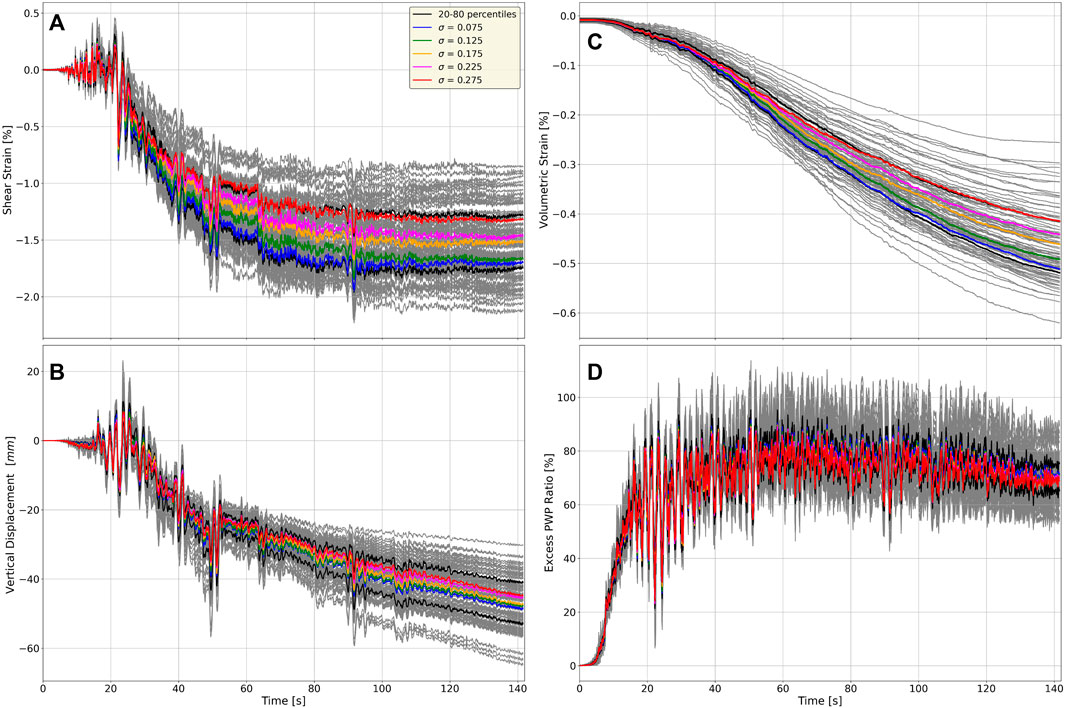
FIGURE 10. All simulations of shear strain (A), volumetric strain (B), vertical displacement (C), and excess pore-water pressure ratio (D) time series computed for the node at the western node at position x = 54 and depth of 2 m, depicted in Figure 9. Color-coded time series represent the median time series at different levels of ${\sigma }_{ln,v_s}$. Black curves represent all simulations’ 20-th and 80-th percentile time series.

Black curves in Figure 10 show all model simulations’ 20-th and 80-th percentiles. For the strains and r_u time series, ${\sigma }_{ln,v_s}=0.075$ and ${\sigma }_{ln,v_s}=0.275$ curves follow closely the 80-th and 20-th percentile curves, respectively. On the other hand, we see from the vertical displacement time series that the percentile curves are farther off from the median curves than for the strain and r_u time series. Actually, the settlement u_z (i.e., the last value of the time series) for the 20-th and 80-th percentiles considerably varies from 41 to 53 mm. We can also see that the volumetric and vertical displacements are still increasing at the last time step. This could indicate that flow is still occurring after the strong motion has ended, and hence larger settlements could be obtained by increasing the simulation time. A similar pattern is observed for the time series at depths of 4 and 5 m (Supplementary Figures S3, S4).

For comparison, we also show the time series for the eastern node x = 86 [m] (Supplementary Figure S5). From here, we mention two noteworthy points: The first is that shear strain, pore-water pressure ratio, and vertical displacement median time series for each ${\sigma }_{ln,v_s}$ are much more stacked together than in the previous case. Additionally, we appreciate more variability in the volumetric strains, although the maximum magnitude of the strains accumulated is smaller than 0.05. With that in mind, even though the 20-th and 80-th of volumetric strains and vertical displacements are farther off from the median curves, their values are very small. The second is that no liquefaction behavior is observed even for the most extreme outliers simulations (i.e., the ones that exhibit the largest r_u). This is in agreement with what we had shown for the eastern nodes in Figure 9.

7 Discussion

Our findings indicate distinct responses between western and eastern nodes due to the varying levels of V_s spatial variability. While strains and settlements tend to decrease as variability increases for the western nodes, the response of the eastern nodes remains relatively unchanged. In Figure 10, we see that the western node was subjected to large plastic deformations across all ${\sigma }_{ln,v_s}$ levels, while Supplementary Figure S5 demonstrates minimal deformations for all simulations at the eastern node. From this, and recalling from Figure 6 that the shallow western part of the domain corresponds to soil units with low relative density, and the shallow eastern part of the domain corresponds to units with high relative density, it can be inferred that V_s spatial variability may not alter the soil’s intrinsic response to liquefaction. This response is likely primarily controlled by the soil’s mechanical properties and the earthquake loading. In other words, our results support the notion that V_s spatial variability does not play a primary role in liquefaction triggering, but rather influences the liquefaction response when liquefaction is already ongoing.

We propose a physical explanation for the decrease in liquefaction-induced settlements and strains as ${\sigma }_{ln,v_s}$ increases. As seen in Figure 10A, the median curves diverge as nonlinear behavior increases (i.e., plastic deformation develops during the simulation). We can infer that the more nonlinear the behavior of the soil is, the increased importance of ${\sigma }_{ln,v_s}$ becomes apparent. Certainly, it is known that for a given shear-wave velocity value, the soil damping increases with larger shear strains (Hashash and Park, 2001; 2002). Therefore, if variability increases, the overall soil stiffness decreases, intensifying the damping and reproducing the observed deformation patterns. It should be noted that this pattern depends on the median V_s values and the confining pressure of the soil units. If V_s is high and the soil unit is deep, the damping will be lower due to the increased shear strength of the soil, reducing the importance of ${\sigma }_{ln,v_s}$. See, for instance, Supplementary Figure S6, which displays the shear-strain time series of node number 1 from Figure 7, where significant liquefaction was observed between 7 and 8 m depth. Even though larger shear strains close to 10% are appreciated, the median time series do not exhibit a clear relationship between ${\sigma }_{ln,v_s}$ and the developed shear strains. In summary, we propose that the influence of ${\sigma }_{ln,v_s}$ on the liquefaction response becomes relevant in the following circumstances:

1. The ground motion intensity is strong enough to trigger nonlinear behavior and significant r_u values.

2. The mechanical properties of the soil allow liquefaction to occur.

3. The median V_s of the soil at a given depth is sufficient to allow significant damping when subjected to large (e.g., $>1$) shear strains for a given ground motion intensity.

In terms of liquefaction-induced settlements, one of the most detrimental liquefaction hazards, our results show that the effect of V_s spatial variability on the median computed settlements was consistent but slight. However, the settlements’ 20-th and 80-th percentiles are 41 and 53 mm, respectively. This implies that V_s variability may significantly influence the computed settlements. Therefore, it is crucial to constrain the velocity structure of a site accurately in order to gain a better insight into the liquefaction response of a case study. With this in mind, we identified three distinct V_s profiles consistent with the site’s geophysical and geotechnical characteristics within our small study site. For bigger soil domains (e.g., Pretell et al., 2021; Qiu et al., 2023, we can expect to see even more diversity on V_s signatures.

We note that the calculated maximum shear strains near the surface are not larger than 3%, which is not considered to be exceedingly large. Saldaña Sotelo (2023); Saldaña et al. (2023) conducted ESSRAs at the same study site and obtained maximum surface shear strains near the surface up to 10%. Additionally, simulations of Luque and Bray (2017) on two buildings - that exhibited liquefaction-induced settlements during the Canterbury Earthquake Sequence of 2010–2011 - reached maximum shear strains beneath the buildings of around 8%. We suggest that the effect of V_s heterogeneities on near-surface deformations may be more significant in these cases compared to our study.

Even though it was not our primary research goal, we compared the computed settlements at the representative western and eastern nodes with the ground settlements reported in Bray et al. (2010, 2012) (Table 3). Our average settlements for both nodes are significantly lower than the reported values, especially for the eastern node, where no liquefaction behavior was captured in our simulations. We suggest motives for that discrepancy. Recent studies have shown that including structures in the simulations may greatly increase the vertical settlements in the proximity (Bray and Luque, 2017; Saldaña et al., 2023; Saldaña Sotelo, 2023). At our study site, Saldaña Sotelo (2023); Saldaña et al. (2023) calculated the liquefaction-induced ground settlements from the available CPT data using Zhang et al. (2002) simplified methodology, obtaining values from 10 to 37 mm. These values also do not match the observations, but are more in alignment with what we obtained. Vertical settlements computed with empirical relationships exhibit mismatches with observations because they (1) assume free-field conditions, (2) only consider volumetric-induced settlements, and (3) cannot reproduce the complex system response as numerical modeling does. While our modeling considers volumetric and shear-induced settlements and reproduces the system response, it was conceived under a free-field assumption. We therefore suggest that not accounting for the buildings’ load is the principal reason our simulations underestimate the settlements. Other reasons, such as how the seismic load is incorporated into the domain and the constitutive model employed, might also be relevant, but to a lesser extent.

TABLE 3

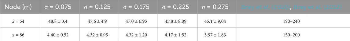
TABLE 3. Mean ± standard deviation of the computed settlements in the western (x = 54 [m]) and eastern (x = 86 [m]) nodes for different levels of V_s spatial variability (in millimeters). Reference values reported in Bray et al. (2010), Bray et al. (2012) are also included.

8 Conclusion

We performed effective stress analyses (ESSRAs) at the Los Presidentes site, which experienced liquefaction damage during the 2010 M_w 8.8 Maule Earthquake, in order to assess the effects of V_s heterogeneities on liquefaction response at the site. Using seismic interferometry methods, we identified three distinct velocity profiles consistent with the geological setting of Metropolitan Concepcion, and representative of the site conditions. Using the profile that most accurately represented free-field conditions, we generated 2D V_s heterogeneous model realizations at various levels of ${\sigma }_{ln,v_s}$ using Gaussian correlated random fields. Our simulation results demonstrate that increasing ${\sigma }_{ln,v_s}$ in near-surface soil elements, which exhibit nonlinear and liquefaction-like behavior due to earthquake-induced pore-water pressure buildup, leads to a decrease in median maximum shear, volumetric strains, and vertical settlements. We argue that when nonlinear behavior begins, an increase in damping at the element level is responsible for this reduction in the computed measurements. Furthermore, the influence of ${\sigma }_{ln,v_s}$ on the liquefaction response is more pronounced at shallow depths, where both V_s values and the confining pressure values are lower because the damping of the soil is stiffness-dependent. On the other hand, increasing ${\sigma }_{ln,v_s}$ did not significantly alter the deformation patterns of soil elements that exhibit non-liquefaction behavior. This implies that V_s influence on liquefaction triggering is minimal and that the soil’s mechanical properties and the intensity of the seismic motion are the primary factors in determining whether liquefaction is triggered or not.

In the frame of liquefaction hazard assessment, the maximum computed settlements at the 20-th and 80-th percentiles were 41 and 53 mm, respectively. This highlights a significant difference considering that our simulations were conducted without accounting for the building’s load, and that the computed maximum shear strains were relatively small $(<3\%)$. We infer that for higher amplitude ground motions and softer soil conditions, V_s variability may play an important role in the final settlements and deformations.

While our findings are within the frame of a case study of liquefaction due to a megathrust earthquake, this analysis can be extended to other tectonic and geotechnical environments. In this regard, we encourage researchers to thoroughly characterize the velocity structure of a site when conducting ESSRAs for past or expected liquefaction case studies as V_s heterogeneities, which are expected to be found in the scale of liquefaction problems, can significantly alter the dynamic response of liquefiable soils, and become a key factor for assessment.

Data availability statement

The raw data supporting the conclusions of this article will be made available by the authors, without undue reservation.

Author contributions

SN-J: Conceptualization, Data curation, Formal Analysis, Investigation, Methodology, Software, Validation, Writing–original draft. GM: Conceptualization, Resources, Supervision, Writing–review and editing. MP: Methodology, Software, Supervision, Writing–review and editing. MM: Resources, Supervision, Writing–review and editing. HS: Data curation, Investigation, Methodology, Software, Writing–review and editing. AO-C: Methodology, Writing–review and editing. RA: Resources, Supervision, Writing–review and editing.

Funding

The author(s) declare financial support was received for the research, authorship, and/or publication of this article. This work was supported within the funding programme “Open Access Publikationskosten” Deutsche Forschungsgemeinschaft (DFG, German Research Foundation) - Project Number 291075472, the Millennium Nucleus CYCLO (The Seismic Cycle Along Subduction Zones) project, the Millennium Scientific Initiative (ICM) of the Chilean Government grant NC160025, and the Chilean Scientific and Technological Development Support Fund (FONDEF) grants ID16I20157 and ID22I10032.

Acknowledgments

This work was strongly supported by the Geophysics Master’s degree program at the University of Concepción. The authors thank Dr. Robert Kayen for sharing the LiDAR picture of the Los Presidentes Site. We also thank Drs. Jose Abell, Francisco Chávez García, Christopher de la Torre, Zhijian Qiu, and Katerina Ziotopolou for providing valuable insights at different stages of this research. We very much appreciate the support of the STKO Team for providing guidance through the simulation steps with STKO-OpenSEES, and the innovative tools they developed that helped our analyses. Finally, we thank Sahiling Alarcón, Nicolás Bastías, Javier Mora and Alfonso Núñez, for their invaluable help in carrying out the field measurements. We would like to express our gratitude to the reviewers for their valuable input and constructive feedback on this research.

Conflict of interest

The authors declare that the research was conducted in the absence of any commercial or financial relationships that could be construed as a potential conflict of interest.

Publisher’s note

All claims expressed in this article are solely those of the authors and do not necessarily represent those of their affiliated organizations, or those of the publisher, the editors and the reviewers. Any product that may be evaluated in this article, or claim that may be made by its manufacturer, is not guaranteed or endorsed by the publisher.

Supplementary material

The Supplementary Material for this article can be found online at: https://www.frontiersin.org/articles/10.3389/feart.2024.1354058/full#supplementary-material

References

Aki, K. (1957). Space and time spectra of stationary stochastic waves, with special reference to microtremors. Bull. Earthq. Res. Inst. 35, 415–456.

Google Scholar

Aki, K. (1980). Attenuation of shear-waves in the lithosphere for frequencies from 0.05 to 25 Hz. Phys. Earth Planet. Interiors 21, 50–60. doi:10.1016/0031-9201(80)90019-9

CrossRef Full Text | Google Scholar

Andrus, R. D., and Stokoe, K. H. (2000). Liquefaction resistance of soils from shear-wave velocity. J. Geotechnical Geoenvironmental Eng. 126, 1015–1025. doi:10.1061/(asce)1090-0241(2000)126:11(1015)

CrossRef Full Text | Google Scholar

Assimaki, D. (2004). Topography effects in the 1999 Athens earthquake: Engineering issues in seismology. Ph.D. thesis, Massachusetts Institute of Technology.

Google Scholar

Assimaki, D., Ledezma, C., Montalva, G. A., Tassara, A., Mylonakis, G., and Boroschek, R. (2012). Site effects and damage patterns. Earthq. Spectra 28, 55–74. doi:10.1193/1.4000029

CrossRef Full Text | Google Scholar

Assimaki, D., Pecker, A., Popescu, R., and Prevost, J. (2003). Effects of spatial variability of soil properties on surface ground motion. J. Earthq. Eng. 7, 1–44. doi:10.1080/13632460309350472

CrossRef Full Text | Google Scholar

Asten, M. W., and Henstridge, J. (1984). Array estimators and the use of microseisms for reconnaissance of sedimentary basins. Geophysics 49, 1828–1837. doi:10.1190/1.1441596

CrossRef Full Text | Google Scholar

Baser, T., Nawaz, K., Chung, A., Faysal, S., and Numanoglu, O. A. (2023). Ground movement patterns and shallow foundation performance in Iskenderun coastline during the 2023 Kahramanmaras earthquake sequence. Earthq. Eng. Eng. Vib. 22, 867–881. doi:10.1007/s11803-023-2205-9

CrossRef Full Text | Google Scholar

Bassal, P. C., and Boulanger, R. W. (2021). System response of an interlayered deposit with spatially preferential liquefaction manifestations. J. Geotechnical Geoenvironmental Eng. 147, 05021013. doi:10.1061/(asce)gt.1943-5606.0002684

CrossRef Full Text | Google Scholar

Bassal, P. C., and Boulanger, R. W. (2023). System response of an interlayered deposit with a localized graben deformation in the Northridge earthquake. Soil Dyn. Earthq. Eng. 165, 107668. doi:10.1016/j.soildyn.2022.107668

CrossRef Full Text | Google Scholar

Bensen, G., Ritzwoller, M., Barmin, M., Levshin, A. L., Lin, F., Moschetti, M., et al. (2007). Processing seismic ambient noise data to obtain reliable broad-band surface wave dispersion measurements. Geophys. J. Int. 169, 1239–1260. doi:10.1111/j.1365-246x.2007.03374.x

CrossRef Full Text | Google Scholar

Biot, M. A. (1956). Theory of propagation of elastic waves in a fluid-saturated porous solid. II. Higher frequency range. J. Acoust. Soc. Am. 28, 179–191. doi:10.1121/1.1908241

CrossRef Full Text | Google Scholar

Bonnefoy-Claudet, S., Cotton, F., and Bard, P.-Y. (2006). The nature of noise wavefield and its applications for site effects studies: a literature review. Earth-Science Rev. 79, 205–227. doi:10.1016/j.earscirev.2006.07.004

CrossRef Full Text | Google Scholar

Boulanger, R. W., and Idriss, I. (2014). CPT and SPT based liquefaction triggering procedures. Report No. UCD/CGM.-14 1.

Google Scholar

Boulanger, R. W., Meyers, M. W., Mejia, L. H., and Idriss, I. M. (1998). Behavior of a fine-grained soil during the Loma Prieta earthquake. Can. Geotechnical J. 35, 146–158. doi:10.1139/t97-078

CrossRef Full Text | Google Scholar

Boulanger, R. W., and Montgomery, J. (2016). Nonlinear deformation analyses of an embankment dam on a spatially variable liquefiable deposit. Soil Dyn. Earthq. Eng. 91, 222–233. doi:10.1016/j.soildyn.2016.07.027

CrossRef Full Text | Google Scholar

Bray, J., Arduino, P., Ashford, S., Asimaki, D., Eldridge, T., Frost, J., et al. (2010). Geo-Engineering reconnaissance of the 2010 Maule. Chile Earthq. 1–347.

PubMed Abstract | Google Scholar

Bray, J., Rollins, K., Hutchinson, T., Verdugo, R., Ledezma, C., Mylonakis, G., et al. (2012). Effects of ground failure on buildings, ports, and industrial facilities. Earthq. Spectra 28, 97–118. doi:10.1193/1.4000034

CrossRef Full Text | Google Scholar

Bray, J. D., and Luque, R. (2017). Seismic performance of a building affected by moderate liquefaction during the Christchurch earthquake. Soil Dyn. Earthq. Eng. 102, 99–111. doi:10.1016/j.soildyn.2017.08.011

CrossRef Full Text | Google Scholar

Bray, J. D., and Sancio, R. B. (2006). Assessment of the liquefaction susceptibility of fine-grained soils. J. Geotechnical Geoenvironmental Eng. 132, 1165–1177. doi:10.1061/(asce)1090-0241(2006)132:9(1165)

CrossRef Full Text | Google Scholar

Campos, J., Hatzfeld, D., Madariaga, R., López, G., Kausel, E., Zollo, A., et al. (2002). A seismological study of the 1835 seismic gap in south-central Chile. Phys. Earth Planet. Interiors 132, 177–195. doi:10.1016/s0031-9201(02)00051-1

CrossRef Full Text | Google Scholar

Chávez-García, F. J., and Luzón, F. (2005). On the correlation of seismic microtremors. J. Geophys. Res. Solid Earth 110. doi:10.1029/2005jb003671

CrossRef Full Text | Google Scholar

Chávez-García, F. J., Rodríguez, M., and Stephenson, W. R. (2005). An alternative approach to the SPAC analysis of microtremors: exploiting stationarity of noise. Bull. Seismol. Soc. Am. 95, 277–293. doi:10.1785/0120030179

CrossRef Full Text | Google Scholar

Cox, B. R., and Teague, D. P. (2016). Layering ratios: a systematic approach to the inversion of surface wave data in the absence of a priori information. Geophys. J. Int. 207, 422–438. doi:10.1093/gji/ggw282

CrossRef Full Text | Google Scholar

Cubrinovski, M., Rhodes, A., Ntritsos, N., and Van Ballegooy, S. (2019). System response of liquefiable deposits. Soil Dyn. Earthq. Eng. 124, 212–229. doi:10.1016/j.soildyn.2018.05.013

CrossRef Full Text | Google Scholar

Curtis, A., Gerstoft, P., Sato, H., Snieder, R., and Wapenaar, K. (2006). Seismic interferometry—turning noise into signal. Lead. Edge 25, 1082–1092. doi:10.1190/1.2349814

CrossRef Full Text | Google Scholar

Dashti, S., and Bray, J. D. (2013). Numerical simulation of building response on liquefiable sand. J. Geotechnical Geoenvironmental Eng. 139, 1235–1249. doi:10.1061/(asce)gt.1943-5606.0000853

CrossRef Full Text | Google Scholar

de la Torre, C. A., Bradley, B. A., and McGann, C. R. (2022a). 2d Geotechnical site-response analysis including soil heterogeneity and wave scattering. Earthq. Spectra 38, 1124–1147. doi:10.1177/87552930211056667

CrossRef Full Text | Google Scholar

de la Torre, C. A., Bradley, B. A., Stewart, J. P., and McGann, C. R. (2022b). Can modeling soil heterogeneity in 2D site response analyses improve predictions at vertical array sites? Earthq. Spectra, 87552930221105107. doi:10.1177/87552930221105107

CrossRef Full Text | Google Scholar

Emergeo Working Group (2013). Liquefaction phenomena associated with the Emilia earthquake sequence of May June 2012. Available at: https://nhess.copernicus.org/articles/13/935/2013/ (Northern Italy: Natural Hazards and Earth System Sciences), 13 (4), 935–947. doi:10.5194/nhess-13-935-2013

CrossRef Full Text | Google Scholar

Ekström, G. (2014). Love and Rayleigh phase-velocity maps, 5–40 s, of the western and central USA from USArray data. Earth Planet. Sci. Lett. 402, 42–49. doi:10.1016/j.epsl.2013.11.022

CrossRef Full Text | Google Scholar

Ekström, G., Abers, G. A., and Webb, S. C. (2009). Determination of surface-wave phase velocities across USArray from noise and Aki’s spectral formulation. Geophys. Res. Lett. 36. doi:10.1029/2009gl039131

CrossRef Full Text | Google Scholar

El Haber, E., Cornou, C., Jongmans, D., Abdelmassih, D. Y., Lopez-Caballero, F., and Al-Bittar, T. (2019). Influence of 2D heterogeneous elastic soil properties on surface ground motion spatial variability. Soil Dyn. Earthq. Eng. 123, 75–90. doi:10.1016/j.soildyn.2019.04.014

CrossRef Full Text | Google Scholar

Galli, C. (1967). Geología urbana y suelo de fundación de concepción y talcahuano, Chile. Universidad de Concepción.

Google Scholar

Garofalo, F., Foti, S., Hollender, F., Bard, P., Cornou, C., Cox, B., et al. (2016). InterPACIFIC project: comparison of invasive and non-invasive methods for seismic site characterization. Part II: inter-comparison between surface-wave and borehole methods. Soil Dyn. Earthq. Eng. 82, 241–254. doi:10.1016/j.soildyn.2015.12.009

CrossRef Full Text | Google Scholar

Green, R. A., Cubrinovski, M., Cox, B., Wood, C., Wotherspoon, L., Bradley, B., et al. (2014). Select liquefaction case histories from the 2010–2011 Canterbury earthquake sequence. Earthq. Spectra 30, 131–153. doi:10.1193/030713eqs066m

CrossRef Full Text | Google Scholar

Hallal, M. M., and Cox, B. R. (2023). What spatial area influences seismic site response: insights gained from multiazimuthal 2D ground response analyses at the treasure island downhole array. J. Geotechnical Geoenvironmental Eng. 149, 04022124. doi:10.1061/jggefk.gteng-11023

CrossRef Full Text | Google Scholar

Harkrider, D. G. (1964). Surface waves in multilayered elastic media I. Rayleigh and Love waves from buried sources in a multilayered elastic half-space. Bull. Seismol. Soc. Am. 54, 627–679. doi:10.1785/bssa0540020627

CrossRef Full Text | Google Scholar

Hashash, Y. M., and Park, D. (2001). Non-linear one-dimensional seismic ground motion propagation in the Mississippi embayment. Eng. Geol. 62, 185–206. doi:10.1016/s0013-7952(01)00061-8

CrossRef Full Text | Google Scholar

Hashash, Y. M., and Park, D. (2002). Viscous damping formulation and high frequency motion propagation in non-linear site response analysis. Soil Dyn. Earthq. Eng. 22, 611–624. doi:10.1016/s0267-7261(02)00042-8

CrossRef Full Text | Google Scholar

Hu, J. (2023). Empirical relationships between earthquake magnitude and maximum distance based on the extended global liquefaction-induced damage cases. Acta Geotech. 18, 2081–2095. doi:10.1007/s11440-022-01637-y

CrossRef Full Text | Google Scholar

Huang, D., Wang, G., Du, C., and Jin, F. (2021). Seismic amplification of soil ground with spatially varying shear wave velocity using 2D spectral element method. J. Earthq. Eng. 25, 2834–2849. doi:10.1080/13632469.2019.1654946

CrossRef Full Text | Google Scholar

Hutabarat, D., and Bray, J. D. (2021). Effective stress analysis of liquefiable sites to estimate the severity of sediment ejecta. J. Geotechnical Geoenvironmental Eng. 147, 04021024. doi:10.1061/(asce)gt.1943-5606.0002503

CrossRef Full Text | Google Scholar

Inzunza, D. A., Montalva, G. A., Leyton, F., Prieto, G., and Ruiz, S. (2019). Shallow ambient-noise 3D tomography in the Concepción basin, Chile: implications for low-frequency ground motions. Bull. Seismol. Soc. Am. 109, 75–86. doi:10.1785/0120180061

CrossRef Full Text | Google Scholar

Ishihara, K. (1993). Liquefaction and flow failure during earthquakes. Geotechnique 43, 351–451. doi:10.1680/geot.1993.43.3.351

CrossRef Full Text | Google Scholar

Joyner, W. B., and Chen, A. T. (1975). Calculation of nonlinear ground response in earthquakes. Bull. Seismol. Soc. Am. 65, 1315–1336. doi:10.1785/BSSA0650051315

CrossRef Full Text | Google Scholar

Kayen, R., Moss, R., Thompson, E., Seed, R., Cetin, K., Der Kiureghian, A., et al. (2013). Shear-wave velocity–based probabilistic and deterministic assessment of seismic soil liquefaction potential. J. Geotechnical Geoenvironmental Eng. 139, 407–419. doi:10.1061/(asce)gt.1943-5606.0000743

CrossRef Full Text | Google Scholar

Khosravifar, A., Elgamal, A., Lu, J., and Li, J. (2018). A 3D model for earthquake-induced liquefaction triggering and post-liquefaction response. Soil Dyn. Earthq. Eng. 110, 43–52. doi:10.1016/j.soildyn.2018.04.008

CrossRef Full Text | Google Scholar

Kissling, E. (1988). Geotomography with local earthquake data. Rev. Geophys. 26, 659–698. doi:10.1029/rg026i004p00659

CrossRef Full Text | Google Scholar

Lobkis, O. I., and Weaver, R. L. (2001). On the emergence of the green’s function in the correlations of a diffuse field. J. Acoust. Soc. Am. 110, 3011–3017. doi:10.1121/1.1417528

CrossRef Full Text | Google Scholar

Luque, R., and Bray, J. D. (2017). Dynamic analyses of two buildings founded on liquefiable soils during the Canterbury earthquake sequence. J. Geotechnical Geoenvironmental Eng. 143, 04017067. doi:10.1061/(asce)gt.1943-5606.0001736

CrossRef Full Text | Google Scholar

Luque, R., and Bray, J. D. (2020). Dynamic soil-structure interaction analyses of two important structures affected by liquefaction during the Canterbury earthquake sequence. Soil Dyn. Earthq. Eng. 133, 106026. doi:10.1016/j.soildyn.2019.106026

CrossRef Full Text | Google Scholar

Lysmer, J., and Kuhlemeyer, R. L. (1969). Finite dynamic model for infinite media. J. Eng. Mech. Div. 95, 859–877. doi:10.1061/jmcea3.0001144

CrossRef Full Text | Google Scholar

Ma, Y., and Clayton, R. W. (2014). The crust and uppermost mantle structure of southern Peru from ambient noise and earthquake surface wave analysis. Earth Planet. Sci. Lett. 395, 61–70. doi:10.1016/j.epsl.2014.03.013

CrossRef Full Text | Google Scholar

McGann, C. R., Arduino, P., and Mackenzie-Helnwein, P. (2012). Stabilized single-point 4-node quadrilateral element for dynamic analysis of fluid saturated porous media. Acta Geotech. 7, 297–311. doi:10.1007/s11440-012-0168-5

CrossRef Full Text | Google Scholar

McKenna, F. (2011). OpenSees: a framework for earthquake engineering simulation. Comput. Sci. Eng. 13, 58–66. doi:10.1109/mcse.2011.66

CrossRef Full Text | Google Scholar

Menke, W., and Jin, G. (2015). Waveform fitting of cross spectra to determine phase velocity using Aki’s formula. Bull. Seismol. Soc. Am. 105, 1619–1627. doi:10.1785/0120140245

CrossRef Full Text | Google Scholar

Montalva, G., Ruz, F., Escribano, D., Bastías, N., Espinoza, D., and Paredes, F. (2022). Chilean liquefaction case history database. Earthq. Spectra 38, 2260–2280. doi:10.1177/87552930211070313

CrossRef Full Text | Google Scholar

Montalva, G. A., Bastías, N., and Rodriguez-Marek, A. (2017). Ground-motion prediction equation for the Chilean subduction zone. Bull. Seismol. Soc. Am. 107, 901–911. doi:10.1785/0120160221

CrossRef Full Text | Google Scholar

Montalva, G. A., Chávez-Garcia, F. J., Tassara, A., and Jara Weisser, D. M. (2016). Site effects and building damage characterization in Concepción after the Mw 8.8 Maule earthquake. Earthq. Spectra 32, 1469–1488. doi:10.1193/101514eqs158m

CrossRef Full Text | Google Scholar

Montgomery, J., and Boulanger, R. W. (2017). Effects of spatial variability on liquefaction-induced settlement and lateral spreading. J. Geotechnical Geoenvironmental Eng. 143, 04016086. doi:10.1061/(asce)gt.1943-5606.0001584

CrossRef Full Text | Google Scholar

Moreno, M., Rosenau, M., and Oncken, O. (2010). 2010 Maule earthquake slip correlates with pre-seismic locking of Andean subduction zone. Nature 467, 198–202. doi:10.1038/nature09349

PubMed Abstract | CrossRef Full Text | Google Scholar

National Academies of Sciences, E., Medicine (2016). State of the art and practice in the assessment of earthquake-induced soil liquefaction and its consequences.

Google Scholar

Nelder, J. A., and Mead, R. (1965). A simplex method for function minimization. Comput. J. 7, 308–313. doi:10.1093/comjnl/7.4.308

CrossRef Full Text | Google Scholar

Ohori, M., Nobata, A., and Wakamatsu, K. (2002). A comparison of ESAC and FK methods of estimating phase velocity using arbitrarily shaped microtremor arrays. Bull. Seismol. Soc. Am. 92, 2323–2332. doi:10.1785/0119980109

CrossRef Full Text | Google Scholar

Olivar-Castaño, A., Pilz, M., Pedreira, D., Pulgar, J., Díaz-González, A., and González-Cortina, J. M. (2020). Regional crustal imaging by inversion of multimode Rayleigh wave dispersion curves measured from seismic noise: application to the Basque-cantabrian zone (N Spain). J. Geophys. Res. Solid Earth 125, e2020JB019559. doi:10.1029/2020jb019559

CrossRef Full Text | Google Scholar

Parolai, S., Picozzi, M., Richwalski, S., and Milkereit, C. (2005). Joint inversion of phase velocity dispersion and H/V ratio curves from seismic noise recordings using a genetic algorithm, considering higher modes. Geophys. Res. Lett. 32. doi:10.1029/2004gl021115

CrossRef Full Text | Google Scholar

Parra-Colmenares, E. J. (1996). Numerical modeling of liquefaction and lateral ground deformation including cyclic mobility and dilation response in soil systems. Rensselaer Polytechnic Institute.

Google Scholar

Petracca, M., Candeloro, F., and Camata, G. (2017). STKO user manual. Pescara, Italy: ASDEA Software Technology, 551.

Google Scholar

Picozzi, M., Parolai, S., Bindi, D., and Strollo, A. (2009). Characterization of shallow geology by high-frequency seismic noise tomography. Geophys. J. Int. 176, 164–174. doi:10.1111/j.1365-246x.2008.03966.x

PubMed Abstract | CrossRef Full Text | Google Scholar

Pilz, M., and Cotton, F. (2019). Does the one-dimensional assumption hold for site response analysis? A study of seismic site responses and implication for ground motion assessment using KiK-net strong-motion data. Earthq. Spectra 35, 883–905. doi:10.1193/050718eqs113m

CrossRef Full Text | Google Scholar

Pilz, M., Cotton, F., and Zhu, C. (2021). How much are sites affected by two-and three-dimensional site effects? A study based on single-station earthquake records and implications for ground motion modelling. Geophys. J. Int. 228, 1992–2004. doi:10.1093/gji/ggab454

CrossRef Full Text | Google Scholar

Pilz, M., Parolai, S., Picozzi, M., and Bindi, D. (2012). Three-dimensional shear wave velocity imaging by ambient seismic noise tomography. Geophys. J. Int. 189, 501–512. doi:10.1111/j.1365-246x.2011.05340.x

CrossRef Full Text | Google Scholar

Pilz, M., Parolai, S., and Woith, H. (2017). A 3-D algorithm based on the combined inversion of Rayleigh and Love waves for imaging and monitoring of shallow structures. Geophys. J. Int. 209, 152–166. doi:10.1093/gji/ggx005

CrossRef Full Text | Google Scholar

Poblete, M., and Dobry, R. (1968). Modelo dinámico del suelo de concepción. Rev. IDIEM 7, 12–18.

Google Scholar

Popescu, R. (1995). Stochastic variability of soil properties: data analysis, digital simulation, effects on system behavior. Princeton University.

Google Scholar

Popescu, R., Prévost, J. H., and Deodatis, G. (1997). Effects of spatial variability on soil liquefaction: some design recommendations. Geotechnique 47, 1019–1036. doi:10.1680/geot.1997.47.5.1019

CrossRef Full Text | Google Scholar

Popescu, R., Prevost, J.-H., and Deodatis, G. (2005). 3D effects in seismic liquefaction of stochastically variable soil deposits. Geotechnique 55, 21–31. doi:10.1680/geot.2005.55.1.21

CrossRef Full Text | Google Scholar

Popescu, R., Prevost, J. H., Deodatis, G., and Chakrabortty, P. (2006). Dynamics of nonlinear porous media with applications to soil liquefaction. Soil Dyn. Earthq. Eng. 26, 648–665. doi:10.1016/j.soildyn.2006.01.015

CrossRef Full Text | Google Scholar

Pretell, R., Ziotopoulou, K., and Davis, C. A. (2021). Liquefaction and cyclic softening at balboa boulevard during the 1994 northridge earthquake. J. Geotechnical Geoenvironmental Eng. 147, 05020014. doi:10.1061/(asce)gt.1943-5606.0002417

CrossRef Full Text | Google Scholar

Qiu, Z., Prabhakaran, A., and Elgamal, A. (2023). A three-dimensional multi-surface plasticity soil model for seismically-induced liquefaction and earthquake loading applications. Acta Geotech. 18, 5123–5146. doi:10.1007/s11440-023-01941-1

CrossRef Full Text | Google Scholar

Ramirez, J., Barrero, A. R., Chen, L., Dashti, S., Ghofrani, A., Taiebat, M., et al. (2018). Site response in a layered liquefiable deposit: evaluation of different numerical tools and methodologies with centrifuge experimental results. J. Geotechnical Geoenvironmental Eng. 144, 04018073. doi:10.1061/(asce)gt.1943-5606.0001947

CrossRef Full Text | Google Scholar

Ritzwoller, M. H., Lin, F.-C., and Shen, W. (2011). Ambient noise tomography with a large seismic array. Comptes Rendus Geosci. 343, 558–570. doi:10.1016/j.crte.2011.03.007

CrossRef Full Text | Google Scholar

Ruegg, J., Rudloff, A., Vigny, C., Madariaga, R., De Chabalier, J., Campos, J., et al. (2009). Interseismic strain accumulation measured by GPS in the seismic gap between Constitución and Concepción in Chile. Phys. Earth Planet. Interiors 175, 78–85. doi:10.1016/j.pepi.2008.02.015

CrossRef Full Text | Google Scholar

Saldaña, H., Montalva, G., Escribano, D., Núñez-Jara, S., and Tiznado, J. C. (2023). Two-dimensional nonlinear dynamic analysis of a liquefaction case history considering spatial variability, and long-duration megathrust earthquakes. Soil Dyn. Earthq. Eng. (in press).

Google Scholar

Saldaña Sotelo, H. (2023). Modelamiento numérico de asentamientos inducidos por licuación en la zona subductiva chilena. Master thesis, University of Concepcion.

Google Scholar

Seed, H. B., and Idriss, I. M. (1971). Simplified procedure for evaluating soil liquefaction potential. J. Soil Mech. Found. Div. 97, 1249–1273. doi:10.1061/jsfeaq.0001662

CrossRef Full Text | Google Scholar

Shapiro, N. M., and Campillo, M. (2004). Emergence of broadband Rayleigh waves from correlations of the ambient seismic noise. Geophys. Res. Lett. 31. doi:10.1029/2004gl019491

CrossRef Full Text | Google Scholar

Shapiro, N. M., Campillo, M., Stehly, L., and Ritzwoller, M. H. (2005). High-resolution surface-wave tomography from ambient seismic noise. Science 307, 1615–1618. doi:10.1126/science.1108339

PubMed Abstract | CrossRef Full Text | Google Scholar

Taftsoglou, M., Valkaniotis, S., Papathanassiou, G., and Karantanellis, E. (2023). Satellite imagery for rapid detection of liquefaction surface manifestations: the case study of Türkiye–Syria 2023 earthquakes. Remote Sens. 15, 4190. doi:10.3390/rs15174190

CrossRef Full Text | Google Scholar

Tao, Y., and Rathje, E. (2020). Taxonomy for evaluating the site-specific applicability of one-dimensional ground response analysis. Soil Dyn. Earthq. Eng. 128, 105865. doi:10.1016/j.soildyn.2019.105865

CrossRef Full Text | Google Scholar

Thompson, E. M., Baise, L. G., Tanaka, Y., and Kayen, R. E. (2012). A taxonomy of site response complexity. Soil Dyn. Earthq. Eng. 41, 32–43. doi:10.1016/j.soildyn.2012.04.005

CrossRef Full Text | Google Scholar

Tiznado, J. C., Dashti, S., and Ledezma, C. (2021). Probabilistic predictive model for liquefaction triggering in layered sites improved with dense granular columns. J. Geotechnical Geoenvironmental Eng. 147, 04021100. doi:10.1061/(asce)gt.1943-5606.0002609

CrossRef Full Text | Google Scholar

Tokimatsu, K., Tamura, S., and Kojima, H. (1992). Effects of multiple modes on Rayleigh wave dispersion characteristics. J. geotechnical Eng. 118, 1529–1543. doi:10.1061/(asce)0733-9410(1992)118:10(1529)

CrossRef Full Text | Google Scholar

Tokimatsu, K., and Uchida, A. (1990). Correlation between liquefaction resistance and shear wave velocity. Soils Found. 30, 33–42. doi:10.3208/sandf1972.30.2_33

CrossRef Full Text | Google Scholar

Tsai, V. C., and Moschetti, M. P. (2010). An explicit relationship between time-domain noise correlation and spatial autocorrelation (SPAC) results. Geophys. J. Int. 182, 454–460. doi:10.1111/j.1365-246x.2010.04633.x

CrossRef Full Text | Google Scholar

Van Ballegooy, S., Malan, P., Lacrosse, V., Jacka, M., Cubrinovski, M., Bray, J., et al. (2014). Assessment of liquefaction-induced land damage for residential Christchurch. Earthq. Spectra 30, 31–55. doi:10.1193/031813eqs070m

CrossRef Full Text | Google Scholar

Vantassel, J. P., and Cox, B. R. (2021). SWinvert: a workflow for performing rigorous 1-D surface wave inversions. Geophys. J. Int. 224, 1141–1156. doi:10.1093/gji/ggaa426

CrossRef Full Text | Google Scholar

Verdugo, R., and González, J. (2015). Liquefaction-induced ground damages during the 2010 Chile earthquake. Soil Dyn. Earthq. Eng. 79, 280–295. doi:10.1016/j.soildyn.2015.04.016

CrossRef Full Text | Google Scholar

Vivallos, J., Ramírez, P., and Fonseca, A. (2010). Microzonificación sísmica de la ciudad de concepción, región del biobío. Serv. Nac. Geol. Minería. Carta Geol. Chile, Ser. Geol. Ambient. 12.

Google Scholar

Wapenaar, K., Slob, E., Snieder, R., and Curtis, A. (2010). Tutorial on seismic interferometry: Part 2—underlying theory and new advances. Geophysics 75, 75A211–75A227. doi:10.1190/1.3463440

CrossRef Full Text | Google Scholar

Ward, K. M., Porter, R. C., Zandt, G., Beck, S. L., Wagner, L. S., Minaya, E., et al. (2013). Ambient noise tomography across the central andes. Geophys. J. Int. 194, 1559–1573. doi:10.1093/gji/ggt166

CrossRef Full Text | Google Scholar

Weaver, R. L. (1982). On diffuse waves in solid media. J. Acoust. Soc. Am. 71, 1608–1609. doi:10.1121/1.387816

CrossRef Full Text | Google Scholar

Welch, P. (1967). The use of fast Fourier transform for the estimation of power spectra: a method based on time averaging over short, modified periodograms. IEEE Trans. audio electroacoustics 15, 70–73. doi:10.1109/tau.1967.1161901

CrossRef Full Text | Google Scholar

Xu, Y., Lebedev, S., Meier, T., Bonadio, R., and Bean, C. J. (2021). Optimized workflows for high-frequency seismic interferometry using dense arrays. Geophys. J. Int. 227, 875–897. doi:10.1093/gji/ggab260

CrossRef Full Text | Google Scholar

Yamanaka, H., and Ishida, H. (1996). Application of genetic algorithms to an inversion of surface-wave dispersion data. Bull. Seismol. Soc. Am. 86, 436–444. doi:10.1785/bssa0860020436

CrossRef Full Text | Google Scholar

Yang, Z., Elgamal, A., and Parra, E. (2003). Computational model for cyclic mobility and associated shear deformation. J. Geotechnical Geoenvironmental Eng. 129, 1119–1127. doi:10.1061/(asce)1090-0241(2003)129:12(1119)

CrossRef Full Text | Google Scholar

Youd, T. L., and Idriss, I. M. (2001). Liquefaction resistance of soils: summary report from the 1996 NCEER and 1998 NCEER/NSF workshops on evaluation of liquefaction resistance of soils. J. geotechnical geoenvironmental Eng. 127, 297–313. doi:10.1061/(asce)1090-0241(2001)127:4(297)

CrossRef Full Text | Google Scholar

Zhang, G., Robertson, P., and Brachman, R. W. (2002). Estimating liquefaction-induced ground settlements from CPT for level ground. Can. Geotechnical J. 39, 1168–1180. doi:10.1139/t02-047

CrossRef Full Text | Google Scholar

Zhang, J., and Wang, Y. (2021). An ensemble method to improve prediction of earthquake-induced soil liquefaction: a multi-dataset study. Neural Comput. Appl. 33, 1533–1546. doi:10.1007/s00521-020-05084-2

CrossRef Full Text | Google Scholar

Zhang, Y., Xie, Y., Zhang, Y., Qiu, J., and Wu, S. (2021). The adoption of deep neural network (DNN) to the prediction of soil liquefaction based on shear wave velocity. Bull. Eng. Geol. Environ. 80, 5053–5060. doi:10.1007/s10064-021-02250-1

CrossRef Full Text | Google Scholar

Zhou, Y.-G., and Chen, Y.-M. (2007). Laboratory investigation on assessing liquefaction resistance of sandy soils by shear wave velocity. J. Geotechnical Geoenvironmental Eng. 133, 959–972. doi:10.1061/(asce)1090-0241(2007)133:8(959)

CrossRef Full Text | Google Scholar

Zienkiewicz, O., and Shiomi, T. (1984). Dynamic behaviour of saturated porous media; the generalized Biot formulation and its numerical solution. Int. J. Numer. Anal. methods geomechanics 8, 71–96. doi:10.1002/nag.1610080106

CrossRef Full Text | Google Scholar