 John J. Finnigan
 Ian N. Harman1
 Dale E. Hughes
- 1CSIRO Environment, Canberra, ACT, Australia
- 2ANU Research School of Biology, Canberra, ACT, Australia
- 3ANU Fenner School of Environment and Society, Canberra, ACT, Australia
It has long been suspected that thermo-topographic flows, especially gravity currents, within vegetation canopies on complex terrain are one of the main reasons behind the failure to reconcile micrometeorological and biometric estimates of canopy-atmosphere exchange at many sites. However, the physical mechanisms governing the initiation and the scaling of these flows remain poorly understood. Here we present the results of a novel wind tunnel study that looks in detail at the flow within and above an open canopy in stably stratified conditions and investigates the physical mechanisms responsible for gravity currents within canopies. The wind tunnel simulations demonstrate that gravity currents are established through a complex balance of competing forces on the flow within the canopy. Three forcing terms act on the flow in the canopy as it passes over the hill. First is the hydrodynamic pressure gradient associated with the boundary layer flow aloft; second, a hydrostatic pressure gradient associated with the displacement of temperature and density surfaces by the hill, and finally a thermal wind term, where a streamwise pressure gradient is caused by changes in the depth of the temperature perturbations to the flow. The net balance of these forces is opposed by the canopy drag. Gravity currents, however, do not appear unless the turbulence, which supports the transport of momentum into the canopy, is also reduced. This suppression occurs preferentially deep within the canopy due to a Richardson number cut-off effect, which is directly linked to the different transport mechanisms of heat and momentum across the boundary layers on the canopy elements. The gravity current first appears at the ground surface, despite cooling profiles that are concentrated in the upper canopy. Once initiated, a gravity current can propagate substantial distances away from the triggering topography, driven by the thermal wind term. If shown to be robust these results have widespread implications for the micrometeorology, atmospheric boundary layer and numerical weather prediction communities.
1 Introduction
Flow in the atmospheric boundary layer continually adjusts as it passes over the landscape with associated impacts on the exchange of mass and energy with the surface. At least in landscapes comprised of rough surfaces on gentle topography there is now a good understanding of the impacts on the flow and turbulence (e.g., Hunt et al., 1988a; Hunt et al., 1988b) and on the scalar fields and fluxes (e.g., Raupach et al., 1992; Raupach and Finnigan, 1997; Huntingford et al., 1998). However, our understanding of the impacts when the topography is covered by a plant canopy is far less complete (e.g., Lee, 2000; Finnigan et al., 2020).
As well as the impact of topography on the boundary layer itself, one application where its effects are critical is the measurement of the exchange of biologically important scalars between the surface and atmosphere using eddy flux towers, especially within the FLUXNET community (Baldocchi et al., 2000; Baldocchi et al., 2001; https://fluxnet.org). For practical reasons many FLUXNET sites are located in regions of complex topography and over tall canopies, and by design must operate in most synoptic conditions. The FLUXNET community has long suspected, and repeatedly confirmed, that the combination of a canopy, radiative cooling and topography can lead to the formation of thermo-topographic flows within the canopy, which can be decoupled from the flow above, even though this can remain turbulent (e.g. Staebler and Fitzjarrald, 2004; Froelich and Schmid, 2006; Goulden et al., 2006, van Gorsel et al., 2008). This is a serious problem because the eddy flux methodology relies on the turbulent coupling and rapid mixing of the air layers between the surface and the sensor locations.
Thermo-topographic flows also lead to advective fluxes, which cannot be measured from single towers. This can result in failure to close the energy balance and overestimation of diurnal carbon exchange because night-time respiration from soil and canopy is not measured at the flux instrument (e.g., Aubinet et al., 2005; Goulden et al., 2006; Foken et al., 2006). The issue is ubiquitous, and it is now routine to apply a filtering technique (e.g., the u* threshold) to remove and replace suspect episodes from the observations (Falge et al., 2001; Gu et al., 2005). However, such filtering techniques remain largely site specific and for some sites can lead to the removal of all data (e.g., van Gorsel et al., 2007). Methods to overcome the issue by direct measurements, for example, using multiple towers (Feigenwinter et al., 2008), measuring the fluxes across all sides of a control volume (Leuning et al., 2008), statistical interpolation (van Gorsel et al., 2007; van Gorsel et al., 2008) or the combination of tower and ancillary measurements using machine learning (e.g., Barzca et al., 2009; Emanuel et al., 2011; Metzger, 2018; Xu et al., 2018; Chi et al., 2019) are under continual development but are themselves faced with difficulties associated with observational techniques or site to site variability.
There has been a range of attempts to obtain detailed knowledge of the mechanisms responsible for thermo-topographic flows and how these relate to the easily observable features of a site, such as hill shape, canopy height and leaf area distribution. These have been comprehensively reviewed in Finnigan et al. (2020) and include directly relevant studies such as the field observations of van Gorsel et al. (2003) made as part of the large MAP-RIVIERA study of hill and valley flows (Rotach et al., 2004), the laboratory simulations of a turbulent gravity current through a canopy of obstacles in a flume by Hatcher et al. (2000) and the numerical modelling of Watanabe (1994), who studied the initiation of a gravity current in a canopy by radiative cooling. Analytic and numerical modelling of flow in canopies on hills has advanced considerably in the last two decades (e.g., Finnigan and Belcher, 2004; Ross and Vosper, 2005; Katul et al., 2006; Patton et al., 2006; Belcher et al., 2008; Harman and Finnigan, 2010; Belcher et al., 2012; Harman and Finnigan, 2013) explicitly included stability influences in extensions of earlier analytic models. What all these studies indicate, is that the presence of a deep canopy amplifies the effects of diabatic stability and promotes the development of gravity currents, but the model studies generally lack experimental validation, which has not yet been done in a systematic way.
Here we attempt to address this problem through some novel wind tunnel experiments. We investigate the flow past a gentle isolated 2-dimensional ridge, covered by a canopy, in neutrally and stably stratified conditions. Scale experiments can provide the controlled conditions required to obtain the repeatable and robust observations needed to understand the physical processes involved in any particular circumstance. They have been widely used in the field of boundary layer flow over hills (Finnigan et al., 1990; Ayotte and Hughes, 2003 and references therein), including in the case of neutrally stratified flow over hills covered with canopies (Finnigan and Brunet, 1995; Poggi and Katul, 2007a; Poggi and Katul, 2007b; Poggi et al., 2007; Harman and Finnigan, 2013).
While the FLUXNET problem provides the immediate motivation for these experiments, they also fill an important gap in our understanding of boundary layer flow in complex topography more generally, a field which has been comprehensively reviewed recently by Finnigan et al. (2020). Among many applications, better understanding is critical for the continued development of high-resolution numerical weather prediction, the representation of the surface energy balance and carbon cycle components within Earth system models, wind farm siting and yield predictions and the measurement and modelling of the long-distance transport of trace gases.
This paper is structured as follows: First we give a brief description of the underlying framework, through which we will analyse the results and then we describe the experimental configuration. Section 3 introduces the neutrally stratified reference case and tests whether we are able to simulate turbulent flow at low wind speeds, a necessary precursor for the stably stratified experiment. Section 4 then considers the behaviour of the flow as the wind speed is reduced, a stable layer is generated at the surface, and the gravity current is initiated. Section 5 describes some key characteristics of the resulting gravity current and section 6 looks more closely at its dynamics. We conclude with a general discussion and place these results in the context of full-scale flow.
2 Flow over a gentle ridge in stably stratified conditions
We consider the flow over a 2D hill aligned normally to the mean flow. The model hill is an isolated sinusoidal ridge where the hill surface, zs, given by
for
Where H is the hill height and L its half length. A hill can be considered gentle if H<<L.
The flow over topography is naturally analysed in a displaced co-ordinate system (X, Z) that follows the topography close to the surface but relaxes with height towards the conventional rectangular Cartesian co-ordinate system (x,z), where x is along and z normal to constant geopotential surfaces (Belcher, 1990; Belcher et al., 1993). A suitable choice for the lines of constant Z are the streamlines of inviscid, non-rotating flow over the hill forced by a uniform wind of unit magnitude. The streamwise coordinate X is then defined so that the coordinate system is orthogonal. Hence the displaced coordinate system is given by,
for -2L>x>2L and equivalent to (x,z) outside of this range so that the origin of X and x coordinates is the hill crest.
A distinguishing attribute of a canopy, as opposed to a rough surface, is its ability to absorb momentum from the wind over an extended height range. In real canopies, the aerodynamic drag force exerted by the foliage is a mixture of pressure or ‘form’ drag and viscous drag but at the Reynolds numbers typical of real canopies, most of the drag is form drag and varies as the square of the local wind vector (Hoerner, 1965). Recognising this, our modelled canopy consists of bluff elements, practically all of whose drag is pressure drag. The canopy can therefore be characterised by an adjustment length scale, Lc (Finnigan and Brunet, 1995; Belcher et al., 2003; Belcher et al., 2008) and the (local) drag on the atmosphere is given by
2.1 Governing equations
We can partition any variable property of the flow,
where x is the position vector, the overbar represents the spatial and time average and primes the deviations from that average.
The steady state equations for the mean streamwise (5a) and cross stream (5b) components of the flow in the displaced co-ordinate system given by Eqs 2, 3 form the basis of our analysis. These equations are derived in more detail in Supplementary Appendix S1,
I. II III IV V VI VII
R is the local radius of curvature of the X coordinate lines and can be expressed in terms of the stream functions and potential functions that define the coordinates (Finnigan, 1983).
The potential temperature deficit,
There are three pressure forcing terms in Eqs 5a, 5b. Term III is the hydrodynamic pressure gradient and is established by the response of the atmosphere well above the surface to the topography. For gentle hills,
and h(X) is the height at which
The other terms in Eqs 5a, 5b represent the canopy kinematic drag (VII), the divergence of the turbulent stresses (VI) and the inertial acceleration (terms I and II respectively). The relative importance of I and II depends on the ratio of the hill length to the canopy adjustment length,
2.2 Experimental configuration
The experiments were performed in the CSIRO Pye Laboratory wind tunnel, an open return blower-type wind tunnel designed to simulate the flow in the atmospheric boundary layer (Finnigan et al., 1990). This facility has been used extensively to study the boundary layer flow over a variety of surface types, including over topography (Finnigan, 1988; Finnigan and Brunet, 1995; Ayotte and Hughes, 2003). The experimental section of the tunnel is 17 m long, 1.78 m wide and approximately 0.7 m high. The height of the tunnel roof is adjustable so that the streamwise pressure variations associated with the growth of the turbulent boundary layer can be minimized.
Experimentally it is easier to heat a surface than to cool it; by mounting the surface on the roof the (positive) buoyancy effects from heating then act in an analogous manner to (negative) buoyancy effects due to cooling in the real world once the vertical co-ordinate is reversed and temperature excesses are treated as temperature deficits.
The experiment is configured in seven sections, as shown schematically in Figure 1 (not to scale):
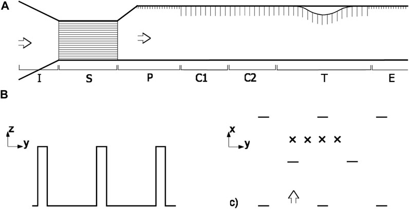
FIGURE 1. (A) Schematic of the experiment configuration used in the FC Pye Lab wind tunnel (not to scale). Labels indicate sections of the tunnel as introduced in the text: I, inflow section; S, suppression section; P, pegged section; C1, unheated canopy section; C2, heated canopy section; T, test section; and E, exit section. (B) Cross section of the canopy elements used, and (C) plan view of the element layout, with approximate measurement locations marked by “×”.
I Inflow section.
S Suppression section: used to minimise external influences on the flow and turbulence generated.
P 2 m of a rough, peg surface with an initial rapid increase in tunnel depth to trigger and generate a rough wall boundary layer.
C1 3 m of the canopy surface; used to generate an equilibrium canopy boundary layer.
C2 1.05 m of heated floor and canopy surface to generate the thermal boundary layer upwind of the hill.
T Test Section, 0.5 m of flat canopy surface followed by a 1.1 m long sinusoidal hill covered by the canopy then a further 0.5 m of flat canopy surface. The floor and canopy elements of the C2 and test sections can be heated independently.
E 1.2∼m of rough, peg surface.
The canopy elements and surface are constructed from copper plated circuit board material and painted black to enable efficient energy transfer from the element to the air and to provide contrast for flow visualisation. The elements are 60 mm high, 10 mm wide, separated by 45 mm in the streamwise direction, by 50 mm in the spanwise direction and configured in a staggered array as shown in Figure 1C. Heat is applied to the boundary layer by passing electricity through surface and canopy elements. The canopy elements are configured with their conducting copper surfaces varying with height so that approximately (2/3) of the heat energy transferred to the air from the canopy elements occurs between hc>Z>hc/2. Unless indicated otherwise, the experiments are conducted with a heating rate of 200 W m-2 partitioned equally between the ground and canopy elements. This is designed so that the canopy will act in a similar manner to an open natural canopy where radiative cooling is predominantly from the canopy crown, but some also occurs from the ground surface.
The model hill height is H=50 mm and its half-length is L=255 mm. Estimates of the adjustment length for the canopy show that Lc is approximately 240 mm. This implies that the canopy is deep enough that shear stress at the ground does not play a significant role in the dynamics of the flow. Since H/L∼0.2, the hill cannot formally be considered as gentle topography. Furthermore, as Lc/L∼1, the streamwise advection term I, will not be negligible in the canopy. Together these conditions imply that linear perturbation theories for the flow over topography (Hunt et al., 1988a) and the extensions for a canopy and stable stratification (Hunt et al., 1988b; Belcher et al., 2008) do not strictly apply and that we also need to use the extensions to Finnigan and Belcher (2004), described in Harman and Finnigan (2010, 2013), to accommodate advection in the canopy. Nevertheless, the results from these analyses still form a useful basis for the interpretation of the simulated flow.
Fast response wind measurements were made using a TSI Laser Doppler Velocimeter (LDV). Mean and turbulent air temperatures were measured with a fine wire type T thermocouple with its junction located just outside the laser beam focus. These instruments were mounted on a traversing apparatus, which provided repeatable and accurate sensor positioning. Element and floor temperatures were measured with in situ thermistors and also with an Agema imaging infra-red camera. Observations were taken over a height range of 0.1hc<Z<.4.5hc and at many streamwise locations; only a subset of the observations taken are shown, as described in the text. At each measurement location the mean and turbulent statistics were established using Reynolds decomposition. Profile measurements were taken at four lateral positions in the array, as marked by × in Figure1C), and then averaged to give a surrogate for a true spatial average (Harman Ian et al., 2016). For each experiment, and after changes in the position of the traverse apparatus, the wind tunnel flow and temperature were allowed to achieve a steady state prior to the measurements being taken. In the remainder of this paper, we will describe the experiments and observations as though the hill were the ‘right way up’ and the surface cooled.
3 Neutrally stratified flow over the hill
The aim of these experiments is to recreate real world conditions where the flow can be turbulent but stratified by cooling from below. Two dimensionless groups determine the flow characteristics: the Reynolds number,
We require the Reynolds number to be sufficiently large that the flow is fully turbulent but that the Froude number be of order 1 so that inertial and buoyancy forces are comparable. At the scale of the experiment, it is impractical to reduce the Froude number by simply increasing N0 because the temperatures required would be too high so we must also reduce U0. However, in doing so, we must ensure that, when operating the tunnel at low wind speeds, the Reynolds number remains large enough that viscous effects remain unimportant, and the flow is fully turbulent.
An analysis, given in Supplementary Appendix S2, shows that to produce flows with
Figures 2, 3 show the (spatially averaged) profiles of the mean wind vector and second moment statistics, respectively. The agreement between the high wind speed and low wind speed cases in most of the plots is good and there is no evidence that the turbulent nature of the flow is systematically suppressed at the low wind speeds. The poorest agreement is in Figure 2B and the velocity perturbation profiles are by far the noisiest of the set of results. The perturbation profiles in the canopy at X=−2L +L, +2L are good matches but the low speed curves at -L and +4L are slightly lower than the high. The discrepancies above the canopy are larger and seem quite random, which is why we believe this is largely a problem of measurement noise given that the errors associated with experimental accuracy are fractionally greater at lower wind speeds. In the profiles of the turbulent shear and normal stresses shown in Figures 3A–C we see that at some stations the high speed stresses above the canopy are slightly lower than the low speed but it is difficult to detect a systematic trend.
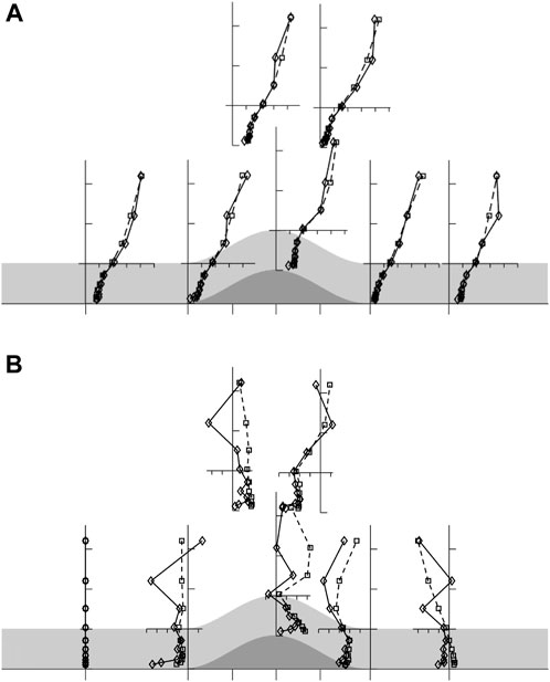
FIGURE 2. Normalized profiles of (A) total U and (B) wind speed perturbation, U-U0, with position across the hill. Profiles normalised by free stream wind speed, U0 in (A), and by U0 H/L in (B). Ticks on the horizontal axes mark every 0.2. Squares and dashed line: high wind speed case, where U0=10 ms−1. Diamonds and solid line: low wind speed case where U0=0.35 ms−1. The mean flow is from left to right. Note that while U is rotated into the (X, Z) coordinate system, the points are plotted on the vertical, x=constant, trajectories of the traverse mechanism.
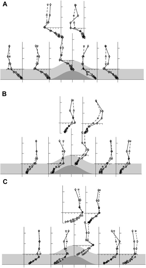
FIGURE 3. Normalized profile of turbulent statistics with position across the hill. (A)
Despite the caveats on hill steepness expressed above, it is instructive to compare these observations to the profiles predicted by linear perturbation theory. The analysis of Finnigan and Belcher (2004) involved a number of simplifying steps and assumptions, which were noted by Poggi et al. (2008) and later reviewed in some detail by Belcher et al. (2012). For the purposes of comparison with the present data, two assumptions are critical; both relate to the scale analysis that led Finnigan and Belcher (2004) to neglect the advection terms in the upper canopy flow. The assumptions were that Lc/L<<1, which is necessary if within-canopy advection is to be ignored, and that the vertical velocity induced by flow perturbations be small. This second condition can be expressed, as,
Where
In comparing with linear theory we concentrate on Figure 2B, which shows the profiles of the perturbation to the mean wind speed, defined as differences from the undisturbed upwind profile U0 (Z) measured at X=−4L; here it is appropriate to concentrate solely on the high wind speed case (dashed lines). This shows that perturbations to the flow vary in a different manner above and within the canopy. The flow perturbations above the canopy reach a maximum between X=-L and X=L. The perturbations within the canopy are positive between X=-L and X=0 and with an indication of negative flow between X=L and X=2L. This tendency is consistent with a downstream shift of the perturbation pattern as is predicted by linear perturbation theory. Such a downstream shift was also seen in the low density, narrow hill
Overall, Figures 2, 3 and the comparison with the latest linear theory demonstrate that we can simulate neutrally stratified flow over a hill and maintain dynamic similarity over a range of free stream wind speeds spanning at least 0.35–10 m s−1. Therefore, we have confidence that any changes observed in the flow when the surface is cooled arise from the impacts of that cooling and are not an effect of the reduced Reynolds Number.
4 Genesis of the gravity current
We now turn our attention to the genesis of the gravity current as the flow becomes increasingly stably stratified, i.e., as the Froude number FL is decreased. The equations of motion (5a,b) indicate that a complex balance of forces determines the flow within the canopy. However, a gravity current will only be formed on the upstream side of the hill if the hydrostatic pressure gradient term, IV exceeds those acting to accelerate the wind up the hill, i.e., the flow inertia, terms I and II, the hydrodynamic pressure gradient, III and the shear stress divergence VI. We can expect this to occur first where
Figure 4 shows profiles of the mean temperature deficit (A–C), mean wind speed (D–F) and turbulent shear stress (G–I) through the canopy and boundary layer for eight cases. In each case, 200 Wm−2 of electrical energy is applied, split equally between the surface and canopy. For presentational purposes the normalised profiles have been split into three regimes according to flow type, which we will term the turbulent (left column), transitional (centre column) and gravity current (right column) regimes.
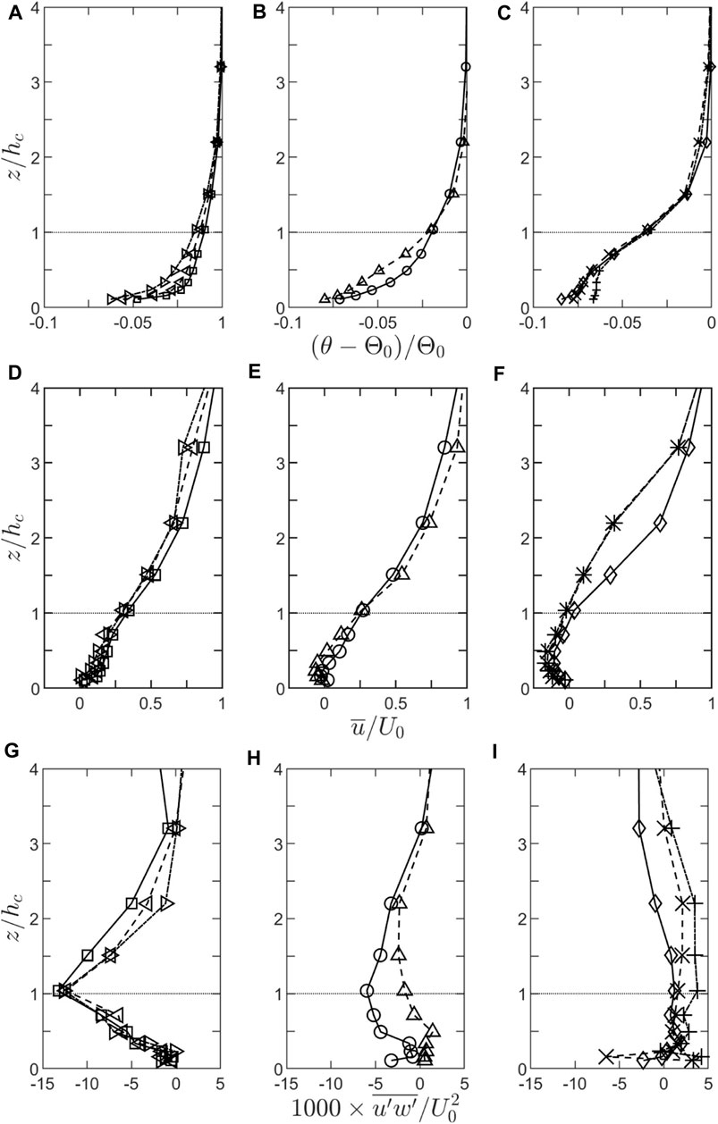
FIGURE 4. Variation of the mean temperature (A–C), mean wind speed (D–F) and turbulent shear stress (G–I) at X=-L as the free stream wind speed is reduced with the ground and canopy cooled. The profiles are plotted according to regime as described in the text. Free stream wind speeds, U0, for the various cases are: Left column, turbulent regime: triangle 0.7 m s−1, left pointing triangle 0.65 m s−1, right pointing triangle 0.6 m s−1; centre column, transition regime: circles 0.55 m s−1, triangles 0.45 m s−1; right column, gravity current regime: diamonds 0.35 m s−1, × 0.25 m s−1, +0.2 m s−1.
The wind and shear stress profiles in the turbulent regime are very similar to those in neutral conditions (Figures 2, 3) although there are some changes in the shear stress profile at X=-L. As U0 is decreased, there is also a suggestion of a decrease in flow strength in the canopy very close to the ground, which would be indicative of the start of a gravity flow, but the overall flow remains positive (uphill). The associated temperature profiles show the expected stable profile, with a strong gradient near the surface due to the restricted scales of turbulent motion and the surface cooling.
In contrast, in the gravity current regime, reversed flow is established through nearly the full depth of the canopy. The shear stress within the canopy has collapsed so there is almost no transfer of streamwise momentum from the flow above to that within the canopy. In this sense, the canopy is decoupled from the boundary layer. The temperature deficit in the flow increases through the canopy (up to around 2.0 hc), and especially in the upper canopy, as the Froude number decreases. Interestingly, there appears to be a further break in regime type when the flow becomes very stable (U0 ∼0.2 m s−1) as the temperature deficit profile becomes more uniform with height in the canopy.
However, it is the transition regime profiles which provide the most insight into the dynamics. Here the temperature profiles are very similar in character to those in the turbulent regime. There is a clearly discernible reversed (gravity) flow at the ground (deepening with decreasing FL) yet the (normalised) wind speed at canopy top is only slightly smaller than in the turbulent regime. The turbulent stress, however, is decreased in magnitude through the full depth of the profile and, in the layer with reverse flow, it is very small or zero.
To interpret these observations, we use insights from the phenomenological model for scalar and momentum transport in canopies on level terrain from Finnigan (2006), which is developed further in Belcher et al. (2008). While the details of its source/sink distribution differ from the present experiment, this model is grounded in the fundamental difference in character of the mechanisms which transport scalars and momentum to and from the canopy elements. Momentum can be exchanged at the surface of the canopy elements by both pressure forces and molecular diffusion whereas scalars are exchanged solely by molecular diffusion. The relative efficiencies of momentum and scalar transport to and from canopy elements can be expressed by comparing the adjustment length scales for momentum and scalars in the canopy.
We recall from Eq. (5a) that we express the momentum sink strength or canopy drag, D as,
A direct consequence of this is that, as we descend into a canopy cooling radiatively at night, the leaf-air temperature difference
Our experimental configuration simulates a relatively open canopy rather than a ‘closed’ canopy with a dense upper story and open trunk space so we do not observe a distinct temperature inversion in the lower canopy although at a few streamwise positions there is a weak inversion between 0.3hc>Z>0. Closed canopies with an open lower canopy or trunk space usually do demonstrate an inversion and the temperature there can be ‘well mixed’ by unstable convection from the radiatively cooling crown above. However, this well-mixed layer is still cooler than the free air away from the hill at the same geopotential level so that the gravity current will initiate in this lower open layer although the locus of cooling is the canopy top.
The Ri mechanism described above explains both the initiation of the gravity current at the ground in open canopies or in the lower canopy layer in closed canopies as well as the coincidence of that layer of reversed flow with the layer of zero-momentum flux, even though the cooling is predominately in the upper canopy. The generality of the underlying cause also suggests that these are universal features of such flows. The fact that reversed flow is generated first near the ground surface is of critical importance to the FLUXNET community as it could imply that the soil respiration term will be preferentially missed from the observation systems.
There is an important corollary to these observations and this interpretation. The suppression of momentum transfer to the canopy leads to a reduction in the volume of the canopy that is actively providing drag on the boundary layer above. Consequently, the surface then provides less drag than would otherwise be expected given the reduced wind speed, even on level terrain. This effect could be quite substantial, implying that the roughness length of canopies varies significantly with stability (see Harman and Finnigan, 2007; Harman and Finnigan, 2008). This feature, and the underlying physics, are not incorporated in the classic rough wall boundary layer Monin-Obukhov similarity formulae (e.g., Hogstrom, 1996), which are used widely in numerical weather prediction and general circulation models.
5 Characteristics of the gravity current
In this section we compare both neutral and stably stratified flow at a free stream wind speed of U0=0.35 m s−1. Section 4 shows that at this windspeed, cooling establishes a gravity current which, on the upwind slope, fills most of the canopy.
Figures 5, 6 show the profiles of mean wind speed and turbulent normal and shear stresses for the two experiments over an extended streamwise range. Also indicated on the figures are the locations of the C1:C2 and C2: T transitions (see Section 2 and Figure 1). The dominant feature in the figures is, as expected, the gravity current that is established within the canopy when canopy and surface are cooled. However, more surprising is a) the upwind extent of the reverse flow (some 2.7 m or 10.5L) and b) the relative absence of the gravity current downstream of the hill. The upwind penetration of the gravity current is remarkable and extends a distance 2L past the C1:C2 junction at X=−8.1L where the surface and canopy cooling stops. A more subtle, but equally important, feature in the flow is the acceleration of the flow above the canopy prior to the ridge crest in the boundary layer overlying the gravity current. This acceleration is significantly larger than that expected from solid and wake blockage in the wind tunnel, which is calculated to be less than 10%. Instead it is an indication of the reduction in drag applied to the boundary layer by the canopy as a result of the suppression of turbulence within the gravity current.
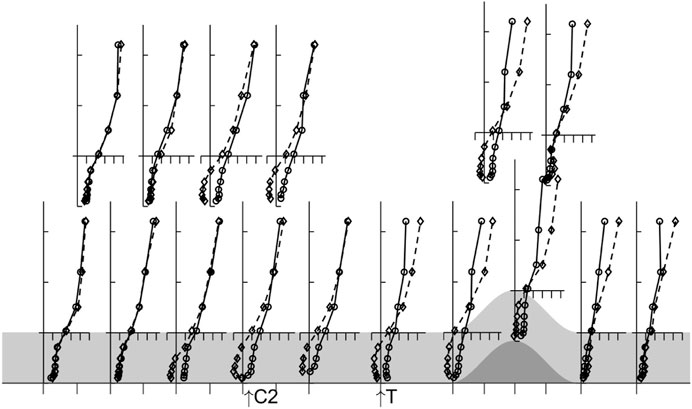
FIGURE 5. Profiles of normalised wind speed
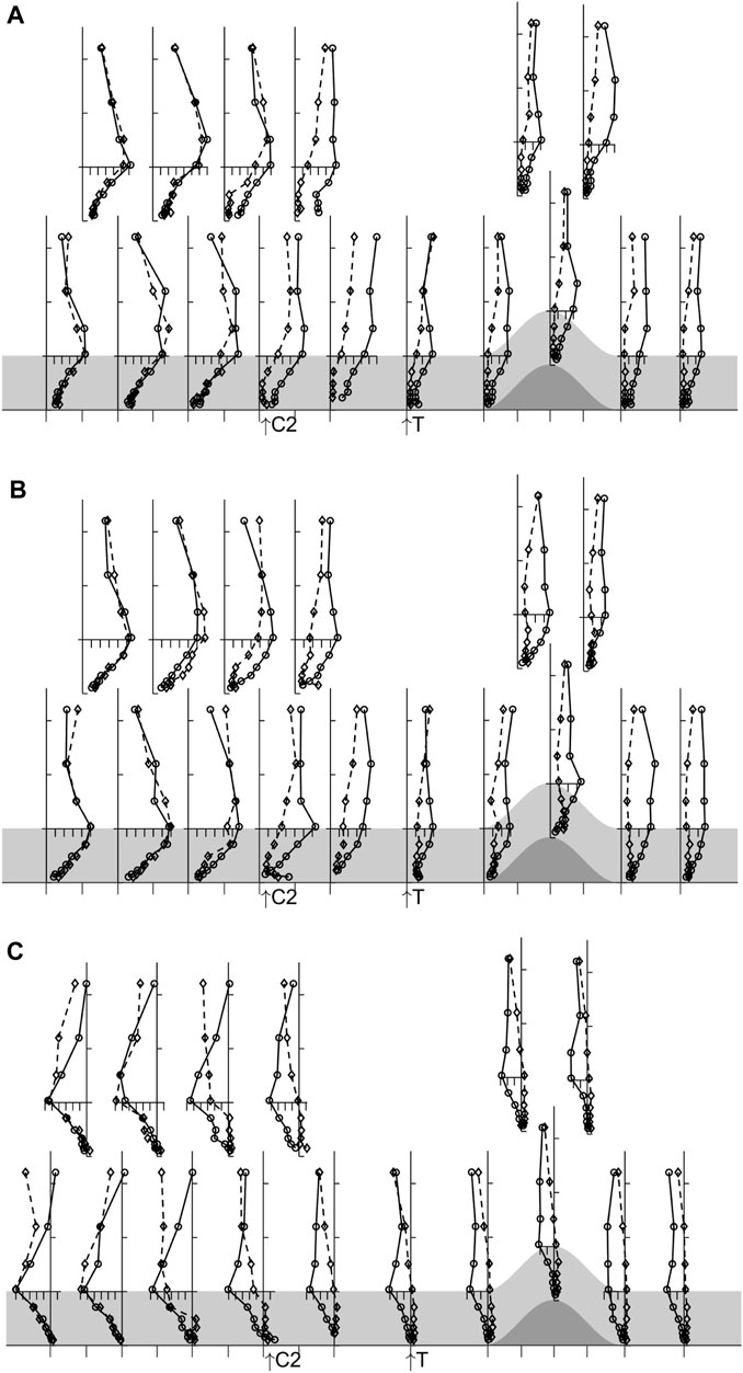
FIGURE 6. Normalised profiles of turbulent stresses, (A)
This suppression of turbulence leads to the flow in the canopy decoupling from that above in the following sense. We see in Figures 6A, B that the streamwise and cross stream velocity fluctuations, especially within the canopy but also up to Z∼3hc, are much smaller when the canopy is cooled compared to no cooling. At the same time, the shear stress falls to close to zero in the cooled canopy so little or no streamwise momentum flux is transferred into the gravity current from above. The existence of
In Figure 7 we show the profiles of temperature deficit,

FIGURE 7. Profiles of the temperature deficit
It is useful to discuss the dynamics of the gravity current using some integral measures. Recalling the definitions in section (2.1), we define the vertically integrated velocity deficit,
Comparison with Eq. 6 shows that.
Figures 8A,B show how these four measures vary with streamwise position. Difficulties with the temperature measurements at three locations,
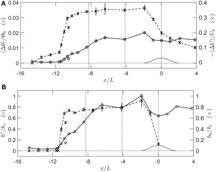
FIGURE 8. Integral measures of the gravity current. (A) o, normalised temperature deficit
First, we see in Figure 8A that the velocity deficit is roughly twice as large on the upwind side of the hill as the downwind. This should be expected given the definition of
This thinning over the hill crest is predicted by the analytic model of scalar transport over a canopy covered hill presented by Finnigan (2006). This model extends the treatment of scalar transport over a rough hill by Raupach et al. (1992) by replacing the lowest layer in Raupach et al.’s model by a two-layer canopy just as Finnigan and Belcher (2004) extended the rough hill flow model of Hunt et al. (1988a) by replacing its inner surface layer by a canopy. Finnigan’s (2006) model is restricted to neutral conditions, but its general predictions are still relevant to the present stable case. It shows that two mechanisms impact the depth and magnitude of the cool layer over the crest. First and most importantly, as the flow accelerates over the hill, inviscid effects in the model outer layer bring streamlines and isotherms closer to the surface, reducing h*. The second mechanism, which dominates in the canopy, involves changes in the source term for heat, which acts to cool the air, and which is proportional to
6 Dynamics of the gravity current
As discussed in Section 2.1, the canopy flow represents a balance between all the terms in the streamwise momentum Eq. 5a but, once flow in the canopy has decoupled from that above, the only forcing terms are the hydrodynamic and buoyancy-related pressure gradients. Since the drag force always opposes the flow, it is these forcing terms that determine the magnitude and direction of the gravity current, with the inertial terms on the left-hand side of Eq.# 5a, reflecting any imbalance between forcing and drag. In Figure 9 we follow the evolution of these forcing and response terms, integrated over the depth of the gravity current, h0 as we traverse the hill.
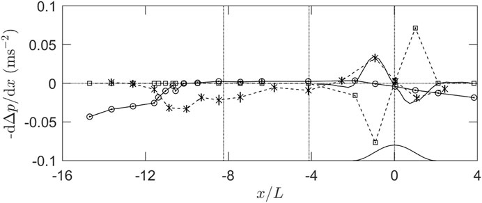
FIGURE 9. Evolution of the streamwise momentum balance. Solid line is the hydrodynamic pressure gradient; x is thermal wind term (vertical lines through the points are estimates of the uncertainty in the estimates of all terms), squares are the hydrostatic pressure gradient; o, the aerodynamic drag term. All terms are integrated over the momentum depth of the gravity current, h0.
The hydrodynamic pressure gradient was not measured directly in the experiment but has been estimated by referring to two relevant data sets. The first is a Large Eddy Simulation (LES) of the neutrally stratified flow over a very similar canopy-ridge combination performed by Dr E. G. Patton, to whom the authors are indebted. The LES pressure field shows that
The second data set was the calculation of hydrodynamic and hydrostatic pressure gradients over a sinusoidal ridge performed by Belcher et al. (2008). They took the canopy-on-hill model of Finnigan and Belcher (2004) and added the effects of a stably stratified background flow by the following procedure. They assumed that the background temperature field
Two things are relevant from their results (see Belcher et al., 2008; Figure 10). The first is the strong dependence of both the shape and magnitude of the hydrodynamic pressure gradient
In the momentum balance illustrated in Figure 9, therefore, we have chosen to use an appropriately scaled version of Patton’s LES calculation of
As already noted, over the whole streamwise extent of the gravity current, the turbulent shear stress is suppressed by the stable stratification in the canopy so that the flow is entirely determined by the pressure gradients, the canopy drag and flow inertia. On the upwind hill slope the largest single forcing term is the hydrostatic pressure gradient and this is opposed by the hydrodynamic gradient as expected, but surprisingly, also by the thermal wind term. Reference to Figures 7A,B shows that we should expect this because of the sharp increase in the depth of the thermal deficit layer between X=0 and X=−2L. We see a corresponding situation on the lee slope where the weaker hydrostatic gradient is opposed by both the hydrodynamic and thermal wind terms, which is why we do not observe net downslope flow there. Moving off the hill slope, the hydrodynamic and hydrostatic terms are zero by X=−3L and the only forcing term driving flow upwind is the thermal wind.
Between X=−2L and X=−6L, the thermal wind is approximately constant as the thermal deficit layer decreases roughly linearly upwind from its ‘hump’ at X=−2L (Figures 8A,B). From -6L to −11L, however, it increases in strength because of the stronger decrease in thermal deficit and h* corresponding to the growth of the internal boundary layer of temperature deficit. As noted in Section 5 above, this is really an artefact of the experimental configuration. Until the thermal wind ends around X=−11.5L, it is opposed primarily by the canopy drag, the calculated streamwise inertial term,
The applicability of our results to the real world depends upon the degree to which they were preconditioned by the experimental configuration. The thermal wind term in our experiments, is established through two processes. The first is the (small) turbulent mixing across the top of the drainage current, which gradually erodes the thermal deficit as the current progresses upstream. This is a general feature of gravity currents (e.g., Princevac et al., 2005). The second, which dominates between X=−6L and X=−11.5L is caused by the relatively rapid growth of the thermal internal boundary layer, which is initiated at the upstream penetration point of the cool gravity current. If the surface cooling in the wind tunnel had extended much further upwind so that the thermal layer could equilibrate well ahead of the hill, the experiment would be a better representation of natural conditions, as we expect radiative cooling of a real canopy to be spatially uniform. Hence, although the dynamics of the gravity current upwind of X=−6L, and especially its penetration well past the point at which cooling stops, is interesting and informative, we will assume that the behaviour of the stable layer between X=−6L and X=4L is more representative of conditions encountered routinely in the field. In particular, the hump in thermal layer thickness, just upwind of the hill, its thinning over the hill crest and growth on the downwind slope and the attendant behaviour of the thermal wind term is based on solid theory and seems likely to be manifested as long as the overall flow has a FL > 1.
Over the hill then, we see a competition between three forcing terms in the canopy layer. The hydrodynamic pressure gradient acts to drive the flow towards the hill crest on both upwind and downwind hill slopes but a small but significant region of adverse
Our analysis allows us to make some scaling arguments that are illuminating. First, our experiments are all at steady state, so it is necessary to ask if this is relevant to the dynamics of natural gravity currents. If the background wind is near zero so the flow that develops is entirely buoyancy driven, we can follow Hatcher et al. (2000) and estimate tc, the time to steady state by assuming that at times t << tc, the hydrostatic forcing is balanced by flow acceleration so
Inserting values typical of a deciduous forest FLUXNET site into Eq. 11 (van Gorsel et al., 2007), we find that
Since the gravity current is initiated when the downslope hydrostatic pressure gradient exceeds the hydrodynamic gradient, which is forcing the flow towards the hill crest, we can use their ratio as an indication of the possibility of a gravity current forming. Taking the hydrodynamic pressure scaling from the small perturbation analysis of flow over hills (Hunt et al., 1988a; Finnigan and Belcher, 2004), we obtain,
Unsurprisingly, the ratio takes the form of the square of a Froude number but the slope steepness H/L has cancelled out. This implies that gravity currents will initiate even on very shallow slopes, if the temperature deficit is large enough, an eventuality further promoted by canopy decoupling. Note that Eq. 12 is a general conclusion about the force balance on hill flows and does not explicitly include any influence from the presence of the canopy or the thermal wind term. However, since the gravity current is always opposed by the aerodynamic drag, the presence of the canopy will simply reduce the speed of the current. The canopy drag and hill steepness, however, do affect the time to steady state as shown in Eq. 11.
7 Discussion and conclusion
The collapse of the daytime atmospheric boundary layer after sundown and its replacement by a much shallower stable layer has been extensively studied (e.g., Mahrt, 2014). When winds are light and skies clear, radiative cooling of the surface leads to a stable layer that grows in depth through the night with the stable profile established by both radiative and turbulent flux divergences, the latter dominating when the atmosphere is dry. It is in these conditions that thermo-topographic flows over boundary layer hills become important. Finnigan et al. (2020) define boundary layer scale hills as those that generate flow perturbations too shallow to disturb the stably stratified troposphere above the inversion but, in the shallow stable night-time boundary layer, thermal forcing of the hill flow can be the dominant effect. Our wind tunnel experiments generate a stable temperature inversion extending to ∼2hc in a neutrally stable background flow and so can be regarded as modelling the early stages of night-time cooling before the stable layer has become very deep. In contrast, the calculations in Supplementary Appendix S2, which determined the windspeed required to generate FL∼1, implicitly assumed a much deeper inversion than we achieved. The same can be said of the pressure gradient results of Belcher et al. (2008), which also assumed a stable layer deeper than hm.
Nevertheless, within the limits of simulating the full ABL in a wind tunnel, these experiments have allowed us to systematically observe the dynamics of a gravity current over a hill covered with a deep canopy in controlled conditions and have shown how sensitive such flows are to stability. While some of our observations are preconditioned by our experimental set up, particularly the fact that the thermal boundary layer did not reach equilibrium until X=−6L, there are four conclusions which we believe can be applied at full scale.
First, thermo-topographic flows are generated and maintained by a complex balance of topographic and thermal effects. These include the hydrodynamic pressure gradient, the hydrostatic pressure gradient, the thermal wind term, turbulent shear stress, and the canopy drag. Surprisingly, the thermal wind term, the pressure gradient resulting from horizontal variations in the hydrostatic pressure, plays an important role. It augments the hydrodynamic pressure gradient and opposes the hydrostatic gradient over the hill slopes and is the dominant forcing term driving the gravity current upwind on flat ground. The streamwise variation in the depth of the cool layer, which generates this thermal wind behaviour, is predicted by small perturbation analysis of scalar transport over a canopy-covered hill and so is likely to be a robust feature of such flows.
Second, gravity currents within canopies appear to be able to propagate significant distances from the genesis topography. This is of real importance to the FLUXNET community as it implies that even sites which are considered ideal, could be compromised if there is topography in a relatively wide neighbourhood of the tower. A contributing factor to this long-distance propagation is the collapse of turbulence in the canopy as cooling proceeds so that the canopy flow is not dynamically connected to that above because turbulent momentum transfer between them is very weak (Belcher et al., 2008). On the one hand, this means that flow in the canopy is the result of the competition between pressure gradient forcing terms, as described above, but also means that the canopy-covered surface has a much lower effective roughness length than during the day with consequences for the flow above the canopy.
Third, the experiments indicate that gravity currents initiate at or near the ground surface although the upper canopy is the location of maximum cooling. This suggests that micrometeorological measurements of soil respiration are particularly prone to being influenced by gravity currents and the associated advective fluxes.
Fourth, we note that much of the complex balance of the physical mechanisms responsible for these flows is missing in many applications of boundary layer meteorology although the missing physics could have an appreciable impact in many applications.
Author contributions
JF: Writing–original draft, Conceptualization, Investigation, Writing–review and editing. IH: Data curation, Writing–original draft, Writing–review and editing. DH: Data curation, Investigation, Writing–review and editing.
Funding
The author(s) declare financial support was received for the research, authorship, and/or publication of this article. We acknowledge the support of NERC grant NER/S/A/2003/00436 for this work.
Conflict of interest
The authors declare that the research was conducted in the absence of any commercial or financial relationships that could be construed as a potential conflict of interest.
Publisher’s note
All claims expressed in this article are solely those of the authors and do not necessarily represent those of their affiliated organizations, or those of the publisher, the editors and the reviewers. Any product that may be evaluated in this article, or claim that may be made by its manufacturer, is not guaranteed or endorsed by the publisher.
Supplementary material
The Supplementary Material for this article can be found online at: https://www.frontiersin.org/articles/10.3389/feart.2024.1304138/full#supplementary-material
References
Aubinet, M., Berbigier, P., Bernhoffer, C. H., Cescatti, A., Feigenwinter, C., Granier, A., et al. (2005). Comparing CO2 storage and advection conditions at night at different CARBOEUROFLUX sites. Boundary-Layer Meteorol. 116, 63–94. doi:10.1007/s10546-004-7091-8
Ayotte, K. W., and Hughes, D. E. (2003). Observations of boundary-layer wind-tunnel flow over iso-lated ridges of varying steepness and roughness. Boundary-Layer Meteorol. 112, 525–556. doi:10.1023/b:boun.0000030663.13477.51
Baldocchi, D., Falge, E., Gu, L., Olson, R., Hollinger, D., Running, S., et al. (2001). FLUXNET: a new tool to study the temporal and spatial variability of ecosystem–scale carbon dioxide, water vapor, and energy flux densities. Bull Am. Meteorol Soc 82, 2415–2434. doi:10.1175/1520-0477(2001)082<2415:fantts>2.3.co;2
Baldocchi, D., Finnigan, J., Wilson, K., Paw, U. K. T., and Falge, E. (2000). On measuring net ecosystem carbon exchange over tall vegetation on complex terrain. Boundary-Layer Meteorol. 96, 257–291. doi:10.1023/a:1002497616547
Barcza, Z., Kern, A., Haszpra, L., and Kljun, N. (2009). Spatial representativeness of tall tower eddy covariance measurements using remote sensing and footprint analysis. Agric Meteorol 149, 795–807. doi:10.1016/j.agrformet.2008.10.021
Belcher, S. E. (1990). Turbulent boundary layer flow over undulating surfaces. PhD thesis. University of Cambridge.
Belcher, S. E., Finnigan, J. J., and Harman, I. N. (2008). Flows through forest canopies in complex terrain. Ecol. Applic 18 (6), 1436–1453. doi:10.1890/06-1894.1
Belcher, S. E., Harman, I. N., and Finnigan, J. J. (2012). The wind in the willows: flows in forest canopies in complex terrain. Annu. Rev. Fluid Mech. 44, 479–504. doi:10.1146/annurev-fluid-120710-101036
Belcher, S. E., Jerram, N., and Hunt, J. C. R. (2003). Adjustment of a turbulent boundary layer to a canopy of roughness elements. J. Fluid Mech. 488, 369–398. doi:10.1017/s0022112003005019
Belcher, S. E., Newley, T. M. J., and Hunt, J. C. R. (1993). The drag on an undulating surface induced by the flow of a turbulent boundary layer. J. Fluid Mech. 249, 557–596. doi:10.1017/s0022112093001296
Bohm, M., Finnigan, J. J., Raupach, M. R., and Hughes, D. (2012). Turbulence structure within and above a canopy of bluff elements. Bound. Layer. Metorol 146, 393–419. doi:10.1007/s10546-012-9770-1
Chi, J., Nilsson, M. B., Kljun, N., Wallerman, J., Fransson, J., Laudon, H., et al. (2019). The carbon balance of a managed boreal landscape measured from a tall tower in northern Sweden. Agric Meteorol 274, 29–41. doi:10.1016/j.agrformet.2019.04.010
Emanuel, R. E., Riveros-Iregui, D. A., McGlynn, B. L., and Epstein, H. E. (2011). On the spatial heterogeneity of net ecosystem productivity in complex landscapes. Ecosphere 2, 86. doi:10.1890/ES11-00074.1
Falge, J. W., Pilegaard, K., Sukyer, A., Tenhunen, J., Tu, K., Berma, S., et al. (2001). Gap filling strategies for defensible annual sums of net ecosystem exchange. Agric. For. Meteorol. 107, 43–69. doi:10.1016/s0168-1923(00)00225-2
Feigenwinter, C., Bernhofer, C., Queck, R., Lindroth, A., Mo¨lder, M., Minerbi, S., et al. (2008). Comparison of horizontal and vertical advective CO2 fluxes at three forest sites. Agric. For. Meteorol. 148, 12–24. doi:10.1016/j.agrformet.2007.08.013
Finnigan, J. J. (1983). A streamline coordinate system for distorted two-dimensional shear flows. J. Fluid Mech. 130, 241–258. doi:10.1017/s002211208300107x
Finnigan, J. J. (1988). “Air flow over complex terrain. 183-229,” in Flow and transport in the natural environment: advances and applications. Editors W. L. Steffen, and O. T. Denmead (Heidelberg: Springer-Verlag), 183–229.
Finnigan, J. J. (2000). Turbulence in plant canopies. Annu. Rev. Fluid Mech. 32, 519–571. doi:10.1146/annurev.fluid.32.1.519
Finnigan, J. J. (2006). “Turbulent flow in canopies on complex topography and the effects of stable stratification,” in Proceedings of the 2003 NATO advanced studies workshop, kiev, Ukraine “flow and transport processes with complex obstructions”. Editors Y. Gayev, and J. C. R. Hunt (Berlin: Springer), 199–219.
Finnigan, J. J., Ayotte, K. W., Harman, I. N., Katul, G. G., Oldroyd, H. J., Patton, E. G., et al. (2020). Boundary-layer flow over complex topography. Boundary-Layer Meteorol. 177, 247–313. doi:10.1007/s10546-020-00564-3
Finnigan, J. J., and Belcher, S. E. (2004). Flow over a hill covered with a plant canopy. Quart. J. R. Meteorol. Soc130 130, 1–29. doi:10.1256/qj.02.177
Finnigan, J. J., and Brunet, Y. (1995). “Turbulent airflow in forests on flat and hilly terrain,” in Wind and trees. Editors M. P. Coutts, and J. Grace (UK: Cambridge University Press), 3–40.
Finnigan, J. J., and Raupach, M. R. (1987). “Transfer processes in plant canopies in relation to stomatal characteristics,” in Stomatal Function. Editors E. Zeiger, G. Farquhar, and I. R. Cowan (Stanford, California: Stanford University Press), 385–429.
Finnigan, J. J., Raupach, M. R., Bradley, E. F., and Aldis, G. K. (1990). A wind tunnel study of flow over a two-dimensional ridge. Boundary-Layer Meteorol. 50, 277–331. doi:10.1007/BF00120527
Foken, T., Wimmer, F., Mauder, M., Thomas, C., and Liebethal, C. (2006). Some aspects of the energy balance closure problem. Atmos. Chem. Phys. 6, 4395–4402. doi:10.5194/acp-6-4395-2006
Froelich, N. J., and Schmid, H. P. (2006). Flow divergence and density flows above and below a deciduous forest. Agric. For. Meteorol. 138, 29–43. doi:10.1016/j.agrformet.2006.03.013
Goulden, M. L., Miller, S. D., and de Rocha, H. R. (2006). Nocturnal cold air drainage and pooling in a tropical forest. J. Geophys Res. 111, D08S04. doi:10.1029/2005jd006037
Gu, L. H., Falge, E. M., Boden, T., Baldocchi, D. D., Black, T. A., Saleska, S. R., et al. (2005). Objective threshold determination for nighttime eddy flux filtering. Agric. For. Meteorol. 128, 179–197. doi:10.1016/j.agrformet.2004.11.006
Harman, I. N., and Finnigan, J. J. (2007). A simple unified theory for flow in the canopy and rough-ness sublayer. Boundary-Layer Meteorol. 123, 339–363. doi:10.1007/s10546-006-9145-6
Harman, I. N., and Finnigan, J. J. (2008). Scalar concentration profiles in the canopy and roughness sublayer. Boundary-Layer Meteorol. 129, 323–351. doi:10.1007/s10546-008-9328-4
Harman, I. N., and Finnigan, J. J. (2010). Flow over hills covered by a plant canopy: extension to generalised two-dimensional topography. Boundary-Layer Meteorol. 135, 51–65. doi:10.1007/s10546-009-9458-3
Harman, I. N., and Finnigan, J. J. (2013). Flow over a narrow ridge covered with a plant canopy: a comparison between wind-tunnel observations and linear theory. Boundary-Layer Meteorol. 147, 1–20. doi:10.1007/s10546-012-9779-5
Harman Ian, N., Bohm, M., Finnigan, J. J., and Hughes, D. (2016). Spatial variability of the flow and turbulence within a model canopy. Boundary-Layer Meteorol. 160, 375–396. doi:10.1007/s10546-016-0150-0
Hatcher, L., Hogg, A. J., and Wood, A. W. (2000). The effects of drag on turbulent gravity currents. J. Fluid Mech. 416, 297–314. doi:10.1017/s002211200000896x
Hogstrom, U. (1996). Review of some basic characteristics of the atmospheric surface layer. Boundary-Layer Meteorol. 78, 215–246. doi:10.1007/bf00120937
Hunt, J. C. R., Leibovich, S., and Richards, K. J. (1988a). Turbulent shear flow over low hills. Quart. J. R. Meteorol. Soc. 114, 1435–1471. doi:10.1002/qj.49711448405
Hunt, J. C. R., Richards, K. J., and Brighton, P. W. M. (1988b). Stably stratified shear flow over low hills. Quart. J. R. Meteorol. Soc. 114, 859–886. doi:10.1002/qj.49711448203
Huntingford, C., Blyth, E. M., Wood, N., Hewer, F. E., and Grant, A. (1998). The effect of orography on evaporation. Boundary-Layer Meteorol. 86, 487–504. doi:10.1023/a:1000795206459
Kaimal, J. C., and Finnigan, J. J. (1994). Atmospheric boundary layer flows: their structure and measurement. vii+242. New York: Oxford University Press.
Katul, G. G., Finnigan, J. J., Poggi, D., Leuning, R., and Belcher, S. E. (2006). The influence of hilly terrain on canopy-atmosphere carbon dioxide exchange. Boundary-Layer Meteorol. 118, 189–216. doi:10.1007/s10546-005-6436-2
Lee, X. (2000). Air motion within and above forest vegetation in non-ideal conditions. For. Ecol. Manag. 135, 3–18. doi:10.1016/s0378-1127(00)00294-2
Leuning, R., Zegelin, S. J., Jones, K., Keith, H., and Hughes, D. (2008). Measurement of horizontal and vertical advection of CO2 within a forest canopy. Agric. For. Meteorol. 148, 1777–1797. doi:10.1016/j.agrformet.2008.06.006
Mahrt, L. (1982). Momentum balance of gravity flows. J. Atmos. Sci. 39, 2701–2711. doi:10.1175/1520-0469(1982)039<2701:mbogf>2.0.co;2
Mahrt, L. (2014). Stably stratified atmospheric boundary layers. Annu. Rev. Fluid Mech. 46, 23–45. doi:10.1146/annurev-fluid-010313-141354
Metzger, S. (2018). Surface-atmosphere exchange in a box: making the control volume a suitable representation for in-situ observations. Agric Meteorol 255, 68–80. doi:10.1016/j.agrformet.2017.08.037
Patton, E. G., Sullivan, P. P., and Ayotte, K. (2006). “Turbulent flow over isolated ridges: influence of vegetation,” in Proceedings of the 17th symposium on boundary layers and turbulence, J6.12 (San Diego, CA: American Meteorol Soc).
Poggi, D., and Katul, G. G. (2007a). An experimental investigation of the mean momentum budget inside dense canopies on narrow gentle hilly terrain. Agric. For. Meteorol. 144, 1–13. doi:10.1016/j.agrformet.2007.01.009
Poggi, D., and Katul, G. G. (2007b). Turbulent flows on gentle forested hilly terrain: the recirculation region. Quart. J. R. Meteorol. Soc. 133, 1027–1103. doi:10.1002/qj.73
Poggi, D., Katul, G. G., Albertson, J. D., and Ridolfi, L. (2007). An experimental investigation of turbulent flows over a hilly surface. Phys. Fluids 19, 036601. doi:10.1063/1.2565528
Poggi, D., Katul, G. G., Finnigan, J. J., and Belcher, S. E. (2008). Analytical models for the mean flow inside dense canopies on gentle hilly terrain. Q. J. R. Meteorological Soc. 134 (634), 1095–1112. doi:10.1002/qj.276
Princevac, M., Fernado, H. J. S., and Whiteman, C. D. (2005). Turbulent entrainment into natural gravity-driven flows. J. Fluid Mech. 533, 259–268. doi:10.1017/s0022112005004441
Raupach, M. R., and Finnigan, J. J. (1997). The influence of topography on meteorogical variables and surface-atmosphere interactions. J. Hydrol. 190, 182–213. doi:10.1016/s0022-1694(96)03127-7
Raupach, M. R., Weng, W. S., Carruthers, D. J., and Hunt, J. C. R. (1992). Temperature and humidity fields and fluxes over low hills. Quart. J. R. Meteorol. Soc. 118, 191–225. doi:10.1002/qj.49711850403
Ross, A. N., and Vosper, S. B. (2005). Neutral turbulent flow over forested hills. Quart. J. R. Meteorol. Soc. 131, 1841–1862. doi:10.1256/qj.04.129
Rotach, M. W., Calanca, P., Graziani, G., Gurtz, J., Steyn, D. G., Vogt, R., et al. (2004). TURBULENCE structure and exchange processes in an alpine valley: the riviera project. Bull. Am. Meteorological Soc. 85 (9), 1367–1386. doi:10.1175/bams-85-9-1367
Scorer, R. S. (1949). Theory of waves in the lee of mountains. Quart. J. R. Meteorol. Soc. 75, 41–56. doi:10.1002/qj.49707532308
Scorer, R. S. (1953). Theory of airflow over mountains: II the flow over a ridge. Quart. J. R. Meteorol. Soc. 79, 70–83. doi:10.1002/qj.49707933906
Seginer, I., Mulhearn, P. J., Bradley, E. F., and Finnigan, J. J. (1976). Turbulent flow in a model plant canopy. Boundary-Layer Meteorol. 10, 423–453. doi:10.1007/bf00225863
Staebler, R. M., and Fitzjarrald, D. R. (2004). Observing subcanopy CO2 advection. Agric. For. Meteorol. 122, 139–156. doi:10.1016/j.agrformet.2003.09.011
Sykes, R. I. (1978). Stratification effects in boundary layer flow over hills. Proc. R. Soc. Lond. A 361, 225–243.
Townsend, A. A. (1976). The structure of turbulent shear flow. 2nd Edition. Cambridge: Cambridge University Press.
van Gorsel, E., Christen, A., Feigenwinter, C., Parlow, E., and Vogt, R. (2003). Daytime turbulence statistics above a steep forested slope. Boundary-layer Meteorol. 109, 311–329. doi:10.1023/a:1025811010239
van Gorsel, E., Leuning, R., Cleugh, H. A., Keith, H., Kirschbaum, M. U. F., and Suni, T. (2008). Application of an alternative method to derive reliable estimates of nighttime respiration from eddy covariance measurements in moderately complex topography. Agric Meteorol 148, 1174–1180. doi:10.1016/j.agrformet.2008.01.015
van Gorsel, E., Leuning, R., Cleugh, H. A., Keith, H., and Suni, T. (2007). Nocturnal carbon efflux: reconciliation of eddy covariance and chamber measurements using an alternative to the u∗-threshold filtering technique. Tellus B 59 (3), 397–403. doi:10.1111/j.1600-0889.2007.00252.x
Watanabe, T. (1994). Bulk parameterization for a vegetated surface and its application to a simulation of nocturnal drainage flow. Boundary-layer Meteorol. 70, 13–35. doi:10.1007/bf00712521
Keywords: canopy, gravity current, hill, micrometeorology, stable stratification, wind tunnel
Citation: Finnigan JJ, Harman IN and Hughes DE (2024) Experiments on the flow over a hill covered by a canopy in stably stratified conditions. Front. Earth Sci. 12:1304138. doi: 10.3389/feart.2024.1304138
Received: 29 September 2023; Accepted: 06 February 2024;
Published: 08 March 2024.
Edited by:
Ivana Stiperski, University of Innsbruck, AustriaReviewed by:
Marcelo Chamecki, University of California, Los Angeles, United StatesGabriel George Katul, Duke University, United States
Copyright © 2024 Finnigan, Harman and Hughes. This is an open-access article distributed under the terms of the Creative Commons Attribution License (CC BY). The use, distribution or reproduction in other forums is permitted, provided the original author(s) and the copyright owner(s) are credited and that the original publication in this journal is cited, in accordance with accepted academic practice. No use, distribution or reproduction is permitted which does not comply with these terms.
*Correspondence: John J. Finnigan, am9obi5maW5uaWdhbkBjc2lyby5hdQ==