Unravelling seismogenesis and characterizing the unique features of two significant felt earthquakes (M > 4.0) of 2020 in the southwestern parts of the Delhi region

Two significant earthquakes (M4.6 and 4.2) occurred close to a NE–SW-trending lineament in the southwestern part of the Delhi NCR (National Capital Region) within a short time span of about 5 months in 2020. These events were located to the north of the Alwar district in Rajasthan and generated a significant ground shaking in and around Delhi. In the present study, we tried to understand a causal relationship between the events and a nearby source in the region, geologically demarcated as the lineament. We analyzed the broadband waveform data from 26 seismic stations that recorded the recent events of 03 July 2020 (M4.6) and 17 December 2020 (M4.2). Typically, the epicentral area has been devoid of significant earthquakes since the past six decades; however, a few minor events (M < 4.0) have been recorded till date. Analysis of the earthquake database for two decades (2000–2022) revealed low seismicity (nearly quiescent-like situation) in ∼100 sq km area around the epicentral zone, unlike considerable seismicity along faults/lineaments close to the Delhi region. The full-waveform inversion analyses of the events indicate normal faulting with a minor strike–slip components. The source parameters, viz., source radius, stress drop, and seismic moment, were estimated to be 6 km, 166 bars, and 8.28E+15 Nm, respectively, for the 03 July 2020 event and 4 km, 138 bars, and 2.29E+15 Nm, respectively, for the 17 December 2020 event. The causative source of these events is ascertained based on the stress inversion modeling that indicated a NW–SE tensile stress corroborating well with the NE–SW-trending lineament mapped in the study region. The static Coulomb stress modeling indicated that the event which occurred on 3 July 2020 had advanced the triggering process of the event in the northeast segment of the same source that occurred on 17 December 2020. We further emphasize that the aforementioned lineament probably activated due to the regional tectonics of the study area. The causative source of these events with strike 48°, dip 86°, and rake −60° is found to be in the conformity with the local tectonics and is well-supplemented by a high stress ratio (0.70 ± 0.05) and low friction coefficient (0.5).

Introduction

On 03 July 2020, an earthquake M4.6 occurred at local time 14:00 h IST (08:30:00 UTC), located ∼50 km southwest of the National Capital Region of Delhi. Although the people living in the city of Delhi and in other nearby cities were engaged in their day time activity, the event was widely felt across an area occupying more than ∼100 sq km from the epicenter. The maximum intensity for the event, close to the epicenter, was obtained to be V on the Modified Mercalli Intensity scale based on the felt experiences shared by people on the official website of the National Center for Seismology (NCS). As reported in the social media and local newspaper as well as based on the questionnaire responses, it was found that the event was felt prominently by many indoor people as compared to the few outdoor people, and it was not unusual. Nevertheless, the event, though small in magnitude, remained frightening to a few, as reported in the media. Five months later, another event of slightly smaller magnitude M4.2 struck the region on 17 December 2020, the epicenter of which was located very close to the previous event of 03 July 2020 (M4.6), ∼10 km away from it to the NE with a focal depth of 21 km (Figure 1).

FIGURE 1

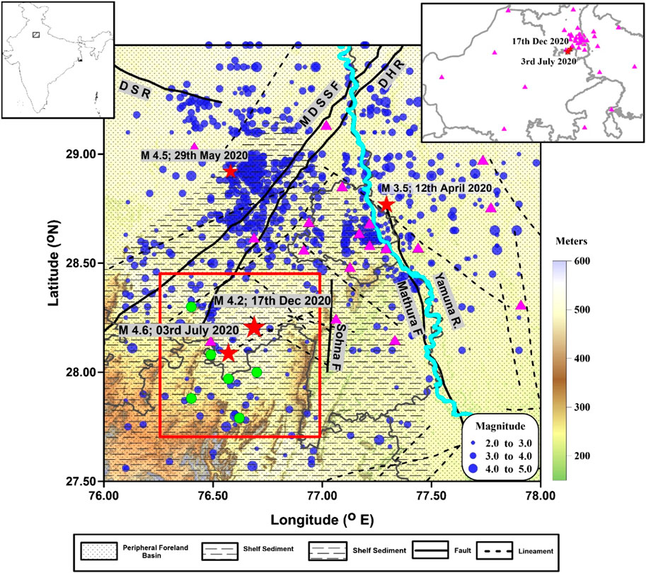
FIGURE 1. Seismotectonic map of the Delhi NCR overlaid on the topography map of the region. The red rectangle shows the study area considered in the present study. Red stars indicate significant earthquakes in the region during 2020, including the events M4.6 (3rd July 2020) and M4.2 (17th December 2020) that occurred in the study area. The blue circles are the earthquakes (2.0<M<5.0) in the region located during 1960–2022. The magenta triangles are the locations of broadband seismic stations in the region. The seismic stations shown in the inset are used in the analysis for determination of source parameters and waveform inversion. The green circles are events that are used in the stress inversion analysis. The curved lines indicate the state boundary of Delhi, Haryana, and Rajasthan. Thick black lines show the prominent faults and structural elements running across the Delhi NCR, namely, Mahendragarh–Dehradun subsurface fault (MDSSF), Delhi–Haridwar ridge (DHR) to the northwest of NCR Delhi, NS-trending Sohna and Mathura faults, and Delhi–Sargodha ridge (DSR). The mapped lineaments in the region are indicated by dashed lines.

The epicentral regions of both the events are characterized by low as well as sparse seismicity (nearly quiescent-like situation) in an area of ∼100 sq km. Furthermore, analysis of the InSAR (Sentinel-1B) data also showed no significant ground surface deformation resulting from the 2020 events. Conspicuously, identification of the causative source for these events in the field remained challenging. The adjacent regions to the north of it, close to Delhi and Haryana, had witnessed considerable seismic activity. Several moderate-magnitude earthquakes have occurred in the recent past (Figure 1), and the area is also characterized to be seismically very susceptible and vulnerable to great earthquakes (Valdiya, 1976; Chandra, 1992). Many studies have been carried out in the region to characterize seismic sources and regional tectonics (Chouhan, 1975; Verma and Greiling, 1995; Singh et al., 2002; Shukla et al., 2007; Bansal et al., 2009; Pandey et al., 2020). Furthermore, it is undeniable that the Himalayan Thrust system and reactivation of the fault systems of Delhi Fold Belt are the prime causative sources of the seismic hazard in Delhi and adjoining regions (Chandra, 1992; Bilham et al., 2001; Gupta et al., 2013; Shukla et al., 2016). Based on the examination of seismic data (1960–2022), it has been observed that there are sporadic instances of seismic activity dispersed throughout significant faults like Mathura fault, Sohna fault, and various mapped lineaments in the region (Figure 1). The dispersed distribution of seismic activity around these geological structures necessitated additional exploration of the fundamental geological and tectonic mechanisms responsible for such activity. The continuous monitoring and meticulous analysis of seismic events occurring in close proximity to these faults and lineaments contribute significantly toward a comprehensive assessment of the seismic hazards in the region. The ongoing investigation and diligent observation of seismic activity are imperative in order to gain a deeper comprehension of the intricate nature of these geological formations and bolster our capacity to evaluate and alleviate seismic hazards in the region.

In the present study, we analyze the best-recorded broadband data from 26 seismic stations of the national network corresponding to the recent earthquakes on 03 July 2020 and 17 December 2020 for source study and to understand the present-day stress fields responsible for the occurrence of these events in the relatively quiescent region. We also analyze the data for understanding the possible connection between the July 2020 and December 2020 earthquakes by computing the static Coulomb stress. This is carried out by using a uniform slip model as well as the source parameters acquired from the waveform inversion analysis. We also examined the stress consequences of the July 2020 event and its relationship with the December 2020 earthquake. The waveform data recorded at seismic stations located up to ∼500 km from the epicentral zone are used in the source parameter estimation and full-waveform inversion analysis for the fault plane solutions. Furthermore, a stress inversion modeling is carried out for understanding the seismogenesis of the 2020 events, and, subsequently, the causative fault of the events is ascertained based on the orientation of the extensional principal stress field.

Geology and seismotectonics

The study area is located in the northernmost part of the Aravalli Range, bordering the regions of Haryana and northeastern parts of Rajasthan. The area is overlaid with sedimentary deposits on both sides, forming alluvium plains to the east and west of the Aravalli. The folded Aravalli range is the main tectonomorphic feature in eastern Rajasthan. The ensemble consists of Proterozoic age Aravalli and Delhi Supergroup rocks, which are on top of the Archean basement. Most of the Aravalli range consists of Delhi Supergroup rocks (Verma and Greiling, 1995; Bansal et al., 2021). In Delhi, both intrusive and extrusive rocks are found in a large area.

The Aravalli–Delhi orogenic belt abundantly occupies faults, fractures, and lineaments oriented criss-cross along NE–SW, NNE–SSW to NE–SW, and NW–SE to WNW–ESE directions (Singh, 1988). The interrelationship of sedimentary facies and paleo-environments of the Delhi Supergroup can best be explained by an evolving intra-cratonic rift-basin model that is found to be comparable to several well-studied continental rift basins. Ravindra and Bakliwal (1983) discussed some of the faults in their studies and found them related to the Delhi orogeny. However, a few of them were characterized by some unique sedimentary and volcanic features, which indicate syn-sedimentary origins (Singh, 1982), and they are found to be seismically active. A prominent fault/ridge system to the NW of the study region, called the Delhi–Haridwar ridge (DHR) and Mahendragarh–Dehradun subsurface fault (MDSSF), is oriented NE–SW, and prominent small-to-moderate earthquakes have been reported along it (Figure 1).

The earthquakes originating from nearby sources are typically intraplate, with shallow focal depth and intermediate magnitudes. The seismic activity is observed to be clustered in three distinct regions: (a) to the west of Delhi, (b) in close proximity to Sonipat, and (c) surrounding Rohtak (Prakash and Shrivastava, 2012). Over time, it has been noted that the majority of earthquakes in the western portion of Delhi are linked to the Sohna fault, which trends in a north–south direction. These earthquakes also occur along the tri-junction of the Delhi–Haridwar ridge and the Delhi–Sargodha fault as well as along the axis of the DFB (Das et al., 2018). In addition, there are other earthquake occurrences scattered around this region. No mapped faults or features are specifically related with activities around Rohtak and Sonipat. The activity in this area is likely caused by the extension and intersection of multiple unmapped faults that are buried behind a thick layer of alluvium and the Delhi–Hardwar ridge. Delhi is experiencing a significant number of scattered earthquakes, which may be attributed to the presence of unexplored active faults. In recent years, a fault near Khanpur in South Delhi was detected (Bansal et al., 2021).

Data analysis and methodology

Earthquake activity in Delhi and its surrounding regions was monitored using 17 permanent broadband seismic stations that are maintained by the National Center for Seismology (NCS) under the aegis of the Ministry of Earth Sciences, India. Later, eight additional seismic stations were deployed in the region soon after the recent earthquake sequence of 2020 (Figure 1). Conspicuously, the present setup of the seismological observatories has improved the detection capability of the NCS, and smaller magnitude earthquakes (i.e., M > 2.0) are being precisely located in and around the Delhi region in near real-time. The earthquakes in the region are being recorded at these seismic stations by using REFTEK 151A-120 tri-axial orthogonal sensors with a flat velocity response in the frequency range 50 Hz–120 s. The VSAT linked network accurately records GPS-synchronized seismological data with a sampling frequency of 100 Hz. In the present study, we analyzed the waveform data of the recent events of 2020 (M_w 4.6 and 4.2) that were recorded by these local seismic stations.

Earthquake data analysis

Well-recorded waveform data at about 14 seismic stations were analyzed using SEISAN software (Havskov and Ottemöller, 2003) to relocate the two recent earthquakes, viz., Mw 4.6 and 4.2 (Figure 1). The P-wave velocity model of the Himalayan foreland basin (Mitra et al., 2011) is considered in this analysis. The arrival times of P- and S-waves were picked on the vertical and horizontal seismograms, respectively, in the case of both the events. The average root mean square (rms) errors, which indicate a measure of the time difference between the observed and estimated travel times, were found to be ∼0.40. Upon analysis, it was determined that the uncertainty associated with identifying the epicenters and determining the focal depth of both events fell within the acceptable range, as the error margin was found to be within the permissible limits of ±2.0 km and ±2.4 km, respectively. (Table 1).

TABLE 1

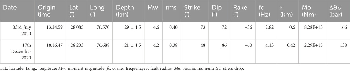
TABLE 1. Hypocenter, focal mechanism, and source parameters of the events.

Furthermore, to characterize the epicentral region, we analyzed earthquake data (NCS catalog) for the period 2000–2022 for a rectangular area (∼100 sq km) covering the study region (Figure 2A). Prior to the analysis, the catalog was de-clustered for duplicate events, foreshocks, and aftershocks, and further it was homogenized by converting different magnitude scales into M_w. A total of 62 events were homogenized in the magnitude range M_w 3.0–4.6. The homogenized data are used in the analysis for estimation of various statistical parameters, viz., cumulative moment release, changes in the magnitude–frequency distribution of earthquakes (b-value), and temporal (year wise) variation of events versus magnitudes (Figures 2B–D), that characterize the sources in any specific region. Figures 2A, D clearly show that most of the activity is concentrated northwest of the epicentral region and during 2004–2012. Throughout the sequence in years 2000–2022, the distribution of magnitudes is similar, except for the 2020 event, which is largest magnitude event recorded in the area.

FIGURE 2

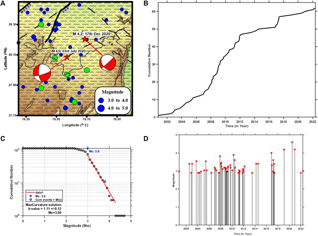
FIGURE 2. (A) Seismicity map of the study area (within 100 sq km from the epicenter of 2020 events) for the period 1960–2022, overlaid on the topography map of the region. The focal mechanisms of the 2020 events (red star) are represented with beach balls. The green circles are the events with magnitude M > 3.0 that are together with the 2020 events (M4.6 and M4.2) used in the stress inversion analysis. The major faults and mapped lineaments are shown as continuous and dashed lines, respectively (source: BHUKOSH Portal, GSI). (B) Plot showing cumulative moment release in Nm versus time in year. (C) Magnitude–frequency distribution plot of earthquakes indicating b-value and Mc of the study area. (D) Annual magnitude variability plot (2000–2022) for the study area.

Waveform inversion

The ISOLA software (Sokos and Zahradnik, 2008) is used in the present study to estimate the fault plane solutions of the events that occurred on 3rd July and 17th December 2020, after constraining the hypocentral location in the previous sub-section. The ISOLA code is developed to invert local and regional full-wave seismograms for single- and multiple-point source models following the iterative deconvolution approach (Kikuchi and Kanamori, 1991). The decomposition in ISOLA as part of the inversion process, namely, volumetric (ISO), compensated linear vector dipole (CLVD), and double couple (DC) stipulates as ISO% + CLVD% + DC% = 100% (Vavryčuk, 2001; Benetatos et al., 2012; Kühn and Vavryčuk, 2013). We considered the waveform data of 14 broadband seismic stations (Figure 1, inset), which are spread across the region with good azimuthal coverage, in the analysis to retrieve the source mechanism, focal depth, and origin time of the events. However, the optimum solution is inferred from the variance reduction function between the observed and synthetic seismograms considering nine seismic stations only, which were matching well. Prior to the analysis, the signal-to-noise ratios at each station were analyzed to fix an appropriate frequency band in which the signal could be inverted. In addition, the instrument effects were removed from the waveforms to obtain the actual ground velocity.

The waveform data were band-pass-filtered in the frequency range (0.2–0.35 Hz) to satisfy the assumption of a point-source model. Green’s functions were computed subsequently along the source-to-receiver paths, over a range of focal depths, using a generic velocity model that is adequate to model a seismogram. In the present study, we considered two different velocity models for the region, viz., Mitra et al. (2011) and Rajat et al. (2023 communicated). After a thorough analysis, it was found that the computed output derived from the Rajat et al. (2023) model exhibited the highest degree of conformity with the observation as compared to other models that were evaluated. Figures 3A, B show a correlation plot between the observed and synthetic waveforms as well as the focal mechanism for a series of focal depths ranging from 2 to 50 km with 2-km intervals for the 03 July 2020 event and from 10 to 50 km with 2-km intervals for the 17 December 2020 event, respectively. In order to avoid the potential trade-offs between the origin time and focal depth, a grid search technique was adopted, and a series of moment–tensor inversions were performed for obtaining an optimum solution over a range of focal depths and origin times to maximize the variance reduction, i.e., correlation. The origin times in the range between −3 s and +3 s were considered in the analyses with a time shift of 1 s from the origin time. Figures 4A, B show the variance reductions that quantify the fitness error between the observed and synthetic seismograms of the events that were computed for the optimum deviatoric and full moment–tensor solutions. The best-fit solutions of the events are eventually achieved for the origin times 13:24:59.0 UTC and 18:16:46.00 UTC of the events on 3rd July 2020 and 17th December 2020, respectively (Table 1). Evidently, the seismic moments of the events M_w 4.6 and 4.2 were obtained to be 8.287E+15 Nm and 2.29E+15 Nm, respectively. The moment magnitude of the events was eventually computed using an empirical relationship dependent on the seismic moment, as proposed by Hanks and Kanamori (1979). The moment–tensor solutions have been obtained at different values of decompositions, say, 0.0% VOL, 31.3% CLVD, and 68.7% DC components.

FIGURE 3

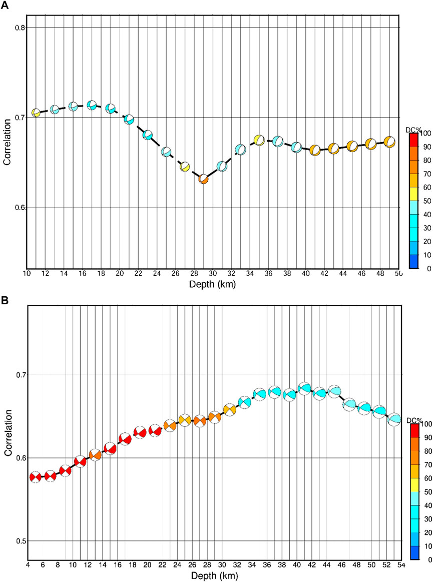
FIGURE 3. (A) Correlation between the observed and synthetic waveforms and focal mechanism as a function of the trial source depth below the epicenter of the 03^rd July 2020 event. Color indicates DC% signifying the correlation. (B) Correlation between the observed and synthetic waveforms and focal mechanisms as a function of the trial source depth below the epicenter of the 17th December 2020 event. Color indicates DC% signifying the correlation.

FIGURE 4

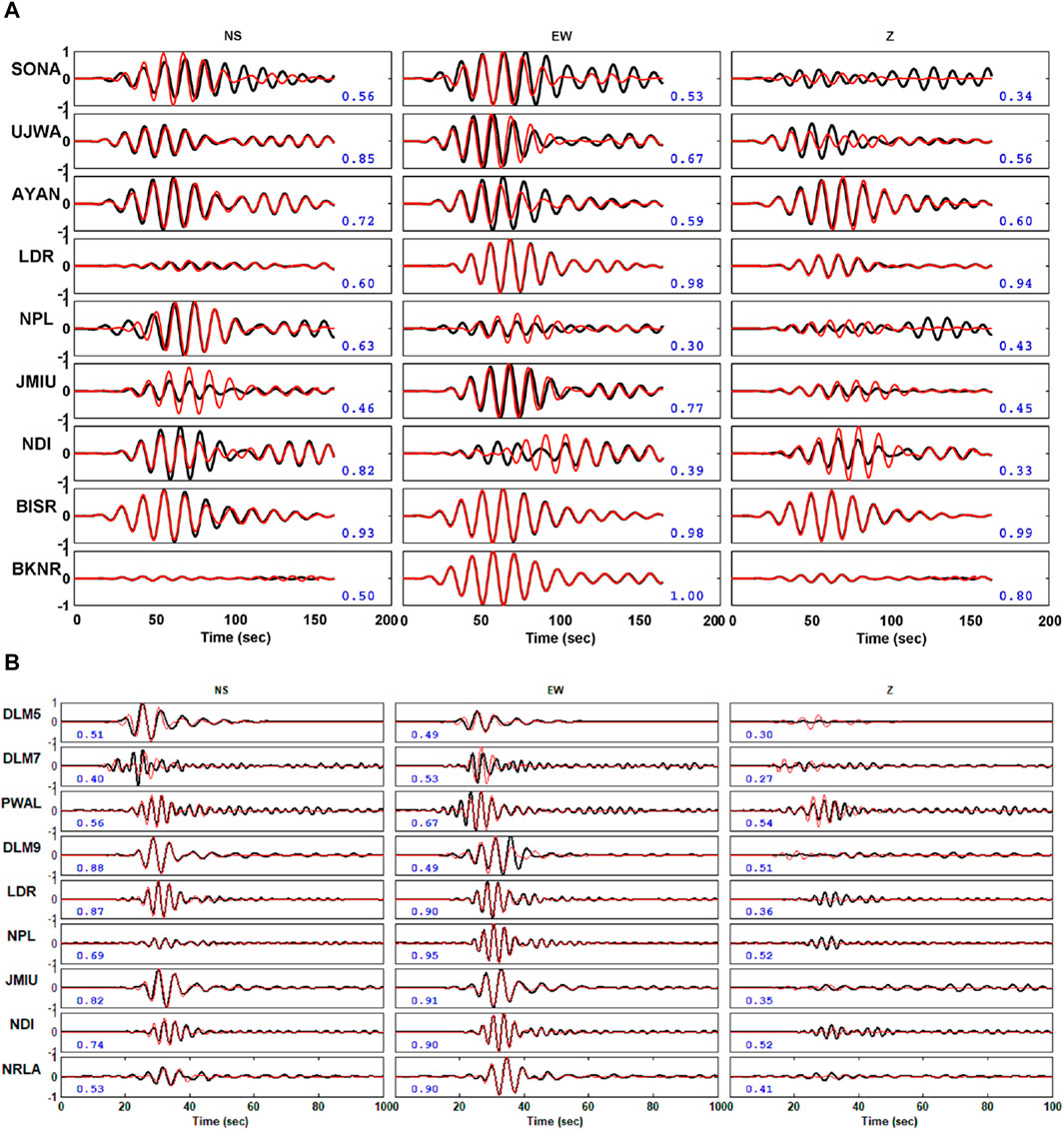
FIGURE 4. (A) Comparison of the observed and synthetic waveforms obtained using the waveform moment tensor inversion approach corresponding to the 03^rd July 2020 event. The black and red waveforms represent the observed and synthetic waveforms, respectively. Blue numbers represent the variance reduction (i.e., correlation) between the observed and synthetic waveforms. (B) Comparison of the observed and synthetic waveforms obtained using waveform moment tensor inversion approach corresponding to the 17th December 2020 event. The black and red waveforms represent the observed and synthetic waveforms, respectively. Blue numbers represent the variance reduction between the observed and synthetic waveforms.

The focal mechanism solutions show normal faulting mechanisms with a minor component of strike–slip with two nodal planes orienting almost NE–SW and NW–SE (Figure 1). The fault parameters of the events that were retrieved from double-couple focal mechanism solutions are listed in Table 1. The uncertainty in the fault plane solution was also performed considering all possible solutions that were matching with the polarities obtained using the stress inversion.

Stress pattern from the inversion of the focal mechanism solution

Stress tensor inversion was carried out to calculate the stress tensors that usually best explain the seismological observations. In the present study, a technique developed by Vavryčuk (2011) and Vavryčuk (2014) is used to determine the orientation of local stress axes along the activated fault/lineament as well as to estimate the stress ratio ‘R’ (also called shape ratio) in the dislocation zone. R is defined as the ratio of the intermediate stresses relative to the maximum horizontal stress and minimum horizontal stress as

$\mathrm{R}=\frac{{\sigma }_2-{\sigma }_3}{{\sigma }_1-{\sigma }_3}.$

In other words, the R value defines the shape of the stress ellipsoid. This technique, which is widely accepted as a powerful tool, is well-known for understanding the stress and tectonic regime of a region. The inputs used in this approach are primarily orientation and slip of the fault nodal planes. In the present study, these input parameters were determined using the fault plane solutions obtained from the moment–tensor inversion of the well-recorded recent events of 2020 (Table 1) as well as P-wave first motion analysis of local events (M > 3.5) that occurred during 2010–2020 (Table 2).

TABLE 2

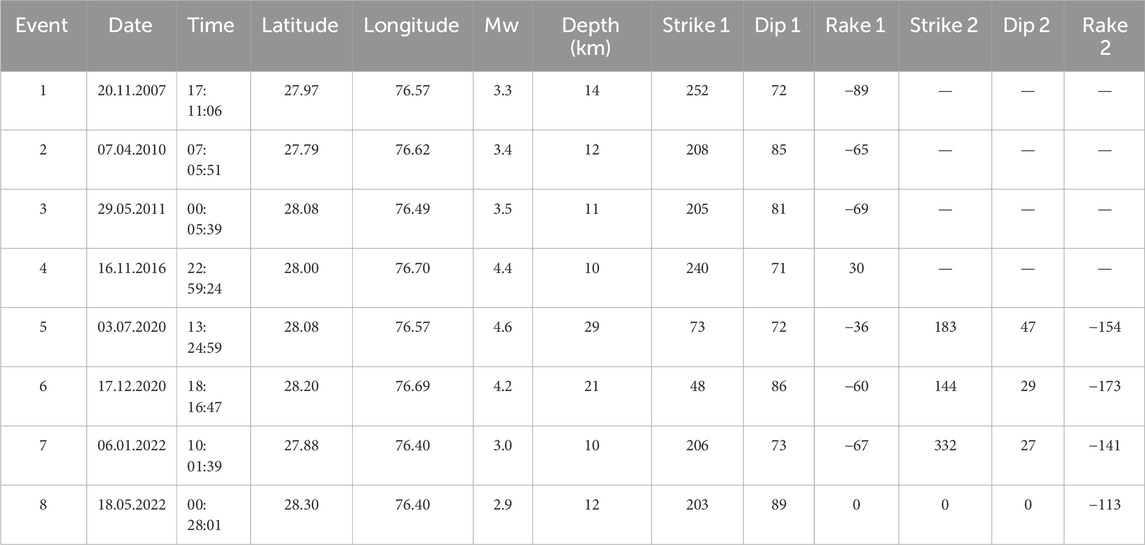
TABLE 2. Focal mechanism solution used for stress inversion.

Any variation in the estimation of the focal mechanism solutions may result in errors in the estimation of the stress ratio and identification of the causative fault plane out of the two nodal planes (Vavrycuk, 2011). However, such limitation could be resolved by incorporating an algorithm useful to identify the causative fault plane and is based on evaluation of the fault instability (I) following the formulation proposed by Vavryčuk (2011; 2014) as

$\mathrm{I}=\mathrm{\tau }-\mathrm{\mu }\left(\mathrm{\sigma }-1\right)/\mathrm{\mu }+\sqrt{1}+{\mathrm{\mu }}^2,$

where μ is the friction coefficient and τ and σ are the normalized shear and normal tractions on a fault, respectively. The method consists of maximizing the slip shear stress component using an iterative algorithm based on robust grid-search inversion over the frictional coefficients ranging from 0.2 to 1.0. The stress axes and fault orientation were determined using the fault instability formulation after a few iterations. In the first iteration, the stresses were obtained by introducing a random perturbation in the focal mechanism. The obtained stress axes later identified the activated causative fault plane, which subsequently was used in the stress inversion analysis. The process was repeated for maximum 100 iterations to obtain the final stress axes. An open-access STRESSINVERSE code written in MATLAB (Vavryčuk, 2014) is used for the stress inversion. In the analysis, four parameters of the stress tensor were recovered that include orientation of three principal stress axes, viz., maximum compressive stress (σ1), intermediate stress (σ2), and minimum compressive stress (σ3), and the shape ratio (R). Furthermore, uncertainties were also ascertained for random perturbation of the focal mechanism by contaminating the signal with an artificial noise. A random noise of 100 realizations was used in the inversion introducing a level of noise of the order 10° in the estimated accuracy of input focal mechanisms. The focal mechanism solutions of total eight events including recent two events of 2020 were inverted to recover the tectonic stress regime in the seismogenic zone (Table 2). Figures 5A–D show the results of the stress inversion analysis indicating an extensional stress field orienting NW–SE with a shape ratio of 0.70 (Table 3).

TABLE 3

TABLE 3. Parameters of the stress tensor from the inversions of the focal mechanisms for the total eight events that occurred in the study region.

FIGURE 5

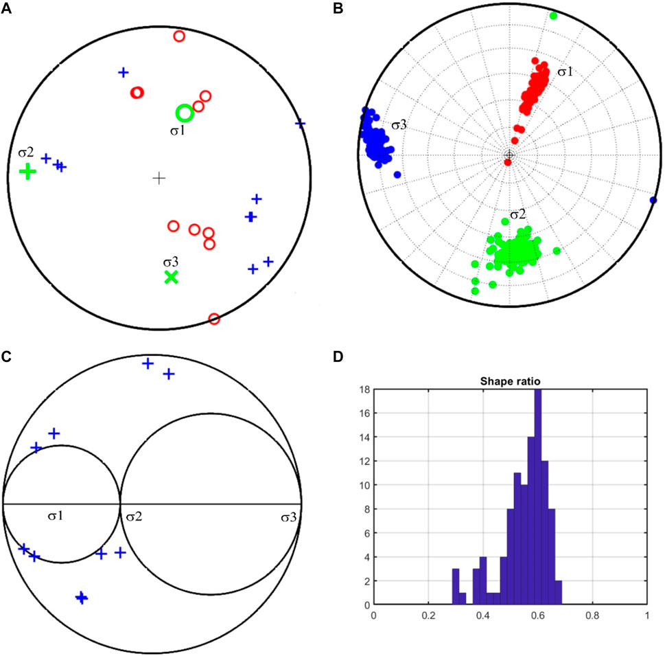
FIGURE 5. Iterative inversion of stress and fault orientations. The plot shows (A) P-axes (red circles) and T-axes (blue plus signs) and the corresponding principal stress directions (σ1, σ2, and σ3). (B) Confidence of principal stress axes retrieved from random perturbation of the focal mechanism dataset given in Table 3. (C) Mohr’s circle diagram with the positions of fault planes. (D) The shape ratio (R) for the 2020 earthquakes that are shown in Figure 2.

Estimation of the source parameter

Stress drop is a measure of the difference between the stress before and after an earthquake, which may potentially be used to distinguish the geodynamic processes causing earthquakes. The strength of an earthquake in the source is represented by seismic moment (Mo). In the present study, we estimated the seismic moment, source radius, and stress drop of the events (Tables 4a, 4b) using amplitude spectra of S-waves following Brune’s model (Brune, 1970), which basically belongs to the circular shear dislocation model. The seismic moment is obtained using the formulation

$M_0=\frac{4\pi {\beta }^3{A}_0}{R\theta \varphi },$

where A₀ is the low-frequency spectral amplitude of S-waves, R is the hypocentral distance, R_θϕ is the radiation pattern of S-waves, β is the S-wave velocity at the source, and ρ is the density at the source. We mention that the correction for free surface amplification and other effects were appropriately accommodated in the radiation factor of S-waves. The corner frequency fc, at which the low frequency and high-frequency asymptotes of amplitude spectra intersect, is used to calculate the radius of a circular fault r using the formulation

$r=\frac{2.34\beta }{2\pi f_C}.$

TABLE 4A

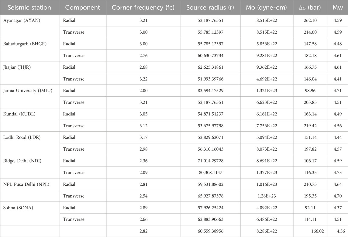
TABLE 4a. Source parameter of the 3rd July 2020 event.

TABLE 4B

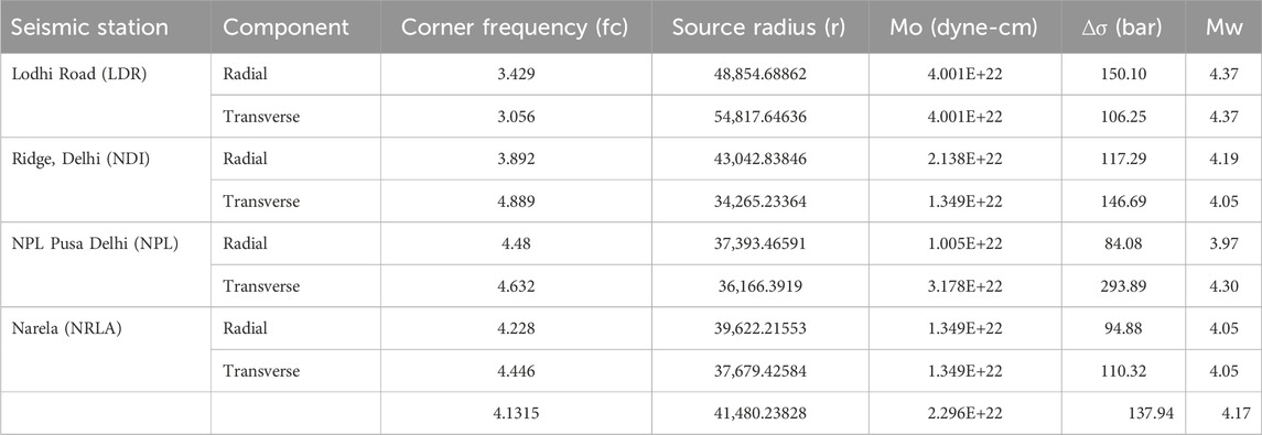
TABLE 4b. Source parameter of the 17th December 2020 event.

Subsequently, the rupture area could be obtained using πr². Furthermore, the stress drops of the events were estimated using the formulation

$\Delta \sigma =\frac{7}{16}\frac{M_0}{r^3}.$

The moment magnitudes of the events were eventually computed using the Hanks and Kanamori (1979) formulation

${\mathrm{M}}_{\mathrm{w}}=2/3*{\log }_{10}{\mathrm{M}}_{\mathrm{o}}-10.73.$

The S-wave spectra at few seismic stations corresponding to the 03 July 2020 and 17 December 2020 events are demonstrated in Figures 6. The average seismic moment, moment magnitude, corner frequency, and stress drop of both the earthquakes are listed in Tables 4a, 4b. As the events were deep-seated (Table 1), the seismic parameters were estimated considering the S-wave velocity of the granitic layer, i.e., 4.53 km/sec. The moment magnitude is obtained to be Mw 4.6 for the 03 July 2020 event and Mw 4.2 for the 17 December 2020 event. The corresponding average seismic moments were found to be 8.28E+15 Nm and 2.29E+15 Nm, and the respective stress drops were estimated to be ∼164 and 137 bars. Such higher stress drops for the intraplate events corroborate well with the results obtained earlier for small-to-moderate magnitude earthquakes (Allmann and Shearer, 2009; Kumar et al., 2014; Sairam et al., 2018). In a recent study, ∼26 bar stress drop was estimated for a relatively small magnitude earthquake (M_w 3.5) that had occurred close to the northeastern part of the National Capital Territory of Delhi. Shearer et al., (2006) and Pandey et al., (2020) emphasized even higher stress drops for the events of intraplate origin with focal mechanism showing relatively a high fraction of normal faulting.

FIGURE 6

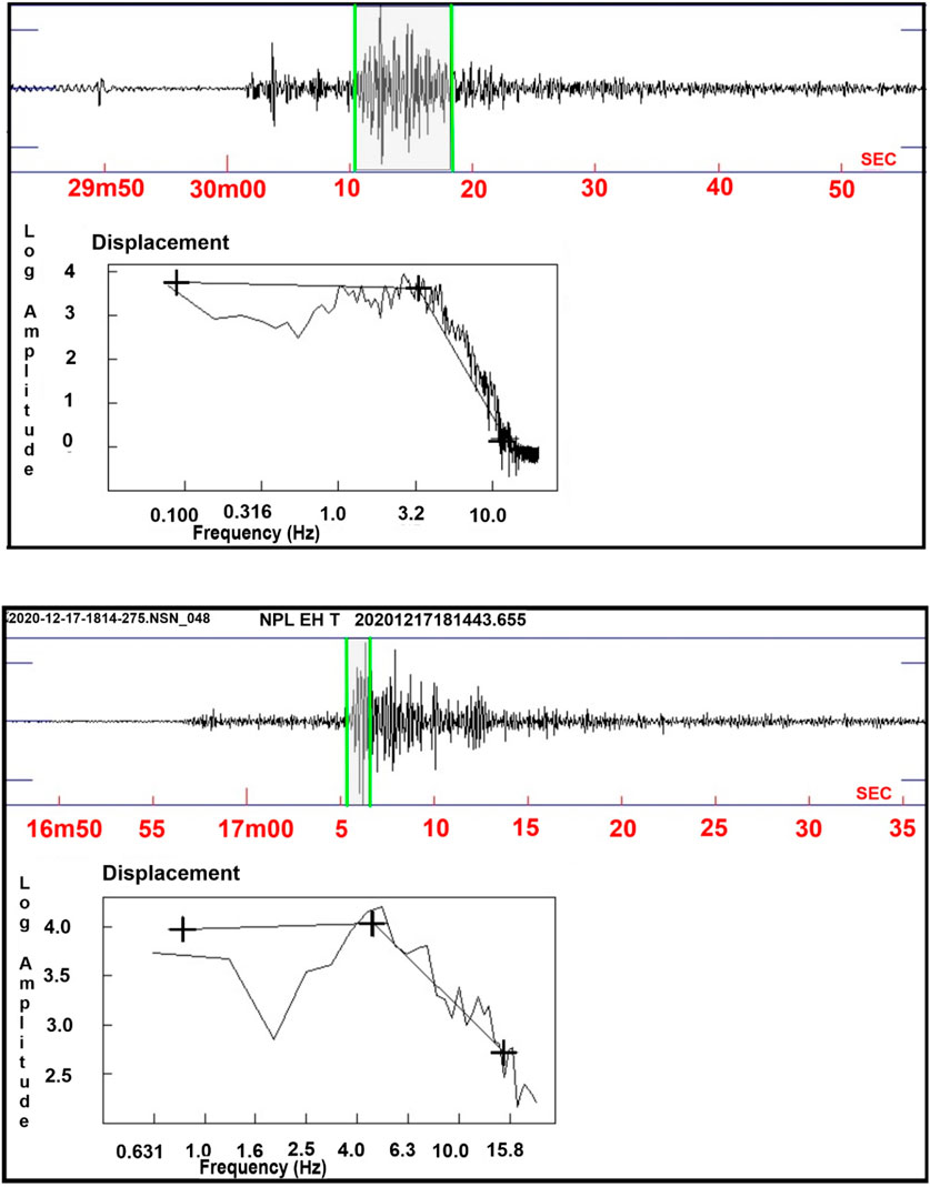
FIGURE 6. upper panel shows the waveforms and its amplitude spectrum for the 03^rd July 2020 (M 4.6) event using data recorded at the AYAN broadband seismic station. The lower panel shows the waveforms and its amplitude spectrum for the 17th December 2020 (M 4.2) event using data recorded at the NPL broadband seismic station. The estimated amplitude spectral parameters, viz., amplitude and corner frequency, from the waveform analysis are given in Tables 4a, 4b.

Coulomb stress change analysis

The seismic fault rupture results in accumulation of the forces that cause a lasting alteration in the stress field in a region nearby the earthquake location, and it is termed as static stress change. Such a change is found to be influenced by different parameters, namely, earthquake location, rupture shape, and type of fault motion (Mitsakaki et al., 2006). One way to quantify this change is through the Coulomb failure function (ΔCFF) analysis, which is influenced by variations in both shear stress (Δτs) and normal stress (Δσn). The change in failure stress, ΔCFF, can be determined using the following equation:

$\Delta \sigma \mathrm{f}=\Delta {\mathrm{\tau }}_{\mathrm{s}}+\mathrm{\mu }’\Delta {\mathrm{\sigma }}_{\mathrm{n}},$

where µ' is effective coefficient of friction on the fault that ranges between 0.2 and 0.8, depending on the fault mechanism, and it accounts for the unknown impact of changes in pore pressure (King et al., 1994; Mouyen et al., 2010). The parameters Δσ_n, Δσf, and Δτ_s are normal stress, shear stress, and shear strength, respectively.

Coseismic static Coulomb stress changes caused due to an event play a crucial role in earthquake-triggering and clustering processes and have a significant impact on the occurrence of aftershocks and subsequent mainshocks in the region (Deng and Sykes, 1997; Harris, 1998; Stein, 1999; Freed and Lin, 2001; King et al., 2001; Freed, 2005; Steacy et al., 2005; Parsons et al., 2008). A small and rapid increase in static stress of less than 0.01 MPa can shorten the time taken for an earthquake to happen; however, a similar drop in static stress can postpone the occurrence of an earthquake (Marsan, 2006; Parsons et al., 2008; Toda et al., 2012; Kariche et al., 2018). When the shear stress loading on the fault surpasses the shear strength, resulting in an accelerated rupture, a positive Δσf is observed. In this particular scenario, the initial seismic event has the potential to expedite the deterioration of a neighboring fault in close proximity. If the change in the normal stress exhibits a negative value, it implies that the shear strength is enhanced and the loading is reduced. Consequently, it can delay the second event from the impending failure and leads it into a region commonly referred to as “stress shadow.” However, a positive change in the Coulomb failure stress transfer within the specific area surrounding the mainshock leads the existing sources into a state of extreme proximity to failure.

The Coulomb stress change analysis computes stress variations transpiring on a designated recipient fault based on the fault slip model (King et al., 1994; Lin and Stein, 2004; Ma et al., 2005; Toda, 2008; Toda, 2008; Ishibe et al., 2011). In addition, various researchers have assimilated the fault plane solutions in computing the Coulomb stress variation (Hardebeck et al., 1998; Meier et al., 2014; Asayesh et al., 2020). Furthermore, using the Coulomb stress analysis, several researchers have inferred that the fault planes may undergo induced stress along the nodal planes ( Wu et al., 2017; Asayesh et al., 2020). The present study is focused on two consequent significant earthquakes (M4.6 of July 2020 and M4.2 of December 2020) that had occurred in the northern part of the Alwar district and to the southwest of the Delhi NCR, within a very short span of time of about 5 months. Considering the proximity of both events, a potential connection between the fault ruptures, stress transfer, and fault interaction is expected. Consequently, the Coulomb failure analysis was carried out to understand whether the first event (M4.6, July 2020) has potentially led to the advancement of the triggering process for the second event (M4.2, December 2020). In order to analyze the potential correlation between both the seismic events, we used Coulomb 3.3 software, which uses elastic half-space modeling techniques.

In the analysis, we assumed an elastic half-space, an apparent coefficient of friction of 0.4, a shear modulus of 32 GPa, and a Poisson’s ratio of 0.25, which allowed us to compute the static Coulomb stress variations as described by Toda et al. (2011a); Toda et al. (2011b). The present investigation involves computation of the static stress alteration on stationary receiver earthquake ruptures and optimally aligned faults. This is accomplished by employing the effective coefficient of friction (µ') of the fault, in conjunction with the strike, dip, and rake information of the fault as well as its hypocentral parameters. The specific receiver fault approach was used to assess the impact of static stress variations induced by the earthquake that occurred in July 2020 on the fault responsible for the earthquake that occurred in December 2020. The inferred model (Figure 3) indicated that the fault is oriented in a NE–SW direction, exhibiting characteristics of a normal fault with a minor strike–slip component (Table 2). This plane was further used as a source plane for the Coulomb stress changes caused by the July 2020 earthquake. Figure 7 demonstrates the Coulomb stress variations resulting from the July 2020 event that is considered a source fault, which refers to the fault plane that experienced slip during the earthquake. However, the source of the event of December 2020 is considered a receiver fault in the analysis. Evidently, four stress lobes were obtained that exhibited positive values, and three stress lobes demonstrated negative values. The initial classification, however, showed a pair of lobes exhibiting pulses orienting southwest and southeast, in addition to another pair of lobes displaying pulses orienting north–northeast and east–southeast. It is to be mentioned that the selection of the specific nodal plane is based on the mapped fault by GSI (source: BHUKOSH web portal). The analysis indicated a positive Coulomb stress change in proximity to the northeast segment of the fault (Figure 7A), due to the July 2020 event which characterized this segment as a potential zone for future failure.

FIGURE 7

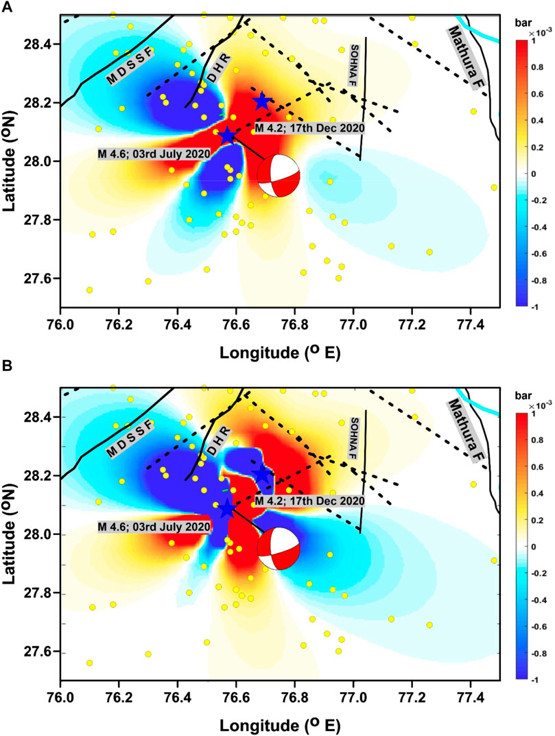
FIGURE 7. Plot showing the Coulomb stress change in the region considering the fault plane solutions of both events (M4.6, July 2020 and M4.2 December 2020 events). (A) The Coulomb stress computed at a depth of 25 km considering the fault plane of the 03rd July 2020 event as a source fault and nodal plane 1 having strike 48, dip 86, and rake −60 of the 17th December 2020 event (Table 2) as a receiver fault, (B) The Coulomb stress computed at a depth of 25 km considering the fault plane of the 03rd July 2020 event as a source fault and nodal plane 2 of the 17th December 2020 event having strike 144, dip 29, and rake −173 (Table 2). The yellow circle denotes past seismic activity occurred during 1960–2022. Thick black lines and dashed lines represent major faults and lineaments, respectively. The blue stars are the epicenter of the 2020 events.

Result and discussion

In the present study, we investigated recent two significant earthquakes that occurred in the Delhi NCR during 2020 to characterize the sources and seismogenesis of the study region. The events were relocated precisely with rms error ∼0.40, considering a P-wave velocity model of the Himalayan foreland basin (Mitra et al., 2011). The events were found to be in proximity, with a separation of ∼10 km, and they are located close to a NE–SW-trending lineament mapped in the study region (Figure 2). Full-waveform inversion using ISOLA software indicates deep-seated focal depths of the events in the mid-crustal range, i.e., >20 km (Table 2). The focal mechanisms of the events demonstrate two distinct nodal planes orienting in the NE–SW and NW–SE directions, which appear to be plausible according to the tectonic settings in the study region. Focal mechanisms of both the events, indicating normal faults with slightly dextral strike–slip movement along NE, however, corroborate well with the lineament mapped in the vicinity of the events. Interestingly, the past earthquakes in the adjacent regions close to the Delhi NCR have mostly witnessed normal faulting with minor strike–slip components, orienting in the NNE direction parallel to the mapped major faults such as DHR and MDDSF.

Stress inversion analysis yields stress parameters, viz., focal sphere with compression (P) and tension (T) axes together with best-fit principal stresses, stereogram of the principal stresses with uncertainties, Mohr circle, and the histogram of the shape ratio (Figures 5A–D). The predominant orientation of the P-axes (red circles) suggests a maximum shortening in the NE direction, in the source region, as depicted in the stereogram (Figure 5B). Evidently, the azimuth of the principal stress, σ1 (red dots), is found to be approximately N25°. Interestingly, the azimuth of σ1 correlates well with the P-axis orientation. The dominant tectonic style is usually determined on the basis of resulting plunge values of σ1 (red dots), σ2 (green dots), and σ3 (blue dots), which are obtained to be around 52°, 38°, and 10°, respectively. The σ1 axis is found closest to the vertical position (highest plunge), indicating the dominance of the extensional stress regime in the region.

The principal stress ratio “R” is determined to be 0.7 (Figure 5D; Table 3). Using the R value, the dominant tectonic regime of the study region can be ascertained based on the stress regime index (R′), which purely depends on the plunge of the three principal stress axes (Kassaras and Kapetanidis, 2018). The factor ‘R′’ may be calculated using the shape ratio ‘R’ as well as the direction of the principal axes (Delvaux et al., 1997; Czirok, 2016). Accordingly, in case of (i) R′ = R; σ1 is found to be vertical and the tectonic stress regime would generally be considered extensional, i.e., of the normal slip type, (ii) R′ = 2 - R; σ2 is found to be vertical in such a case, and the tectonic stress regime would generally be of strike–slip nature, and (iii) R′ = 2 + R; σ3 is found to be vertical, and the tectonic stress would generally be of the thrust regime in this case. Conspicuously, the value of R′ would always be ranging between 0 and 3 as R normally varies from 0 to 1, indicating a clear extensional regime to radial compressional regime following a linear progression (Czirok, 2016). In the present study, σ1 is found to be almost vertical, suggesting a situation where the value of R′ equals to that of R, indicating the presence of normal faults in the region. According to the formula proposed by Zoback (1992), the direction of maximum horizontal stresses (Sh_max) can be determined based on the azimuth and the plunge of the principal stress axes. The Sh_max azimuth is calculated to be N15°E (azimuth of T + 90°) for the study region (Table 3), suggesting the region to be subjected to normal faults with strike–slip faulting and Sh_max direction almost to the north. The stress regime for the present study region is obtained using very limited data, suggesting the region to be heterogeneous; however, the result could be improved based on more available fault plane solutions for the nearby regions. Yadav et al. (2022) carried out a study for the Delhi–Aravalli region and suggested that the maximum principal stress in the region is oriented to N–S to NE–SW and is parallel to the Delhi–Aravalli fold belt, which, however, corroborates well with the findings of the present study.

The moment magnitude of both the events, that occurred on 03 July 2020 and 17 December 2020, was found to be Mw 4.6 and 4.2, respectively. Furthermore, the average seismic moments of the respective events were obtained at 8.28E+15 Nm and 2.29E+15 Nm with stress drops 166 and 138 bars, respectively. Such high stress drops for the intraplate earthquakes corroborate well with the earlier findings for the small- to moderate-sized earthquakes (Allmann and Shearer, 2009; Kumar et al., 2014; Sairam et al., 2018). Usually the stress drop, on occurrence of an earthquake, is influenced by several factors including source geometry, faulting style, tectonic deformation rate, stress regime, rock composition, and focal depth (Kaneko and Shearer, 2014; Goebel et al., 2015). The variation in the stress drop is, however, attributed to the source model assumptions (Huang et al., 2016). In a study, ∼26 bar stress drop was estimated for a relatively small magnitude earthquake (M_w 3.5) that had occurred close to the northeastern part of the National Capital Territory of Delhi. Shearer et al. (2006) and Pandey et al. (2020) suggested even higher stress drops for the events of the intraplate origin with the focal mechanism showing relatively a dominant normal faulting.

Coulomb stress modeling with a fixed receiver fault plane (Figure 7), that is a correlation between the loading lobes, indicated a close interaction between the earthquakes. The Coulomb stress variation map computed using the July 2020 event as a source fault and the December 2020 event as a receiver fault showed that the previous event transferred stress which promoted the failure of the later event (Figure 7A). The December 2020 fault rupture is located in a loading zone which is clearly identified by a positive stress change in this portion. The slip on the July 2020 fault probably increased the stress at the receiver fault and triggered the December 2020 earthquake. Evidently, the later event was potentially triggered by a stress change of 0.002–0.004 bars. The observed alteration in the transferred Coulomb stress resulting from the July 2020 event is found to be causative for triggering the failure of the December 2020 event. The link between the two earthquakes is mainly related to the existence of faults with different types of motion in Aravalli belts, including the N15E-trending normal fault.

The Aravalli range that witnessed the two recent significant tremors is largely composed of an Archean–Proterozoic crystalline basement overlain with fold belts that witnessed multiple episodes of metamorphism and deformation during the Precambrian (Roy et al., 1995; Gupta et al., 1997; Sinha-Roy et al., 1998). The major tectonic features in the region show a predominant NE–SW trend that probably controls the regional tectonics (Gupta et al., 1997). Many of these stratigraphic features that are tectonized (Chetty, 2017) signify the mapped NE–SW lineaments in the region. In the vicinity of the source zone, the prime deformation is observed along the NE-trending ridge fault system, i.e., DHR and MDSSF, characterized by a normal fault with the strike–slip component (Prakash and Shrivastava, 2012). The Sohna and Mathura faults in the region, located to the east of the source zone, were also found to be quite active (Chouhan, 1975; Pandey et al., 2020). The activity might have upsurged the transfer of stresses and their accumulation along the minor active faults/lineaments mapped in the region. It corroborates well with the Coulomb stress pattern (Figure 7A). The seismicity analysis performed using the earthquake catalog complete for magnitudes of 3.0 and above revealed that the epicentral region displayed a reduced rate of seismic activity in comparison to the adjacent regions. The b-value is a measure of the frequency–magnitude distribution of earthquakes in a given region, with higher values indicating a higher likelihood of smaller magnitude earthquakes. The b-value of 1.1 ± 0.12 from the present study suggests that the region is less likely to experience significant seismic activity and is rather more prone to the smaller-magnitude earthquakes (Figures 2C, D). It is worth noting that the seismic activity in the study region during 2000–2022 was recorded within the magnitude range <4.0.

The epicentral zone of the recent activity falls largely in the seismic zone IV (seismically a hazardous zone) of the seismic zonation map of India (BIS, 2002). It is indicative of frequent occurrence of low- to moderate-magnitude earthquakes (two or more events per year) in the region, which is quite intriguing as the region is characterized by cratonized terrain with no major tectonic activity in the past. Kumar and Pandit (2020), however, showed earthquake activity to the southwest of the epicentral zone in recent years and suggested the genesis of such small events may possibly cause stress build-up due to northward drifting and collision of the Indian plate. The optimum solution of the stress modeling indicates a dominant normal stress regime in the source region (Figure 5). The confidence level of principle stresses (Figure 5B) further demonstrates the accuracy of the inverted focal mechanisms with a high stress ratio at 0.7 ± 0.05 (Figure 5C). The distribution of fault planes in Mohr’s circle implies a low shear stress (Figure 5D). About 80% of the fault plane solutions located in the lower Mohr’s semi-circle indicate the NE orientation of the source having a low friction coefficient of ∼0.5. It is emphasized that only a few seismic events in the source region with low activity limited our analysis in achieving accurate inversion to estimate the most likely orientation of the source and stress regime.

Several researchers have suggested that a low friction coefficient in a weak zone along the fault may be causative for seismic activity (Pınar et al., 2010; Fojtíková and Vavryčuk, 2018; Abdelfattah et al., 2020). Furthermore, a low friction coefficient indicates low stress drops in the source, as high shear stress may not be accumulated in extensional tectonics (Abdelfattah et al., 2020). A low friction coefficient, as obtained from the present study, hence characterizes the seismicity in the region. However, the friction coefficient is rather an unstable parameter, and therefore an extensive dataset of accurate focal mechanisms would be required to achieve a better result. Geologically, the epicentral area is composed of gneissic granites and alluvium, which indicate a strong foliation formed on account of shearing stress (Roy, 1976; Chetty, 2017). The shearing of platy minerals like, mica schist, biotite, and chlorite in the vicinity region along the foliation direction might have reactivated the faults/lineaments in the region.

Conclusion

The source parameters of the 03rd July 2020 and 17th December 2020 earthquakes that occurred in the vicinity of Delhi have been estimated using well-recorded data by the seismic network of the Delhi region. The focal mechanism solutions of the events were constructed using the waveform inversion approach, which suggested a normal faulting mechanism with a slightly strike–slip component. The optimum solution reflects a contemporary shear stress regime characterized by major compressive stress (σ1) with 52° plunge and trending 27° NE, intermediate compressive stress (σ2) with 38° plunge and trending 187° SW, and minor compressive stress (σ3) with 10° plunge and trending 285° SE, which corresponds to a dominant normal stress regime that was ascertained using the stress field inversion. The stress regime to the northern and eastern parts of the source zone of the M4.6 earthquake was found to be increased by 0.004–0.008 bars, surpassing the threshold value for triggering an earthquake. Such enhancement in the pressure changes due to the July 2020 event probably triggered the earthquake that occurred on December 2020. However, the stress variations in the off-fault region that is in the peripheral areas adjacent to the main fault, namely, along the Sohna fault and MDSSF fault, due to July event of 2020 were found insignificant. We suggest that the events had occurred along the pre-existing NE–SW lineament mapped in the vicinity and the stress drops for both the events were found to be 166 bar and 138 bars, respectively, that fall well within the range accepted for the intraplate earthquakes. Furthermore, these values of stress drops were also found to be in accordance with the low static friction (∼0.5) for the study region. The moderate stress drops clearly indicate a potential relationship between the local causative source and large-scale regional tectonics in the vicinity region, viz., MDSSF and DHR. The NE–SW-trending lineaments mapped in the region, therefore, appear to be the causative source of the 2020 earthquakes. We emphasize that the seismogenesis of small-to-moderate magnitude earthquakes in the study region may be due to the reactivation of hidden old sutures/weak zones (mapped as lineaments on the surface) owing to stress transfer from the active regional tectonics.

Data availability statement

The raw data supporting the conclusion of this article will be made available on request to the Director of the National Centre for Seismology.

Author contributions

SP provided the research idea and drafted the original manuscript. AP and OM contributed with finalizing the outcomes from the data analysis, their interpretation, and framed the final manuscript. SB and SV analyzed the waveform data and calculated the FMS and stress inversion. All authors contributed to the article and approved the submitted version.

Acknowledgments

The authors thank the Secretary, Ministry of Earth Sciences (MoES), New Delhi, for all necessary support to carry out this research. The scientific and technical staff of NCS, New Delhi, are deeply acknowledged for maintaining the seismic stations and data. The seismic waveform data of the NCS used in the present study are highly acknowledged. SB highly acknowledged the DESK, IITM, Pune, for the fellowship under MRFP. The authors also thank Ross Stein and his team for freely available Coulomb software, which is used in the computation of Coulomb stress.

Conflict of interest

The authors declare that the research was conducted in the absence of any commercial or financial relationships that could be construed as a potential conflict of interest.

Publisher’s note

All claims expressed in this article are solely those of the authors and do not necessarily represent those of their affiliated organizations, or those of the publisher, the editors, and the reviewers. Any product that may be evaluated in this article, or claim that may be made by its manufacturer, is not guaranteed or endorsed by the publisher.

References

Abdelfattah, A. K., Al-amri, A., Sami Soliman, M., Zaidi, F. K., Qaysi, S., Fnais, M., et al. (2020). An analysis of a moderate earthquake, eastern flank of the Red Sea, Saudi Arabia. Earth, Planets Sp. 72, 34. doi:10.1186/s40623-020-01159-5

CrossRef Full Text | Google Scholar

Allmann, B. P., and Shearer, P. M. (2009). Global variations of stress drop for moderate to large earthquakes. J. Geophys. Res. Solid Earth 114. doi:10.1029/2008JB005821

CrossRef Full Text | Google Scholar

Asayesh, B. M., Zafarani, H., and Tatar, M. (2020). Coulomb stress changes and secondary stress triggering during the 2003 (Mw 6.6) Bam (Iran) earthquake. Tectonophysics 775, 228304. doi:10.1016/j.tecto.2019.228304

CrossRef Full Text | Google Scholar

Bansal, B. K., Mohan, K., Haq, A. U., Verma, M., Prajapati, S. K., and Bhat, G. M. (2021). Delineation of the causative fault of recent earthquakes (april-may 2020) in Delhi from seismological and morphometric analysis. J. Geol. Soc. India 97, 451–456. doi:10.1007/s12594-021-1711-5

CrossRef Full Text | Google Scholar

Bansal, B. K., Singh, S. K., Dharmaraju, R., Pacheco, J. F., Ordaz, M., Dattatrayam, R. S., et al. (2009). Source study of two small earthquakes of Delhi, India, and estimation of ground motion from future moderate, local events. J. Seismol. 13, 89–105. doi:10.1007/s10950-008-9118-y

CrossRef Full Text | Google Scholar

Benetatos, C., Malek, J., and Verga, F. (2012). Moment tensor inversion for two micro-earthquakes occurring inside the Háje gas storage facilities, Czech Republic. J. Seismol. 17, 557–577. doi:10.1007/s10950-012-9337-0

CrossRef Full Text | Google Scholar

Bilham, R., Gaur, V. K., and Molnar, P. (2001). Himalayan seismic hazard. Sci. (80- 293, 1442–1444. doi:10.1126/science.1062584

PubMed Abstract | CrossRef Full Text | Google Scholar

Brune, J. N. (1970). Tectonic stress and the spectra of seismic shear waves from earthquakes. J. Geophys. Res. 75, 4997–5009. doi:10.1029/jb075i026p04997

CrossRef Full Text | Google Scholar

Chandra, U. (1992). Seismotectonics of himalaya. Curr. Sci. 62, 40–71.

Google Scholar

Chetty, T. R. K. (2017). The Aravalli-Delhi orogenic belt. Proterozoic Orogens India, 267–350. doi:10.1016/B978-0-12-804441-4.00005-5

CrossRef Full Text | Google Scholar

Chouhan, R. K. S. (1975). Seismotectonics_of_Delhi_Region.pdf. Proc. Indian Nat. Sci. Acad. 41 (A), 429–447.

Google Scholar

Czirok, L. (2016). Analysis of stress relations using focal mechanism solutions in the Pannonian basin. Geosciences Eng. 5/8, 65–84.

Google Scholar

Das, R., Mukhopadhyay, S., Kant, R., and Baidya, P. R. (2018). Lapse time and frequency-dependent coda wave attenuation for Delhi and its surrounding regions. Tectonophysics 738–739, 51–63. doi:10.1016/j.tecto.2018.05.007

PubMed Abstract | CrossRef Full Text | Google Scholar

Delvaux, D., Moeys, R., Stapel, G., Petit, C., Levi, K., Miroshnichenko, A., et al. (1997). Paleostress reconstructions and geodynamics of the Baikal region, Central Asia, Part 2. Cenozoic rifting. Cenozoic Rift. Tectonophys. 282, 1–38. doi:10.1016/S0040-1951(97)00210-2

CrossRef Full Text | Google Scholar

Deng, J., and Sykes, L. R. (1997). Evolution of the stress field in southern California and triggering of moderate-size earthquakes: a 200-year perspective. J. Geophys. Res. Solid Earth 102 (B5), 9859–9886. doi:10.1029/96jb03897

CrossRef Full Text | Google Scholar

Fojtíková, L., and Vavryčuk, V. (2018). Tectonic stress regime in the 2003–2004 and 2012–2015 earthquake swarms in the Ubaye Valley, French Alps. Pure Appl. Geophys. 175, 1997–2008. doi:10.1007/s00024-018-1792-2

CrossRef Full Text | Google Scholar

Freed, A. (2005). Earthquake triggering by static, dynamic, and post-seismic stress transfer. Annu. Rev. Earth Planet. Sci. 33, 335–367. doi:10.1146/annurev.earth.33.092203.122505

CrossRef Full Text | Google Scholar

Freed, A. M., and Lin, J. (2001). Delayed triggering of the 1999 Hector Mine earthquake by viscoelastic stress transfer. Nature 411 (6834), 180–183. doi:10.1038/35075548

PubMed Abstract | CrossRef Full Text | Google Scholar

Goebel, T. H. W., Hauksson, E., Shearer, P. M., and Ampuero, J. P. (2015). Stress-drop heterogeneity within tectonically complex regions: a case study of San Gorgonio Pass, southern California. Geophys. J. Int. 202, 514–528. doi:10.1093/gji/ggv160

CrossRef Full Text | Google Scholar

Gupta, S., Mohanty, W. K., Prakash, R., and Shukla, A. K. (2013). Crustal heterogeneity and seismotectonics of the national capital region, Delhi, India. Pure Appl. Geophys. 170, 607–616. doi:10.1007/s00024-012-0572-7

CrossRef Full Text | Google Scholar

Gupta, S. N., Arora, Y., Mathur, R. K., Iqballuddin Prasad, B., and Sahay, T. N. (1997). The Precambrian geology of the Aravalli region, southern Rajasthan and north-eastern Gujarat. Mem. Geol. Surv. India 123, 262.

Google Scholar

Hanks, T. C., and Kanamori, H. (1979). A moment magnitude scale. J. Geophys. Res. Solid Earth 84 (B5), 2348–2350. doi:10.1029/JB084iB05p02348

CrossRef Full Text | Google Scholar

Hardebeck, J. L., Nazareth, J. J., and Hauksson, E. (1998). The static stress change triggering model: constraints from two southern California aftershock sequences. J. Geophys. Res. Solid Earth 103 (B10), 24427–24437. doi:10.1029/98jb00573

CrossRef Full Text | Google Scholar

Harris, R. A. (1998). Introduction to special section: stress triggers, stress shadows, and implications for seismic hazard. J. Geophys. Res. 103, 24347–24358. doi:10.1029/98jb01576

CrossRef Full Text | Google Scholar

Havskov, J., and Ottemöller, L. (2003). SEISAN: the earthquake analysis software. China: Dep. Earth Sci. Univ. Bergen, Norway.

Google Scholar

Huang, Y., Beroza, G. C., and Ellsworth, W. L. (2016). Stress drop estimates of potentially induced earthquakes in the Guy-Greenbrier sequence. J. Geophys. Res. Solid Earth 121, 6597–6607. doi:10.1002/2016JB013067

CrossRef Full Text | Google Scholar

Ishibe, T., Shimazaki, K., Tsuruoka, H., Yamanaka, Y., and Satake, K. (2011). Correlation between Coulomb stress changes imparted by large historical strike-slip earthquakes and current seismicity in Japan. Earth, Planets Space 63 (3), 301–314. doi:10.5047/eps.2011.01.008

CrossRef Full Text | Google Scholar

Kaneko, Y., and Shearer, P. M. (2014). Seismic source spectra and estimated stress drop derived from cohesive-zone models of circular subshear rupture. Geophys. J. Int. 197, 1002–1015. doi:10.1093/gji/ggu030

CrossRef Full Text | Google Scholar

Kariche, J., Meghraoui, M., Timoulali, Y., Cetin, E., and Toussaint, R. (2018). The Al Hoceima earthquake sequence of 1994, 2004 and 2016: stress transfer and poro-elasticity in the Rif and Alboran Sea region. Geophys. J. Int. 212 (1), 42–53. doi:10.1093/gji/ggx385

CrossRef Full Text | Google Scholar

Kassaras, I. G., and Kapetanidis, V. (2018).Resolving the tectonic stress by the inversion of earthquake focal mechanisms. Application in the region of Greece. A tutorial. Germany: Springer International Publishing. doi:10.1007/978-3-319-77359-9_19

CrossRef Full Text | Google Scholar

Kikuchi, M., and Kanamori, H. (1991). Inversion of complex body waves—III. Bull. Seismol. Soc. Am. 81, 2335–2350. doi:10.1785/BSSA0810062335

CrossRef Full Text | Google Scholar

King, G. C., Stein, R. S., and Lin, J. (1994). Static stress changes and the triggering of earthquakes. Bull. Seismol. Soc. Am. 84 (3), 935–953. doi:10.1785/BSSA0840030935

CrossRef Full Text | Google Scholar

King, G. C. P., Cocco, M., Renata, D., and Barry, S. (2001). Fault interaction by elastic stress changes: New clues from earthquake sequences. Adv. Geophys. 44, 1–38. doi:10.1016/S0065-2687(00)80006-0

CrossRef Full Text | Google Scholar

Kühn, D., and Vavryčuk, V. (2013). Determination of full moment tensors of microseismic events in a very heterogeneous mining environment. Tectonophysics 589, 33–43. doi:10.1016/j.tecto.2012.12.035

CrossRef Full Text | Google Scholar

Kumar, H., and Pandit, M. (2020). Recurrent seismicity in Rajasthan State in the tectonically stable NW Indian craton. Iran. J. Earth Sci. 12, 1–9. doi:10.30495/ijes.2020.671653

CrossRef Full Text | Google Scholar

Kumar, S., Kumar, D., and Rastogi, B. (2014). Source parameters and scaling relations for small earthquakes in the Kachchh region of Gujarat, India. Nat. Hazards 73, 1269–1289. doi:10.1007/s11069-014-1133-4

CrossRef Full Text | Google Scholar

Lin, J., and Stein, R. S. (2004). Stress triggering in thrust and subduction earthquakes and stress interaction between the southern San Andreas and nearby thrust and strike-slip faults. J. Geophys. Res. Solid Earth 109. doi:10.1029/2003JB002607

CrossRef Full Text | Google Scholar

Ma, K. F., Chan, C. H., and Stein, R. S. (2005). Response of seismicity to Coulomb stress triggers and shadows of the 1999 M_w = 7.6 Chi-Chi, Taiwan, earthquake. J. Geophys. Res. Solid Earth 110. doi:10.1029/2004JB003389

CrossRef Full Text | Google Scholar

Marsan, D. (2006). Can coseismic stress variability suppress seismicity shadows? Insights from a rate-and-state friction model. J. Geophys. Res. Solid Earth 111 (B6). doi:10.1029/2005jb004060

CrossRef Full Text | Google Scholar

Meier, M. A., Werner, M. J., Woessner, J., and Wiemer, S. (2014). A search for evidence of secondary static stress triggering during the 1992 M_w7.3 Landers, California, earthquake sequence. J. Geophys. Res. Solid Earth 119 (4), 3354–3370. doi:10.1002/2013jb010385

CrossRef Full Text | Google Scholar

Mitra, S., Kainkaryam, S. M., Padhi, A., Rai, S. S., and Bhattacharya, S. N. (2011). The Himalayan foreland basin crust and upper mantle. Phys. Earth Planet. Inter. 184, 34–40. doi:10.1016/j.pepi.2010.10.009

CrossRef Full Text | Google Scholar

Mitsakaki, C., Sakellariou, M., Tsinas, D., and Marinou, A. (2006). Assessment of coulomb stress changes associated with the 1995 aigion earthquake in the gulf of corinth (Greece). Geodetic deformation monitoring: from geophysical to engineering roles. Germany: Springer, 172–180.

Google Scholar

Mouyen, M., Cattin, R., and Masson, F. (2010). Seismic cycle stress change in western Taiwan over the last 270 years. Geophys. Res. Lett. 37. doi:10.1029/2009GL042292

CrossRef Full Text | Google Scholar

Pandey, A. P., Suresh, G., Singh, A. P., Sutar, A. K., and Bansal, B. K. (2020). A widely felt Tremor (ML 3.5) of 12 April 2020 in and around NCT Delhi in the backdrop of prevailing COVID-19 pandemic lockdown: analysis and observations. Geomatics, Nat. Hazards Risk 11, 1638–1652. doi:10.1080/19475705.2020.1810785

CrossRef Full Text | Google Scholar

Parsons, T., Ji, C., and Kirby, E. (2008). Stress changes from the 2008 Wenchuan earthquake and increased hazard in the Sichuan Basin. Nature 454 (7203), 509–510. doi:10.1038/nature07177

PubMed Abstract | CrossRef Full Text | Google Scholar

Pınar, A., Üçer, S. B., Honkura, Y., Sezgin, N., Ito, A., Barış, Ş., et al. (2010). Spatial variation of the stress field along the fault rupture zone of the 1999 Izmit earthquake. Earth, Planets Sp. 62, 237–256. doi:10.5047/eps.2009.12.001

CrossRef Full Text | Google Scholar

Prakash, R., and Shrivastava, J. P. (2012). A review of the seismicity and seismotectonics of Delhi and adjoining areas. J. Geol. Soc. India 79, 603–617. doi:10.1007/s12594-012-0099-7

CrossRef Full Text | Google Scholar

Ravindra, R., and Bakliwal, P. C. (1983). Geological and geomorphological significance of a few mega-lineaments of Northeastern Rajasthan. J. Indian Soc. Photo-Interpretation Remote Sens. 11, 31–37. doi:10.1007/BF02990759

CrossRef Full Text | Google Scholar

Roy, S., Malhotra, G., and Guha, D. (1995). A transect across Rajasthan Precambrian terrain in relation to geology, tectonics and crustal evolution of south central Rajasthan. Mem. - Geol. Soc. India 31, 63–89.

Google Scholar

Roy, S. K. (1976). Tectonic style in the Delhi group of rocks, Western India. Misc. Pub. Geol. Surv. India 31, 239–245.

Google Scholar

Sairam, B., Singh, A. P., and Ravi Kumar, M. (2018). Comparison of earthquake source characteristics in the kachchh rift basin and Saurashtra horst, deccan volcanic province, western India. J. Earth Syst. Sci. 127, 55. doi:10.1007/s12040-018-0957-9

CrossRef Full Text | Google Scholar

Shearer, P. M., Prieto, G. A., and Hauksson, E. (2006). Comprehensive analysis of earthquake source spectra in southern California. J. Geophys. Res. Solid Earth 111. doi:10.1029/2005JB003979

CrossRef Full Text | Google Scholar

Shukla, A., Prakash, R., Singh, R., Mishra, P., and Bhatnagar, A. (2007). Seismotectonic implications of Delhi region through fault plane solutions of some recent earthquakes. Curr. Sci. 93, 1848–1853.

Google Scholar

Shukla, A., Singh, R., Mandal, H. S., Pandey, A., and Shukla, M. (2016). A report on seismic hazard microzonation of NCT Delhi on 1:10,000 scales.

Google Scholar

Singh, S. K., Mohanty, W., Bansal, B. K., and Roonwal, G. (2002). Ground motion in Delhi from future large/great earthquakes in the central seismic gap of the himalayan arc. Bull. Seismol. Soc. Am. - Bull. Seism. Soc. AMER 92, 555–569. doi:10.1785/0120010139

CrossRef Full Text | Google Scholar

Singh, S. P. (1982). Stratigraphy of the Delhi Supergroup in bayana sub-basin northeastern Rajasthan. Rec. Geol. Surv. India 112, 46–62.

Google Scholar

Singh, S. P. (1988). Sedimentation patterns of the Proterozoic Delhi Supergroup, northeastern Rajasthan, India, and their tectonic implications. Sediment. Geol. 58, 79–94. doi:10.1016/0037-0738(88)90007-3

CrossRef Full Text | Google Scholar

Sinha-Roy, S., Malhotra, G., Mohanty, M., and of India, G. S. (1998). Geology of Rajasthan. Geological society of India. Available at: https://books.google.co.in/books?id=dYUhnQAACAAJ.

Google Scholar

Sokos, E. N., and Zahradnik, J. (2008). ISOLA a Fortran code and a Matlab GUI to perform multiple-point source inversion of seismic data. Comput. Geosci. 34, 967–977. doi:10.1016/j.cageo.2007.07.005

CrossRef Full Text | Google Scholar

Steacy, S., Gomberg, J., and Cocco, M. (2005). Introduction to special section: stress transfer, earthquake triggering and time dependent seismic hazard. J. Geophys. Res. Solid Earth 110. doi:10.1029/2005JB003692

CrossRef Full Text | Google Scholar

Stein, R. S. (1999). The role of stress transfer in earthquake occurrence. Nature 402 (6762), 605–609. doi:10.1038/45144

CrossRef Full Text | Google Scholar

Toda, S. (2008). Coulomb stresses imparted by the 25 March 2007 Mw=6.6 Noto-Hanto, Japan, earthquake explain its ‘butterfly’ distribution of aftershocks and suggest a heightened seismic hazard. Earth Planets Space 60, 1041–1046. doi:10.1186/bf03352866

CrossRef Full Text | Google Scholar

Toda, S., Lin, J., and Stein, R. S. (2011a). Using the 2011 M w 9.0 off the Pacific coast of Tohoku Earthquake to test the Coulomb stress triggering hypothesis and to calculate faults brought closer to failure. Earth, Planets Space 63, 725–730. doi:10.5047/eps.2011.05.010

CrossRef Full Text | Google Scholar

Toda, S., Lin, J., and Stein, R. S. (2011b). Using the 2011 Mw 9.0 off the Pacific coast of Tohoku Earthquake to test the Coulomb stress triggering hypothesis and to calculate faults brought closer to failure. Earth, Planets Space 63, 725–730. doi:10.5047/eps.2011.05.010

CrossRef Full Text | Google Scholar

Toda, S., Stein, R. S., Beroza, G. C., and Marsan, D. (2012). Aftershocks halted by static stress shadows. Nat. Geosci. 5 (6), 410–413. doi:10.1038/ngeo1465

CrossRef Full Text | Google Scholar

Valdiya, K. S. (1976). Himalayan transverse faults and folds and their parallelism with subsurface structures of North Indian plains. Tectonophysics 32, 353–386. doi:10.1016/0040-1951(76)90069-X

CrossRef Full Text | Google Scholar

Vavryčuk, V. (2001). Inversion for parameters of tensile earthquakes. J. Geophys. Res. Solid Earth 106, 16339–16355. doi:10.1029/2001JB000372

CrossRef Full Text | Google Scholar

Vavryčuk, V. (2011). Principal earthquakes: theory and observations from the 2008 west bohemia swarm. Earth Planet. Sci. Lett. 305, 290–296. doi:10.1016/j.epsl.2011.03.002

CrossRef Full Text | Google Scholar

Vavryčuk, V. (2014). Iterative joint inversion for stress and fault orientations from focal mechanisms. Geophys. J. Int. 199, 69–77. doi:10.1093/gji/ggu224

CrossRef Full Text | Google Scholar

Verma, P. K., and Greiling, R. O. (1995). Tectonic evolution of the Aravalli orogen (NW India): an inverted Proterozoic rift basin? Geol. Rundsch. 84, 683–696. doi:10.1007/BF00240560

CrossRef Full Text | Google Scholar

Wu, J., Cai, Y., Li, W., and Feng, Q. (2017). Strong aftershock study based on Coulomb stress triggering—a case study on the 2016 Ecuador Mw 7.8 earthquake. Appl. Sci. 7 (1), 88. doi:10.3390/app7010088

CrossRef Full Text | Google Scholar

Yadav, R. K., Martin, S. S., and Gahalaut, V. K. (2022). Intraplate seismicity and earthquake hazard in the Aravalli–Delhi Fold Belt, India. J. Earth Syst. Sci. 131, 204. doi:10.1007/s12040-022-01957-3

CrossRef Full Text | Google Scholar

Zoback, M. L. (1992). First- and second-order patterns of stress in the lithosphere: the world stress map project. J. Geophys. Res. 97 (11), 11703–11728. doi:10.1029/92JB00132

CrossRef Full Text | Google Scholar