 Shaohua Wang
 Huxiao Qi2
 Gang Fu
 Xu Pan
 Xinjie Zha
95% of researchers rate our articles as excellent or good
Learn more about the work of our research integrity team to safeguard the quality of each article we publish.
Find out more
ORIGINAL RESEARCH article
Front. Earth Sci. , 02 February 2024
Sec. Biogeoscience
Volume 11 - 2023 | https://doi.org/10.3389/feart.2023.1340020
Accurately quantifying the relative effects of climate change and human activities on soil carbon, nitrogen, and phosphorus in alpine grasslands and their feedback is an important aspect of global change, and high-precision models are the key to solving this scientific problem with high quality. Therefore, nine models, the random forest model (RFM), generalized boosted regression model (GBRM), multiple linear regression model (MLRM), support vector machine model (SVMM), recursive regression tree model (RRTM), artificial neural network model (ANNM), generalized linear regression model (GLMR), conditional inference tree model (CITM), and eXtreme gradient boosting model (eXGBM), were used for modeling soil organic carbon (SOC), total nitrogen (TN), total phosphorus (TP), the ratio of SOC to TN (C:N), the ratio of SOC to TP (C:P), and the ratio of TN to TP (N:P) at depths of 0–10, 10–20, and 20–30 cm under non-grazing and free-grazing scenarios in the Xizang grasslands. Annual radiation (ARad), annual precipitation (AP), and annual temperature (AT) were used as independent variables under non-grazing scenarios, whereas ARad, AP, AT, and growing season maximum normalized difference vegetation index (NDVImax) were used as independent variables under free-grazing scenarios. Overall, the RFM and GBRM were more accurate than the other seven models. However, the tree numbers of the GBRM were much larger than those of the RFM, indicating that the GBRM may have a greater model complexity and lower running speed. Therefore, the RFM had the best performance among the nine models in modeling SOC, TN, TP, C:N, C:P, and N:P in the Xizang grasslands. The RFM established in this study can not only help scientists save time and money on massive sampling and analysis, but can also be used to construct a database of SOC, TN, and TP, and their ratios, and further scientific research related to ecological and environmental issues (e.g., examining whether soil systems intensified global warming over the past few decades by exploring whether climate change and human activities altered soil organic carbon) in the grasslands of Xizang Plateau.
Soils not only provide nutrients such as nitrogen and phosphorus for various terrestrial plants but also contain a large amount of organic carbon (Zhao et al., 2022; Niu and Fu, 2024), which is an important carbon reservoir for regulating global warming. Soil organic carbon (SOC), total nitrogen (TN), and total phosphorus (TP), and their ratios (i.e., ratio of SOC to TN, C:N; ratio of SOC to TP, C:P; and ratio of TN to TP, N:P), are important soil variables (Yang et al., 2007; Zhang et al., 2007; Feng et al., 2017; Liu et al., 2019; Kou et al., 2020; Li et al., 2020; Li et al., 2021). At least one of SOC, TN, TP, C:N, C:P, and N:P is closely correlated with soil respiration (Yu et al., 2019b; Fu and Shen, 2022), N2O flux (Zhang et al., 2020; Bahram et al., 2022), forage nutrition quality and production (Zha et al., 2022; Han et al., 2023b), soil microbial diversity, and plant diversity (Yu et al., 2019a; Wang et al., 2021b; Zhang and Fu, 2021). Therefore, modeling SOC, TN, TP, C:N, C:P, and N:P on multiple space-time scales is an important challenge for global carbon, nitrogen, and phosphorus cycling. To obtain these six soil variables, predecessors have acquired various methods, including direct observation methods (Fu et al., 2012; Han et al., 2023b), spatial interpolated methods (de Melo et al., 2016; Shit et al., 2016), process models (e.g., CENTURY model) (Mikhailova et al., 2000; Tornquist et al., 2009; Zhuang et al., 2010), and machine learning models (e.g., random forest model and eXtreme gradient boosting model) (Bangelesa et al., 2020; Marcal et al., 2021). These previous studies can provide very important guidance for our current and future research but they have the following two deficiencies. First, of the numerous existing machine learning methods (Reichstein et al., 2019; Hutson, 2022), there is still controversy over which is best at quantifying soil carbon, nitrogen, and phosphorus and their ratios (Bangelesa et al., 2020; Wang et al., 2021a). Second, there are always a lot of model input variables for many of these previous studies (Wang et al., 2020). However, the performance of the model does not always increase with the increase of input variables due to the data accuracy of input variables themselves and other potential reasons (Dai et al., 2023; Wang and Fu, 2023). The number of input variables also affects the speed of the model, increasing costs such as electricity (Tian and Fu, 2022; Wang and Fu, 2023). In addition, any input variable depends on raw observation data, which incurs labor costs and requires resources (Tian and Fu, 2022; Dai et al., 2023). By contrast, models based on a smaller number of input variables but with a higher accuracy may be the potentially optimal model, although this requires further proof. Therefore, further research about finding the best models of the six soil variables is necessary.
Alpine soils on the Xizang Plateau are not only important components of global alpine soils but also a very sensitive reservoir of soil carbon under the background of global change. Accurate quantification of soil carbon is an important basis for the accurate quantification of the carbon sink function of terrestrial ecosystems under the background of global change on the Xizang Plateau, and a highly accurate model is an important basis for the accurate quantification of the soil carbon pool. With the development of machine learning techniques, an increasing number of tools are available for us to choose for the modeling of environmental variables (Tian and Fu, 2022; Dai et al., 2023; Wang and Fu, 2023). Under such a scenario, some studies have tried to find the best models of α-diversity, forage nutrition quality and storage, soil moisture, and pH on the Xizang Plateau from a variety of machine learning methods (Han et al., 2022; Tian and Fu, 2022; Dai et al., 2023; Wang and Fu, 2023). These studies have confirmed that the random forest model (RFM) can be the best method (Han et al., 2022; Tian and Fu, 2022; Dai et al., 2023; Wang and Fu, 2023). However, whether the RFM is better than other methods at quantifying SOC, TN, TP, C:N, C:P, and N:P for grasslands on the Xizang Plateau is unclear. On the other hand, although it is well known that climate change and human activities jointly affect grassland ecological systems (e.g., SOC) (Ganjurjav et al., 2015; Wang et al., 2022), it is still controversial whether climate change or human activities play a dominant role in the change of grassland ecosystems on the Xizang Plateau. To separate the relative impacts of climate change and human activities on SOC, TN, TP, C:N, C:P, and N:P, it is necessary to construct the six variable models driven by pure climate variables and models jointly affected by climate change and human activities, respectively. Therefore, further studies are needed to quantify the six variables by choosing the best machine learning method in grassland areas on the Xizang Plateau.
In this study, we wanted to find the best models of SOC, TN, TP, C:N, C:P, and N:P at three depths (0–10 cm, 10–20 cm, and 20–30 cm) using only three or four input variables under free-grazing or non-grazing scenarios in the Xizang grassland ecological systems from nine models. The nine models included the RFM, generalized boosted regression model (GBRM), support vector machine model (SVM), multiple linear regression model (MLRM), recursive regression tree model (RRTM), artificial neural network model (ANNM), generalized linear regression model (GLRM), conditional inference tree model (CITM), and eXtreme gradient boosting model (eXGBM) (Han et al., 2022; Wang and Fu, 2023). Previous studies have confirmed that the RFM more accurately models α-diversity and forage nutrition quality, soil pH, and soil moisture in the Xizang grasslands (Han et al., 2022; Tian and Fu, 2022; Dai et al., 2023; Wang and Fu, 2023). Therefore, we hypothesized that the RFM will more accurately model SOC, TN, and TP, and their ratios, in this study.
The study area was located in the grassland areas of the Xizang (Supplementary Figure S1). From west to east, there is a successive distribution of alpine desert steppes, alpine steppes, and alpine meadows (Supplementary Figure S1). All soils were obtained using a soil auger, immediately put in the car refrigerator, and were then transferred to a lab freezer (−20°C) for storage before soil analyses. Soil samples at a depth of 0–10 cm (elevation, 4,279 m to 5,261 m; longitude, 79.46°E to 92.01°E; and latitude 29.28°N to 33.23°N) under non-grazing scenarios were collected in 2011 and 2013–2020. Soil samples at a depth of 10–20 cm (elevation, 4,279 m to 5,261 m; longitude, 79.46°E to 92.01°E; and latitude 29.28 °N to 33.23°N) under non-grazing scenarios were collected in 2011, 2013, 2015, 2017–2018, and 2020. Soil samples at a depth of 20–30 cm (elevation, 4,279 m to 5,261 m; longitude, 84.82°E to 91.07°E; and latitude 29.28 °N to 32.00°N) under non-grazing scenarios were collected in 2011 and 2020. Soil samples at a depth of 0–10 cm (elevation, 2,785 m to 5,330 m; longitude, 79.46°E to 95.68°E; and latitude 28.37°N to 33.23°N) under free-grazing scenarios were collected in 2013 and 2015–2020. Soil samples at a depth of 10–20 cm (elevation, 2,785 m to 5,330 m; longitude: 79.46°E to 95.68°E; and latitude 28.37°N to 33.23°N) under free-grazing scenarios were collected in 2013, 2015, and 2017–2020. Soil samples at a depth of 20–30 cm (elevation, 4,300 m to 5,330 m; longitude, 84.82°E to 91.07°E; and latitude 29.22°N to 32.15°N) under free-grazing scenarios were collected in 2019–2020.
We measured soil organic carbon (SOC), total nitrogen (TN), and total phosphorus (TP) based on the soil samples mentioned above, and then calculated the ratio of SOC to TN (C:N), ratio of SOC to TP (C:P), and ratio of TN to TP (N:P) (Sun et al., 2021; Zha et al., 2022). The potassium dichromate method, Kjeldahl method, and molybdenum antimony resistance colorimetry method were used to analyze SOC, TN, and TP, respectively (Sun et al., 2021). The SOC under non-grazing scenarios at 0–10, 10–20, and 20–30 cm was labeled by SOCp_0–10, SOCp_10–20, and SOCp_20–30, but the SOC under free-grazing scenarios at 0–10, 10–20, and 20–30 cm was labeled by SOCa_0–10, SOCa_10–20, and SOCa_20–30, respectively. Similarly, we labeled TNp_0–10, TNp_10–20, TNp_20–30, TNa_0–10, TNa_10–20, TNa_20–30, TPp_0–10, TPp_10–20, TPp_20–30, TPa_0–10, TPa_10–20, TPa_20–30, C:Np_0–10, C:Np_10–20, C:Np_20–30, C:Na_0–10, C:Na_10–20, C:Na_20–30, C:Pp_0–10, C:Pp_10–20, C:Pp_20–30, C:Pa_0–10, C:Pa_10–20, C:Pa_20–30, N:Pp_0–10, N:Pp_10–20, N:Pp_20–30, N:Pa_0–10, N:Pa_10–20, and N:Pa_20–30.
The observed SOCa_0–10, TNa_0–10, TPa_0–10, C:Na_0–10, C:Pa_0–10, and N:Pa_0–10 was 1.27–206.28 g kg−1, 0.10–10.30 g kg−1, 0.11–5.44 g kg−1, 4.37–21.30, 2.75–262.65, and 0.34–13.46, respectively. The observed SOCa_10–20, TNa_10–20, TPa_10–20, C:Na_10–20, C:Pa_10–20, and N:Pa_10–20 was 1.41–117.09 g kg−1, 0.13–8.87 g kg−1, 0.14–4.27 g kg−1, 0.66–22.08, 3.18–249.60, and 0.38–16.69, respectively. The observed SOCa_20–30, TNa_20–30, TPa_20–30, C:Na_20–30, C:Pa_20–30, and N:Pa_20–30 was 1.51–58.47 g kg−1, 0.27–4.92 g kg−1, 0.18–0.96 g kg−1, 3.61–16.42, 2.98–158.50, and 0.68–10.33, respectively. The observed SOCp_0–10, TNp_0–10, TPp_0–10, C:Np_0–10, C:Pp_0–10, and N:Pp_0–10 was 1.89–80.23 g kg−1, 0.30–5.57 g kg−1, 0.18–0.75 g kg−1, 3.47–21.37, 6.16–147.40, and 0.98–11.39, respectively. The observed SOCp_10–20, TNp_10–20, TPp_10–20, C:Np_10–20, C:Pp_10–20, and N:Pp_10–20 was 1.76–43.59 g kg−1, 0.37–4.20 g kg−1, 0.15–0.85 g kg−1, 2.60–14.83, 4.86–152.20, and 1.02–11.44, respectively. The observed SOCp_20–30, TNp_20–30, TPp_20–30, C:Np_20–30, C:Pp_20–30, and N:Pp_20–30 was 1.16–32.74 g kg−1, 0.34–3.32 g kg−1, 0.11–0.85 g kg−1, 2.04–13.13, 3.18–56.23, and 1.00–7.50, respectively. Referring to previous studies (Dai et al., 2023; Wang and Fu, 2023), these soil carbon, nitrogen, and phosphorus datasets were randomly divided into two parts using the sample function of the R software, one of which contains 30 observations for model accuracy testing and the remaining observations for model construction.
Previous studies found that only three climate variables (air temperature, precipitation, and radiation) can obtain high-precision random forest models of soil moisture and pH under fencing conditions, while combining the three climate variables and normalized difference vegetation index (NDVI) can obtain high-precision random forest models of soil moisture and pH under grazing conditions (Dai et al., 2023; Wang and Fu, 2023). In addition, these four input variables are relatively easy to obtain, and the model accuracy does not necessarily improve with more input variables (Dai et al., 2023; Wang and Fu, 2023). In this study, only these four independent variables were used to model soil carbon, nitrogen, and phosphorus.
Referring to previous studies (Tian and Fu, 2022; Dai et al., 2023), we modeled SOC, TN, TP, C:N, C:P, and N:P at 0–10, 10–20, and 20–30 cm under non-grazing scenarios using annual temperature (AT), annual precipitation (AP), and annual radiation (ARad) from the nine models. Although the default number of trees in the random forest model is 500, this may not be the optimal value; therefore, this default value was not adopted in this study. This may improve the accuracy of the model. The AT, AP, and ARad data were based on monthly air temperature, precipitation and radiation, respectively (Fu et al., 2022; Wang and Fu, 2023). Monthly climate data with high accuracies were spatial interpolation data from 145 weather stations, and their spatial resolution was 1 km × 1 km (Wang and Fu, 2023).
All the nine models were performed using R.4.1.2. The RFM, RRTM, MLRM, GBRM, and SVMM were based on the randomForest, rpart, stats, gbm, and e1071 packages, respectively (Han et al., 2022; Han et al., 2023a; Dai et al., 2023). The other four models were based on the rminer package (Han et al., 2022; Dai et al., 2023). For the RFM, except ntree and mtry, parameters of the randomForest function were set to default values. To obtain the optimal combination of the ntree and mtry, first we set the range of mtry to 1–3 or 1–4 under fencing or grazing conditions, and the ntree to 1,000, and ran 300 or 400 random forests to filter out the optimal ntree. Then we ran 300 or 400 random forest operations based on the mtry (1–3 or 1–4) and optimal ntree and selected the combination of ntree and mtry based on the largest R2 value and the smallest mean square errors as the final random forest model. For the GBM, first the gbm and gbm.perf functions together were used to find the optimal n.trees. The cv.folds and n.trees of the gbm function were set as 2 and 10,000, respectively, and all the other parameters were set to be default values. The method of the gbm.perf function was set as cv, and all the other parameters were set to default values. Then, we used the gbm function to obtain the final gbm model based on the cv.folds of 2 and optimal n.trees. For the MLRM, RRTM, and SVM, all the parameters of the lm function, rpart function, and svm function were set to default values, respectively. For the ANNM, GLRM, CITM, and eXGBM, the search and scale parameters of fit function were set as heuristic5 and none, and the model parameter was set as mlp, cv.glmnet, ctree, and xgboost, respectively. In addition, all the other parameters were set to default values for the ANNM, GLRM, CITM, and eXGBM.
Similarly, we modeled SOC, TN, TP, C:N, C:P, and N:P at 0–10, 10–20, and 20–30 cm under free-grazing scenarios using AT, AP, ARad, and growing-season maximum normalized difference vegetation index (NDVImax) from the nine models mentioned above (Tian and Fu, 2022; Dai et al., 2023). The NDVImax data were maximum monthly NDVI for each year. Monthly NDVI data were obtained from the MOD13A3 NDVI (1 km × 1 km, 1 month) (Ma et al., 2022; Shen et al., 2022).
We combined the ggscatter function of the ggpubr package, the geom_smooth function of the ggplot2 package, the stat_poly_eq function of the ggpmisc package, and the ggarrange function of the ggpubr package to obtain the figures of the linear regression between observed and modeled SOC, TN, TP, C:N, C:P, and N:P, respectively. All statistical analyses were performed using R.4.1.2. In addition, the linear slope and R2 value, relative bias, and root-mean-square error (RMSE) were used to test the accuracy of the various models adopted in this study (Fu et al., 2011; Tian and Fu, 2022).
Climate trivariate (i.e., AT, AP, and ARad) explained 47.63%–93.20%, 11%–51%, and 35%–89% of the variations in potential soil variables based on the RFM, MLRM, and RRTM, respectively (Supplementary Tables S1–S3). Climate trivariate and NDVImax together explained 62.00%–92.71%, 11%–63%, and 39%–69% of the variations in actual soil variables based on the RFM, MLRM, and RRTM, respectively (Supplementary Tables S1–S3). The ntree and mtry values of the RFM were 294–865 and 1–3 for potential soil variables, and 365–863 and 1–4 for actual soil variables, respectively (Supplementary Table S1). The trees values of the GBRM were 134–4,860 and 1,032–5,787 of the potential and actual soil variables, respectively (Supplementary Table S4). The support vector numbers were 113–198 and 89–207 for the SVMM of the potential and actual soil variables, respectively (Supplementary Table S5). In addition, error values varied among the ANNM, GLRM, CITM, and eXGBM, and the eXGBM had the greatest error values in most cases (Supplementary Table S6).
The RFM and GBRM were more accurate than the other seven models for the observed SOCp_0–10 and SOCp_10–20, whereas the RFM, GBRM, and SVMM were more accurate than the other six models for observed SOCp_20–30 (Figure 1; Tables 1, 2). The linear slopes and RMSEs between the observed SOC and modeled SOC from the RFM and GBRM at 0–10 cm and 10–20 cm were ≥0.91 and ≤3.43 g kg−1, respectively, but those from the other seven models were ≤0.80 and ≥5.30 g kg−1 (Figure 1; Table 2). The modeled SOCp_0–10 from the RFM and GBRM explained ≥98% (≥94%) of the variation in the observed SOCp_0–10 (SOCp_10–20), but those from the other seven models only explained ≤95% (≤89%) of the variation in the observed SOCp_0–10 (SOCp_10–20) (Figure 1). The absolute values of relative bias between the observed SOCp_0–10 and modeled SOCp_0–10 from the RFM, GBRM, SVMM, RRTM, and CITM were ≤6.05%, but those from the other four models were ≥6.53% (Table 1). The absolute values of relative bias between the observed SOCp_10–20 and modeled SOCp_10–20 from the RFM and GBRM were ≤1.70%, but those from the other seven models were ≥5.34% (Table 1). The RMSEs and absolute values of relative bias between the observed SOCp_20–30 and modeled SOCp_20–30 from the RFM, GBRM, and SVMM were ≤1.55 g kg−1 and ≤2.31%, respectively, but those from the other six models were ≥2.36 g kg−1 and ≥4.55% (Tables 1, 2). The linear slopes between the observed SOCp_20–30 and modeled SOCp_20–30 from the GLRM and eXGBM were ≤0.74, but those from the other seven models were ≥0.92 (Figure 1). The modeled SOCp_20–30 from the RFM, GBRM, SVMM, and eXGBM explained ≥95% of the variation in the observed SOCp_20–30, but those from the other five models only explained ≤88% of the variation in the observed SOCp_20–30 (Figure 1).
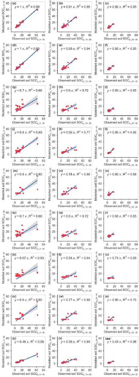
FIGURE 1. Comparison of the modeled and observed potential SOC (g kg−1) for (A–C) RFM, (D–F) GBRM, (G–I) MLRM, (J–L) SVMM, (M–O) RRTM, (P–R) ANNM, (S–U) GLRM, (V–X) CITM, and (Y–AA) eXGBM. The solid lines are the linear regression lines between the modeled and observed potential SOC. RFM, random forest models; GBRM, generalized boosted regression; MLRM, multiple linear regression model; SVMM, support vector machine model; RRTM, recursive regression tree model; ANNM, artificial neural network; GLRM, generalized linear regression model; CITM, conditional inference tree; eXGBM, eXtreme gradient boosting.
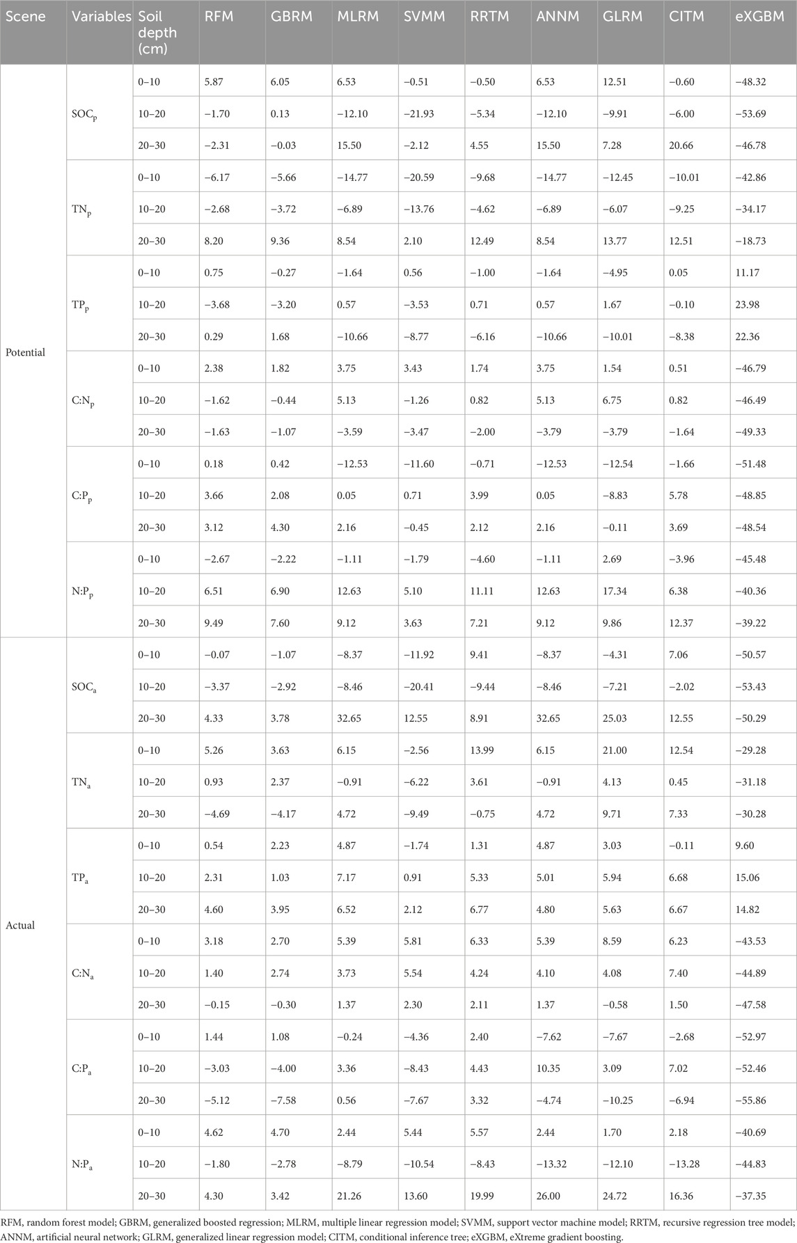
TABLE 1. The relative bias (unit, %) between modeled and observed soil carbon, nitrogen, and phosphorus and their ratios.
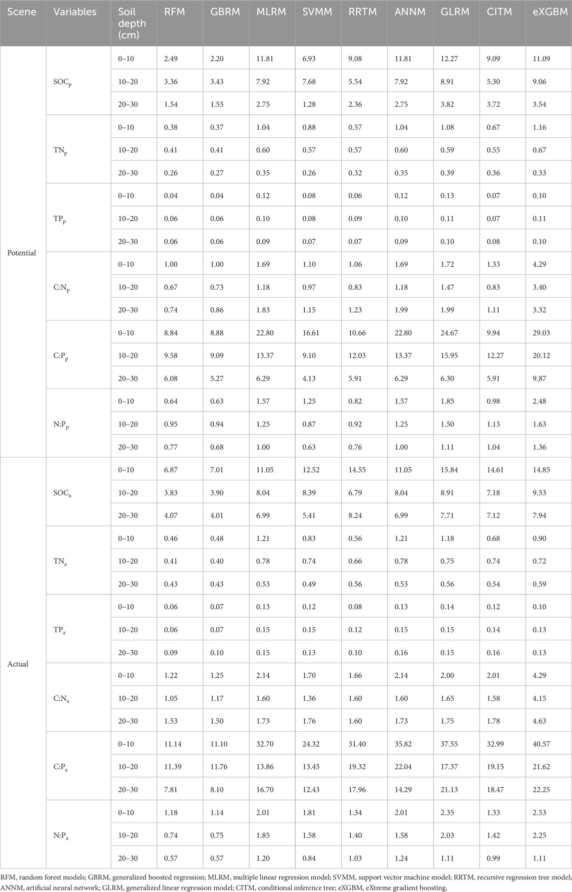
TABLE 2. The RMSE (unit, g kg−1 for SOC, TN, and TP) between modeled and observed soil carbon, nitrogen, and phosphorus and their ratios.
The RFM had the first highest accuracy among the nine models for the observed SOCa_0–10 and SOCa_10–20, whereas the GBRM had the second highest accuracy among the nine models for observed SOCa_0–10 and SOCa_10–20 (Figure 2; Tables 1, 2). By contrast, the RFM and GBRM were the second and first most accurate among the nine models for observed SOCa_20–30, respectively (Figure 2; Tables 1, 2). The linear slopes between the observed SOCa_0–10 (SOCa_10–20) and modeled SOCa_0–10 (SOCa_10–20) from the RFM and GBRM were 0.98 (≥0.91), but those from the other seven models were 1.10 or ≤0.84 (≤0.77) (Figure 2). The RMSEs between the observed SOCa_0–10 (SOCa_10–20) and modeled SOCa_0–10 (SOCa_10–20) from the RFM and GBRM were ≤7.01 g kg−1 (≤3.90 g kg−1), but those from the other seven models were ≥11.05 g kg−1 (≥6.79 g kg−1) (Table 2). The absolute values of relative bias between the observed SOCa_0–10 and modeled SOCa_0–10 from the RFM and GBRM were ≤1.07%, but those from the other seven models were ≥4.31% (Table 1). Modeled SOCa_0–10 from the RFM, GBRM, and eXGBM explained (R2=0.94) most of the variation in the observed SOCa_0–10, but that from the other six models only explained ≤84% of the variation in the observed SOCa_0–10 (Figure 2). The absolute values of relative bias between the observed SOCa_10–20 and modeled SOCa_10–20 from the CITM, GBRM, and RFM were the first (2.02%), second (2.92%), and third (3.37%) minimums, respectively, but those from the other six models were ≥7.21% (Table 1). However, the modeled SOCa_10–20 from the CITM, GBRM, and RFM explained 81%, 94%, and 100% of the variation in the observed SOCa_10–20, respectively (Figure 2). The linear slopes between the observed SOCa_20–30 and modeled SOCa_20–30 from the RFM, GBRM, MLRM, SVMM, and ANNM were ≥0.94, but those from the other four models were ≤0.84 (Figure 2). However, the RMSE and absolute values of relative bias between the observed SOCa_20–30 and modeled SOCa_20–30 from the RFM and GBRM were ≤4.07 g kg−1 and ≤4.33%, respectively, but those from the other seven models were ≥5.40 g kg−1 and ≥8.90%, respectively (Tables 1, 2). Modeled SOCa_20–30 from the RFM and GBRM explained 91% of the variation in the observed SOCa_20–30 but that from the other seven models only explained ≤88% of the variation (Figure 2).
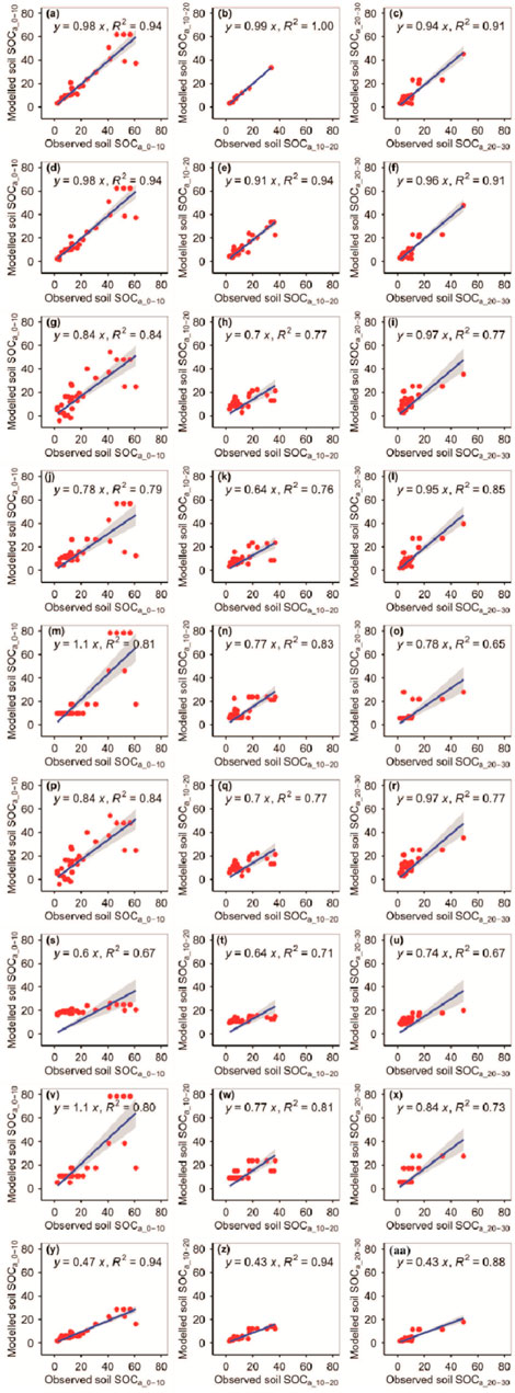
FIGURE 2. Comparison of the modeled and observed actual SOC (g kg−1) for (A–C) RFM, (D–F) GBRM, (G–I) MLRM, (J–L) SVMM, (M–O) RRTM, (P–R) ANNM, (S–U) GLRM, (V–X) CITM, and (Y–AA) eXGBM. The solid lines are the linear regression lines between the modeled and observed actual SOC. The abbreviations are the same as in Figure 1.
The RFM and GBRM were the second and first most accurate of the nine models for observed TNp_0–10, respectively (Figure 3; Tables 1, 2). By contrast, the RFM was the most accurate of the nine models for observed TNp_10–20 and TNp_20–30, whereas the GBRM was the second most accurate for observed TNp_10–20 and TNp_20–30 (Figure 3; Tables 1, 2). Modeled TNp_0–10, TNp_10–20, and TNp_20–30 from the RFM and GBRM explained 98%, 93%, and 93% of the variation in the observed TNp_0–10, TNp_10–20, and TNp_20–30, but those from the other seven models explained ≤96%, ≤92%, and ≤92% of the variation in the observed TNp_0–10, TNp_10–20, and TNp_20–30, respectively (Figure 3). The linear slopes between the observed TNp_0–10 and TNp_10–20 and modeled TNp_0–10 and TNp_10–20 from the RFM and GBRM were ≥0.89, but those from the other seven models were ≤0.85 (Figure 3). The absolute values of relative bias between the observed TNp_0–10 (TNp_10–20) and modeled TNp_0–10 (TNp_10–20) from the RFM and GBRM were ≤6.17% (≤3.72%), but those from the other seven models were ≥9.68% (≥4.62%) (Table 1). The RMSEs between the observed TNp_0–10 and TNp_10–20 and modeled TNp_0–10 and TNp_10–20 from the RFM and GBRM, respectively, were ≤0.41 g kg−1, but those from the other seven models were ≥0.55 g kg−1 (Table 2). The absolute value of relative bias between the observed TNp_20–30 and modeled TNp_20–30 from the RFM, GBRM, MLRM, SVMM, and ANNM was ≤9.36%, but that from the other four models was ≥12.49% (Table 1). However, the RMSEs between the observed TNp_20–30 and modeled TNp_20–30 from the RFM, GBRM, and SVMM were ≤0.27 g kg−1, and those from the other six models were ≥0.32 g kg−1 (Table 2). Moreover, the linear slopes between the observed TNp_20–30 and modeled TNp_20–30 from the RFM, GBRM, and RRTM were 1.00, but those from the other six models were ≤0.98 (Figure 3).
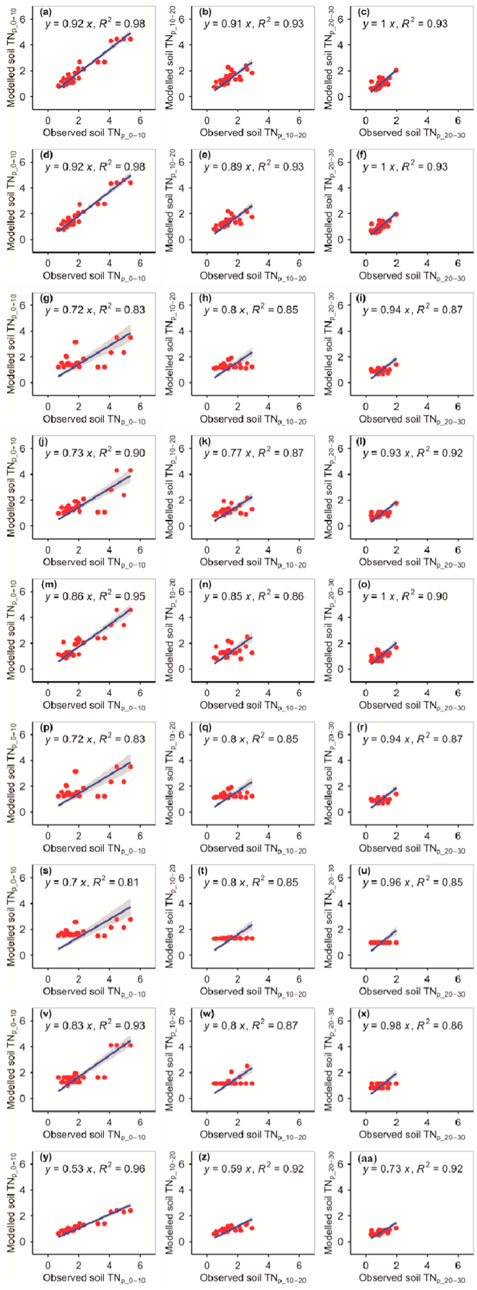
FIGURE 3. Comparison of the modeled and observed potential TN (g kg−1) for (A–C) RFM, (D–F) GBRM, (G–I) MLRM, (J–L) SVMM, (M–O) RRTM, (P–R) ANNM, (S–U) GLRM, (V–X) CITM, and (Y–AA) eXGBM. The solid lines are the linear regression lines between the modeled and observed potential TN. The abbreviations are the same as in Figure 1.
The RFM and GBRM were more accurate than the other seven models for the observed TNa_0–10, TNa_10–20, and TNa_20–30 (Figure 4; Tables 1, 2). The linear slopes between the observed TNa_0–10 and modeled TNa_0–10 from the RFM, GBRM, and RRTM were ≥0.94, but those from the other six models were ≤0.92 (Figure 4). However, the modeled TNa_0–10 from the RFM, GBRM, and RRTM explained ≥91% of the variation in the observed TNa_0–10, and those from the other six models explained ≤89% of the variation in the observed TNa_0–10 (Figure 4). The RMSEs between the observed TNa_0–10 and modeled TNa_0–10 from the RFM, GBRM, and RRTM were ≤0.56 g kg−1, but those from the other six models were ≥0.68 g kg−1 (Table 2). The absolute values of relative bias between the observed TNa_0–10 and modeled TNa_0–10 from the RFM, GBRM, and RRTM were 5.26%, 3.63%, and 13.99%, respectively (Table 1). The linear slopes between the observed TNa_10–20 and modeled TNa_10–20 from the RFM and GBRM were ≥0.91, but those from the other seven models were ≤0.86 (Figure 4). The modeled TNa_10–20 from the RFM and GBRM explained ≥92% of the variation in the observed TNa_10–20, and those from the other seven models explained ≤86% of the variation in the observed TNa_10–20 (Figure 4). The RMSE value between the observed TNa_10–20/TNa_20–30 and modeled TNa_10–20/TNa_20–30 from the RFM and GBRM was ≤0.43 g kg−1, but that from the other seven models was ≥0.49 g kg−1 (Table 2). The absolute values of relative bias between the observed TNa_10–20 and modeled TNa_10–20 from the RFM and GBRM were ≤2.37% (Table 1). The absolute values of relative bias between the observed TNa_20–30 and modeled TNa_20–30 from the RFM, GBRM, and RRTM were 4.69%, 4.17%, and 0.75%, respectively, but those from the other six models was ≥4.72% (Table 1). The modeled TNa_20–30 from the RFM, GBRM, and eXGBM could explain 89%, 88%, and 88% of the variation in the observed TNa_20–30, respectively, but those from the other six models explained ≤86% of the variation in the TNa_20–30 (Figure 4).
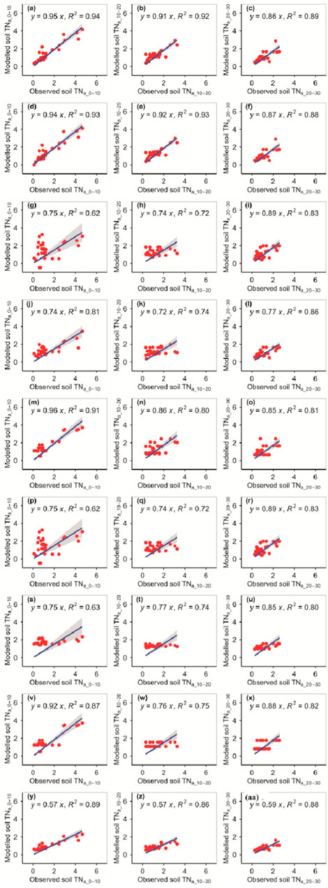
FIGURE 4. Comparison of the modeled and observed actual TN (g kg−1) for (A–C) RFM, (D–F) GBRM, (G–I) MLRM, (J–L) SVMM, (M–O) RRTM, (P–R) ANNM, (S–U) GLRM, (V–X) CITM, and (Y–AA) eXGBM. The solid lines are the linear regression lines between the modeled and observed actual TN. The abbreviations are the same as in Figure 1.
The RFM and GBRM were more accurate than the other seven models for observed TPp_0–10, TPp_10–20, and TPp_20–30 (Figure 5; Tables 1, 2). The RMSEs between the observed TPp_0–10, TPp_10–20, and TPp_20–30 and modeled TPp_0–10 (TPp_10–20) from the RFM and GBRM were 0.04, 0.06, and 0.06 g kg−1, respectively, but those from the other seven models were ≥0.06, 0.07, and 0.07 g kg−1 (Table 2). The modeled TPp_0–10 (TPp_10–20) from the RFM and GBRM explained 99% (≥97%) of the variation in the observed TPp_0–10 (TPp_10–20), but that from the other seven models explained ≤98% (≤96%) of the variation in the observed TPp_0–10 (TPp_10–20) (Figure 5). The modeled TPp_20–30 from the RFM, GBRM, and SVMM explained 97% of the variation in the observed TPp_20–30, but that from the other six models explained ≤96% of the variation in the observed TPp_20–30 (Figure 5). The absolute value of relative bias between the observed TPp_0–10 and modeled TPp_0–10 from the RFM, GBRM, SVMM, and CITM was ≤0.75%, but that from the other five models was ≥1.00% (Table 1). The absolute values of relative bias between the observed TPp_10–20 and modeled TPp_10–20 from the RFM, GBRM, MLRM, SVMM, RRTM, ANNM, GLRM, CITM, and eXGBM were 3.68%, 3.20%, 0.57%, 3.53%, 0.71%, 0.57%, 1.67%, 0.10%, and 23.98%, respectively (Table 1). The absolute values of relative bias between the observed TPp_20–30 and modeled TPp_20–30 from the RFM and GBRM were 0.29% and 1.68%, respectively, but that from the other seven models was ≥6.16% (Table 1). The linear slopes between the observed TPp_20–30 and modeled TPp_20–30 from the RFM and GBRM were 0.99 and 1.00, respectively, but those from the other seven models were 1.20 or ≤0.91 (Figure 5).
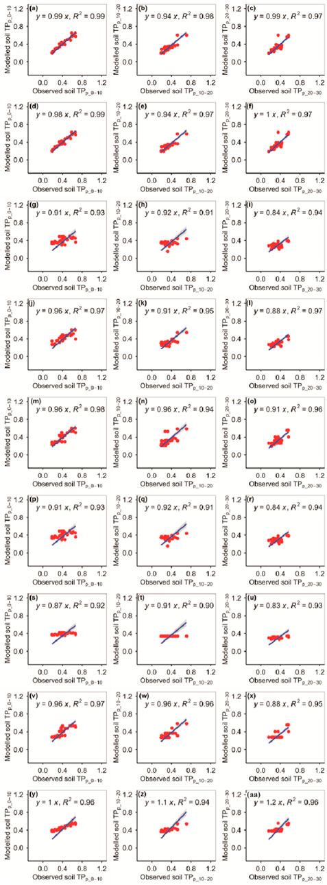
FIGURE 5. Comparison of modeled and observed potential TP (g kg−1) for (A–C) RFM, (D–F) GBRM, (G–I) MLRM, (J–L) SVMM, (M–O) RRTM, (P–R) ANNM, (S–U) GLRM, (V–X) CITM, and (Y–AA) eXGBM. The solid lines are the linear regression lines between the modeled and observed potential TP. The abbreviations are the same as in Figure 1.
The RFM and GBRM were more accurate than the other seven models at predicting TPa_0–10, TPa_10–20, and TPa_20–30 (Figure 6; Tables 1, 2). The absolute values of relative bias between the observed TPa_0–10, TPa_10–20, or TPa_20–30 and modeled TPa_0–10, TPa_10–20, or TPa_20–30 from the eXGBM were much greater than those of the other eight models (Table 1). There was an obvious phenomenon in which several observed TPa_0–10, TPa_10–20, or TPa_20–30 values corresponded to one modeled TPa_0–10, TPa_10–20, or TPa_20–30 value from the CITM, respectively (Figure 6). There was an obvious phenomenon in which several observed TPa_10–20 or TPa_20–30 values corresponded to one modeled TPa_10–20 or TPa_20–30 value from the ANNM, respectively (Figure 6). There was an obvious phenomenon in which several observed TPa_10–20 values corresponded to one modeled TPa_10–20 value from the GLRM, respectively (Figure 6). The RMSEs between the observed TPa_0–10 or TPa_10–20 and modeled TPa_0–10 or TPa_10–20 from the RFM and GBRM were ≤0.07 g kg−1, but those from the other seven models were ≥0.08 g kg−1 (Table 2). The modeled TPa_0–10 from the RFM, GBRM, and RRTM explained ≥97% of the variation in the observed TPa_0–10, but those from the other six models explained ≥95% of the variation in the observed TPa_0–10 (Figure 6). The linear slope and absolute value of relative bias between the observed TPa_0–10 and modeled TPa_0–10 from the RFM, GBRM, and RRTM were ≥0.98 and ≤2.23%, respectively (Figure 6; Table 1). The modeled TPa_10–20 from the RFM and GBRM explained 98% of the variation in the TPa_10–20, but those from the other seven models only explained ≤93% of the variation in TPa_10–20 (Figure 2). The relative bias and linear slope between the observed TPa_10–20 and modeled TPa_10–20 from the RFM and GBRM were 2.31% and 0.99, and 1.03% and 0.97, respectively (Table 1). The linear slope between the observed TPa_20–30 and modeled TPa_20–30 from the RFM, GBRM, RRTM, and eXGBM was 1.00, but that from the other five models was ≤0.95 (Figure 6). The modeled TPa_20–30 from the RFM, GBRM, and RRTM explained ≥95% of the variation in the observed TPa_20–30, but that from the other six models could only explain ≤92% of the variation in the observed TPa_20–30 (Figure 6). The RMSE between the observed TPa_20–30 and modeled TPa_20–30 from the RFM, GBRM, and RRTM was ≤0.10 g kg−1, but that from the other six models was ≥0.13 g kg−1 (Table 2). The absolute value of relative bias between the observed TPa_20–30 and modeled TPa_20–30 from the RFM, GBRM, and SVMM was ≤4.60%, but that from the other six models was ≥4.80% (Table 1).
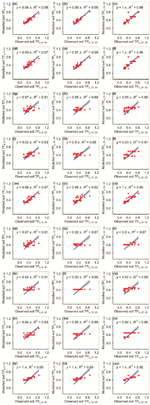
FIGURE 6. Comparison of the modeled and observed actual TP (g kg−1) for (A–C) RFM, (D–F) GBRM, (G–I) MLRM, (J–L) SVMM, (M–O) RRTM, (P–R) ANNM, (S–U) GLRM, (V–X) CITM, and (Y–AA) eXGBM. The solid lines are the linear regression lines between the modeled and observed actual TP. The abbreviations are the same as in Figure 1.
The RFM and GBRM were more accurate than the other seven models at predicting the C:Np_0–10, C:Np_10–20, and C:Np_20–30 (Figure 7; Tables 1, 2). The absolute values of relative bias between the observed C:Np_0–10, C:Np_10–20, or C:Np_20–30 and modeled C:Np_0–10, C:Np_10–20, or C:Np_20–30 from the eXGBM were much greater than those from the other eight models (Table 1). There was an obvious phenomenon in which several observed C:Np_0–10, C:Np_10–20, or C:Np_20–30 values corresponded to one modeled C:Np_0–10, C:Np_10–20, or C:Np_20–30 value from the RRTM, ANNM, and GLRM, respectively (Figure 7). Additionally, there was an obvious phenomenon in which several observed C:Np_0–10 or C:Np_10–20 values corresponded to one modeled C:Np_0–10 or C:Np_10–20 value from the CITM, respectively (Figure 7). The RMSEs between the observed C:N and modeled C:N from the RFM and GBRM at 0–10, 10–20, and 20–30 cm were 1.00, ≤0.73, and ≤0.86, but those from the other seven models were ≥1.06, ≥0.83, and ≥1.11, respectively (Table 2). The relative biases between the observed C:Np_0–10 and modeled C:Np_0–10 from the RFM, GBRM, MLRM, and SVMM were 2.38%, 1.82%, 3.75%, and 3.43%, respectively (Table 1). The relative biases between the observed C:Np_10–20 and modeled C:Np_10–20 from the RFM, GBRM, MLRM and SVMM were −1.62%, −0.44%, 5.13%, and −1.26%, respectively (Table 1). The absolute values of relative bias between the observed C:Np_20–30 and modeled C:Np_20–30 from the RFM and GBRM were ≤1.63%, but those from the other seven models w ≥1.64% (Table 1). The linear slope between the observed C:Np_20–30 and modeled C:Np_20–30 from the RFM and GBRM was 0.97, but that from the other seven models was ≤0.94 (Figure 7). The modeled C:Np_20–30 from the RFM and GBRM explained ≥98% of the variation in the observed C:Np_20–30, but that from the other seven models only explained ≤97% of the variation in C:Np_20–30 (Figure 7).

FIGURE 7. Comparison of the modeled and observed potential C:N for (A–C) RFM, (D–F) GBRM, (G–I) MLRM, (J–L) SVMM, (M–O) RRTM, (P–R) ANNM, (S–U) GLRM, (V–X) CITM, and (Y–AA) eXGBM. The solid lines are the linear regression lines between the modeled and observed potential C:N. The abbreviations are the same as in Figure 1.
The RFM was more accurate than the other eight models in predicting the C:Na_10–20 (Figure 8; Tables 1, 2). The RFM and GBRM were more accurate than the other seven models at predicting the C:Na_0–10 and C:Na_20–30 (Figure 8; Tables 1, 2). The absolute values of relative bias between the observed C:Na_0–10, C:Na_10–20, or C:Na_20–30 and modeled C:Na_0–10, C:Na_10–20, or C:Na_20–30, respectively, from the eXGBM were much greater than those from the other eight models (Table 1). There was an obvious phenomenon in which several observed C:Na_0–10, C:Na_10–20, or C:Na_20–30 values corresponded to one modeled C:Na_0–10, C:Na_10–20, or C:Na_20–30 value from the RRTM and CITM, respectively (Figure 8). Additionally, there was an obvious phenomenon in which several observed C:Na_10–20 values corresponded to one modeled C:Na_10–20 value from the ANNM (Figure 8). The absolute values of relative bias between the observed C:Na and modeled C:Na from the RFM and GBRM at 0–10, 10–20, and 20–30 cm were ≤3.18%, ≤2.74%, and ≤0.30%, but those from the other seven models were ≥5.39%, ≥3.73%, and ≥0.58%, respectively (Table 1). The RMSEs between the observed C:Na and modeled C:Na from the RFM and GBRM at 0–10, 10–20, and 20–30 cm were ≤1.25, ≤1.17, and ≤1.53, but those from the other seven models were ≥1.66, ≥1.36, and ≥1.60, respectively (Table 2).
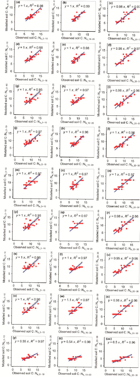
FIGURE 8. Comparison of the modeled and observed actual C:N for (A–C) RFM, (D–F) GBRM, (G–I) MLRM, (J–L) SVMM, (M–O) RRTM, (P–R) ANNM, (S–U) GLRM, (V–X) CITM, and (Y–AA) eXGBM. The solid lines are the linear regression lines between the modeled and observed actual C:N. The abbreviations are the same as in Figure 1.
The RFM and GBRM were more accurate than the other seven models in predicting the C:Pp_0–10, C:Pp_10–20, and C:Pp_20–30 (Figure 9; Tables 1, 2). The absolute value of relative bias between the observed C:Pp_0–10, C:Pp_10–20, or C:Pp_20–30 and modeled C:Pp_0–10, C:Pp_10–20, or C:Pp_20–30, respectively, from the eXGBM was much greater than those from the other eight models (Table 1). There was an obvious phenomenon in which several observed C:Pp_0–10, C:Pp_10–20, or C:Pp_20–30 values corresponded to one modeled C:Pp_0–10, C:Pp_10–20, or C:Pp_20–30 value from the GLRM and CITM, respectively (Figure 9). Both the linear slope and R2 values between the observed C:Pp_0–10 or C:Pp_10–20 and modeled C:Pp_0–10 or C:Pp_10–20 from the MLRM and ANNM were lower than 0.90, respectively (Figure 9). The RMSEs between the observed C:Pp_0–10 and modeled C:Pp_0–10 from the RFM and GBRM were ≤8.88, but those from the other seven models were ≥9.91 (Table 2). The absolute values of relative bias between the observed C:Pp_0–10 and modeled C:Pp_0–10 from the RFM and GBRM were ≤0.42%, but those from the other seven models were ≥0.71% (Table 1). The RMSEs between the observed C:Pp_10–20 and modeled C:Pp_10–20 from the RFM, GBRM, and SVMM were ≤9.58, but those from the other six models were ≥12.03 (Table 2). The linear slopes and R2 values between the observed C:Pp_10–20 and modeled C:Pp_10–20 from the RFM, GBRM, and SVMM were 1.00 and 0.94, 1.00 and 0.95, and 0.95 and 0.95, respectively (Figure 9). The RMSEs between the observed C:Pp_20–30 and modeled C:Pp_20–30 from the RFM, GBRM, SVMM, RRTM, and CITM were ≤6.08, but those from the other four models were ≥6.29 (Table 2). The linear slopes between the observed C:Pp_20–30 and modeled C:Pp_20–30 from the RFM, GBRM, SVMM, RRTM, and CITM were 0.98, 0.99, 0.95, 0.96, and 0.94, respectively (Figure 9).
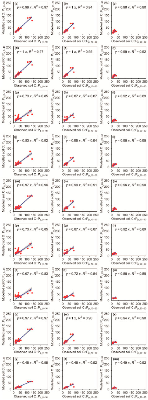
FIGURE 9. Comparison of the modeled and observed potential C:P for (A–C) RFM, (D–F) GBRM, (G–I) MLRM, (J–L) SVMM, (M–O) RRTM, (P–R) ANNM, (S–U) GLRM, (V–X) CITM, and (Y–AA) eXGBM. The solid lines are the linear regression lines between the modeled and observed potential C:P. The abbreviations are the same as in Figure 1.
The RFM was more accurate than the other eight models at predicting the C:Pa_10–20 (Figure 10; Tables 1, 2). The RFM and GBRM were more accurate than the other seven models at predicting the C:Pa_0–10 and C:Pa_20–30 (Figure 10; Tables 1, 2). The absolute values of relative bias between the observed C:Pa_0–10, C:Pa_10–20, or C:Pa_20–30 and modeled C:Pa_0–10, C:Pa_10–20, or C:Pa_20–30, respectively, from the eXGBM were much greater than those from the other eight models (Table 1). There was an obvious phenomenon in which several observed C:Pa_0–10, C:Pa_10–20, or C:Pa_20–30 values corresponded to one modeled C:Pa_0–10, C:Pa_10–20, or C:Pa_20–30 value from the RRTM, ANNM, and CITM, respectively (Figure 10). Linear slopes and R2 values between the observed C:Pa_0–10, C:Pa_10–20, or C:Pa_20–30 and modeled C:Pa_0–10, C:Pa_10–20, or C:Pa_20–30 from the GLRM were lower than 0.80 (Figure 10). Linear slopes between the observed C:Pa_0–10 or C:Pa_20–30 and modeled C:Pa_0–10 or C:Pa_20–30 from the MLRM and SVMM were also lower than 0.80, but those from the RFM and GBRM were ≥0.93 (Figure 10). The RMSEs between the observed C:Pa and modeled C:Pa from the RFM and GBRM were ≤11.76, but those from the other seven models were ≥12.43 (Table 2).
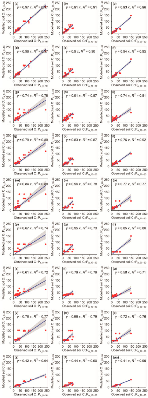
FIGURE 10. Comparison of the modeled and observed actual C:P for (A–C) RFM, (D–F) GBRM, (G–I) MLRM, (J–L) SVMM, (M–O) RRTM, (P–R) ANNM, (S–U) GLRM, (V–X) CITM, and (Y–AA) eXGBM. The solid lines are the linear regression lines between the modeled and observed actual C:P. The abbreviations are the same as in Figure 1.
The accuracy of the N:Pp_0–10, N:Pp_10–20, and N:Pp_20–30 also changed with different models (Figure 11; Tables 1, 2). The absolute values of relative bias between the observed N:Pp_0–10, N:Pp_10–20, or N:Pp_20–30 and modeled N:Pp_0–10, N:Pp_10–20, or N:Pp_20–30, respectively, from the eXGBM were much greater than those from the other eight models (Table 1). There was an obvious phenomenon in which several observed N:Pp_0–10, N:Pp_10–20, or N:Pp_20–30 values corresponded to one modeled N:Pp_0–10, N:Pp_10–20, or N:Pp_20–30 value from the GLRM and CITM, respectively (Figure 11). The RMSEs between the observed N:Pp_0–10 and modeled N:Pp_0–10 from the RFM and GBRM were ≤0.64, but those from the other seven models were ≥0.82 (Table 2). The RMSEs between the observed N:P and modeled N:P from the RFM, GBRM, SVMM, and RRTM at 10–20 cm and 20–30 cm were ≤0.95 and ≤0.77, but those from the other five models were ≥1.13 and ≥1.00, respectively (Table 2). However, the linear slopes between the observed N:Pp_10–20 and modeled N:Pp_10–20 from the RFM, GBRM, SVMM, and RRTM were 1.00, 1.00, 0.98, and 1.10, respectively (Figure 11).
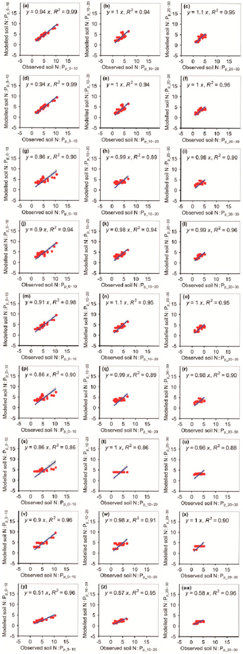
FIGURE 11. Comparison of modeled and observed potential N:P for (A–C) RFM, (D–F) GBRM, (G–I) MLRM, (J–L) SVMM, (M–O) RRTM, (P–R) ANNM, (S–U) GLRM, (V–X) CITM, and (Y–AA) eXGBM. The solid lines are the linear regression lines between the modeled and observed potential N:P. The abbreviations are the same as in Figure 1.
The RFM was more accurate than the other eight models in predicting N:Pa_10–20 (Figure 12; Tables 1, 2). The RFM and GBRM were more accurate than the other seven models at predicting N:Pa_0–10 and N:Pa_20–30 (Figure 12; Tables 1, 2). The absolute values of relative bias between the observed N:Pa_0–10, N:Pa_10–20, or N:Pa_20–30 and modeled N:Pa_0–10, N:Pa_10–20, or N:Pa_20–30, respectively, from the eXGBM were much greater than the other eight models, respectively (Table 1). The absolute values of relative bias between the observed N:Pa_0–10 and modeled N:Pa_0–10 from the MLRM, ANNM, GLRM, and CITM were lower than those from the RFM and GBRM (Table 1). However, there was an obvious phenomenon in which several observed N:Pa_0–10 values corresponded to one modeled N:Pa_0–10 from the CITM (Figure 12). The RMSEs between the observed N:Pa and modeled N:Pa from the RFM and GBRM at 0–10 cm, 10–20 cm, and 20–30 cm were ≤1.18, ≤0.75, and 0.57, but those from the other seven models were ≥1.33, ≥1.40, and ≥0.84, respectively (Table 2). The modeled N:Pa from the RFM and GBRM explained ≥94%, 97%, and 95% of the variation in the observed N:Pa at 0–10 cm, 10–20 cm, and 20–30 cm, respectively, but those from the other seven models only explained ≤93%, ≤94%, and ≤93% of the variation in the observed N:Pa (Figure 12). The slopes between the observed N:Pa and modeled N:Pa from the RF and GBRM at 0–10 cm and 10–20 cm were ≥0.95, but those from the other seven models were ≤0.93 (Figure 12). The slopes between the observed N:Pa_20–30 and modeled N:Pa_20–30 from the RF and GBRM were 1.00 and 0.99, respectively (Figure 12). The absolute values of relative bias between the observed N:Pa and modeled N:Pa from the RFM and GBRM at 10–20 cm and 20–30 cm were ≤4.30%, but those from the other seven models were ≥8.43% (Table 1).
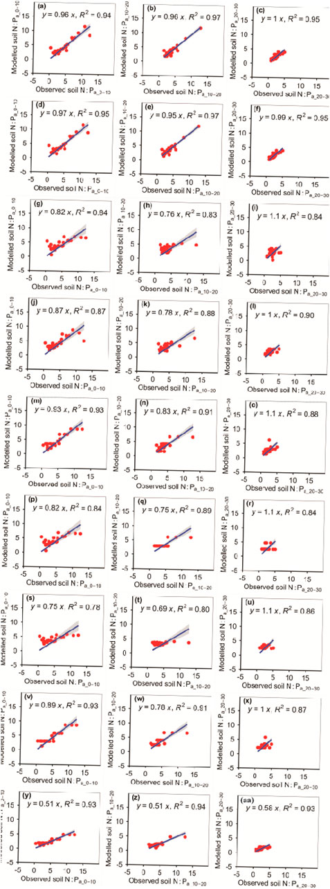
FIGURE 12. Comparison of the modeled and observed actual N:P for (A–C) RFM, (D–F) GBRM, (G–I) MLRM, (J–L) SVMM, (M–O) RRTM, (P–R) ANNM, (S–U) GLRM, (V–X) CITM, and (Y–AA) eXGBM. The solid lines are the linear regression lines between the modeled and observed actual N:P. The abbreviations are the same as in Figure 1.
Overall, the ARad, AP and AT based on the RFM explained the most variation in SOC, TN, TP, C:N, C:P, and N:P, those based on the RRTM explained the second most variation, and those based on the MLRM explained the least variation under the non-grazing scenarios (Supplementary Tables S1, S3, S5). The ARad, AP, AT, and NDVImax based on the RFM explained the most variation in SOC, TN, TP, C:N, C:P, and N:P, those based on the RRTM explained the second most variation, and those based on the MLRM explained the least variation under the free-grazing scenarios (Supplementary Tables S1, S3, S5). That is, the RFM had a greater ability to explain the six soil variables than the RRTM and MLRM, whereas the RRTM had a greater ability to explain the six soil variables than the MLRM. This finding supported some previous studies that demonstrated that the RFM had a greater ability to explain soil moisture and pH, plant species α-diversity, forage nutrition quality, and storage (Han et al., 2022; Tian and Fu, 2022; Dai et al., 2023; Wang and Fu, 2023). Moreover, the prediction accuracy of RFM was also higher than that of RRTM and MLRM (Tables 1, 2). This finding also supported some previous studies that demonstrated that the RFM had a higher prediction accuracy of soil moisture and pH, plant species α-diversity, forage nutrition quality, and storage than the RRTM and MLRM in grasslands on the Tibetan Plateau (Han et al., 2022; Tian and Fu, 2022; Dai et al., 2023; Wang and Fu, 2023). Therefore, the performance of the RFM was better than the RRTM and MLRM, at least for the grassland areas on the Xizang Plateau.
The R2 values under the non-grazing scenarios were not always lower than those under the free-grazing scenarios when we constructed the models of the six soil variables (Supplementary Tables S1, S3, S5). Moreover, the model accuracies under the non-grazing scenarios were not always lower than those under the free-grazing scenarios (Tables 1, 2). This finding implied that the increase in the number of independent variables cannot always improve the accuracy of the models. This finding was similar to several previous studies conducted on (Han et al., 2022; Tian and Fu, 2022; Dai et al., 2023; Wang and Fu, 2023) and outside the Qinghai-Xizang Plateau (Veloso et al., 2022). These previous studies found that the numbers of the input variables were not always positively related to the model accuracies of soil moisture and pH, plant species α-diversity, forage nutrition quality, and storage (Han et al., 2022; Tian and Fu, 2022; Dai et al., 2023; Wang and Fu, 2023). Moreover, a previous study found that the R2 value (<0.86) between the observed and modeled SOC pool in a previous study (Liu et al., 2023) was lower than that between the observed and modeled SOC in this study, but the input variables numbers (>=12) of the previous study (Liu et al., 2023) were much greater than those in this study. Therefore, an increase in the input variables of the model does not always lead to a better model of plant and soil variables, at least for the grasslands of the Xizang Plateau. Moreover, instead of focusing on increasing the number of input variables and how to obtain more accurate input variable data, it is better to focus on how to find the optimal model to better help solve related ecological and environmental problems.
Similar to some previous studies (Dai et al., 2023; Wang and Fu, 2023), the predicted accuracies of the six soil variables based on the RFM were dependent on soil depth. This finding may be due to the following mechanisms. First, soil moisture and pH can regulate their responses of SOC, TN, TP, C:N, C:P and N:P to external disturbance (e.g., warming) (Yu et al., 2019a). The predicted accuracies of the six soil variables should be related to those of soil moisture and soil pH. In addition, soil moisture and pH can generally change with soil depth. Second, solar radiation and precipitation first reach the surface of soils and then gradually reach the deep layer of soils through energy conduction or infiltration. The normalized difference vegetation index is calculated by the spectral information reflected by land surface, and the energy source of air temperature is mainly the long-wave radiation of the land surface. All of these may lead to closer relationships between the six topsoil variables and the four input variables than deeper soil variables.
The RFM and GBRM achieved a greater accuracy for the six soil variables than the other seven models. However, the tree numbers of the GBRM were much greater than those of the RFM for most cases (Supplementary Tables S1, S2). The model complexity can be generally positively correlated with the tree numbers, whereas the calculation speed can be generally negatively correlated with the tree numbers (Han et al., 2022; Tian and Fu, 2022). Therefore, the RFM should be the best model among the nine models when all things are considered in this study, which was in line with the hypothesis. This phenomenon was similar to some previous studies that demonstrated that the RFM performed better than the other models at modeling soil moisture and pH, plant species α-diversity, forage nutrition quality, and storage in grassland ecological systems on (Han et al., 2022; Tian and Fu, 2022; Dai et al., 2023; Wang and Fu, 2023) and outside the Qinghai-Xizang Plateau (Fernandez-Delgado et al., 2014; Nussbaum et al., 2018). All these findings further support the advantage of the RFM in modeling soil and plant variables in grasslands on the Qinghai-Xizang Plateau.
The prediction accuracy of the six variables based on the RFM was greater than those in some previous studies (Yang et al., 2008; Yang et al., 2009; Yang et al., 2010; Shangguan et al., 2013; Kou et al., 2019; Wang et al., 2020; Wang et al., 2021a; Liu et al., 2023). For example, the modeled TN could only explain 34%–41% of the variation in the observed TN, and the RMSEs and relative bias were 1.15–1.20 g kg−1 and 49.17% in China, respectively (Zhou et al., 2020). Moreover, compared with some previous studies (Kou et al., 2019; Wang et al., 2021a; Liu et al., 2023), although the number of independent variables used in the models constructed in this study was small, the accuracy was not reduced. This phenomenon may be due to the introduction of more independent variables that may introduce new uncertainties, considering that any independent variable can have its own data quality. Therefore, the RFM of SOC, TN, TP, C:N, C:P and N:P at the three depths in this study can have relative accuracies and can be used for related studies (e.g., the spatial distribution of these six variables) in grassland areas on the Xizang Plateau.
It is well known that climate change and human activities together affect these soil variables (Yu et al., 2019a; Zhang and Fu, 2021; Zha et al., 2022), but their relative contributions are unclear. Many previous studies only modeled actual soil organic carbon, total nitrogen, total phosphorus, and their ratios (Yang et al., 2009; Kou et al., 2019), so it was difficult to disentangle the relative effects of climate change and human activity on these soil variables. However, in this study, the potential and actual random forest models of these soil variables were constructed respectively, so it was relatively easy to separate the relative contributions of climate change and human activities to these soil variables.
There are some uncertainties or limitations in this study. First, as the NDVI comes from optical remote sensing, it is often affected by the conditions of satellite itself (such as instrument failure), the angle between the satellite remote sensing and the surface, weather conditions, and land surface conditions. The Xizang Plateau became dimming, which coincided with the increase in precipitation during 2000–2020 (Huang and Fu, 2023). During the rainy season on the Xizang Plateau, it is often rainy or cloudy for several consecutive days, which may prevent the collection of near infrared and red band data of plants and the calculation of the NDVI. On the Xizang Plateau, grassland productivity tends to decline from southeast to northwest. The NDVI is easy to saturate in areas with high vegetation productivity, while it is affected by soil interference in areas with low vegetation productivity (Ma et al., 2022; Shen et al., 2022). Second, many grassland areas on the Xizang Plateau have steep slopes, and the soil samples were mainly collected in areas with relatively shallow slopes. This may affect the relationships between these soil variables and climate data or NDVI data. Third, although climate and NDVI data are based on the corresponding year, soil variables are not entirely derived from observations in the same year, and climate change and human activities may alter these soil variables (Zhang et al., 2015; Fu and Shen, 2017). This phenomenon may also interfere with the model accuracy. Fourth, although the climate data used in this study can be highly accurate, there is some uncertainty associated with them. Fifth, only random forest models with soil variables at depths of 0–10, 10–20, and 20–30 cm were built in this study; therefore, future studies may consider building optimal models of soil variables at greater depths. Sixth, the data in this study were all obtained from the Xizang Plateau; therefore, it may be necessary to further test the accuracy of the models constructed in this study when extrapolating them to other regions of the Qinghai-Xizang Plateau. We can consider additional soil sampling in other areas of the plateau to build the optimal model of soil variables in the entire Qinghai-Xizang Plateau region in the future. Finally, only random forest models of the contents of these soil variables were constructed in this study, and the densities of soil organic carbon, total nitrogen, and total phosphorus could better reflect the changes in these soil variables. Therefore, the construction of optimal models of soil organic carbon density, total nitrogen density, and total phosphorus density should be considered in the future.
This study is the first to model SOC, TN, TP, C:N, C:P, and N:P at depths of 0–10, 10–20, and 20–30 cm under non-grazing and free-grazing scenarios based on nine methods. We can build a database of soil carbon, nitrogen, and phosphorus and their ratios over the past few decades or for the future across the whole grasslands of the Xizang Plateau under fencing and free-grazing conditions using the RFM established in this study. This database can be used to solve some of ecological, environmental, and soil management problems in grassland ecosystems in the Xizang Plateau. For example, the relative effects of climate change and human activities on soil organic carbon during the past decades can be distinguished and quantified, thus providing data support for improving soil carbon sequestration and mitigating climate warming.
The original contributions presented in the study are included in the article/Supplementary Material, further inquiries can be directed to the corresponding author.
SW: Writing–original draft, Writing–review and editing. HQ: Investigation, Writing–original draft. TL: Investigation, Writing–original draft. YQ: Investigation, Writing–original draft. GF: Conceptualization, Validation, Visualization, Writing–original draft, Writing–review and editing. XP: Writing–original draft. XZ: Writing–original draft.
The author(s) declare financial support was received for the research, authorship, and/or publication of this article. This study was funded by Henan Zhongmu County Research Project (E3C1050101), Remote Sensing Big data Analytics Project (E3E2051401), the Beijing Chaoyang District Collaborative Innovation Project (E2DZ050100), the Chinese Academy of Sciences Youth Innovation Promotion Association (2020054), National Natural Science Foundation of China (31600432), Tibet Autonomous Region Science and Technology Project (XZ202301YD0012C, XZ202202YD0009C, XZ202201ZY0003N, XZ202101ZD0007G, and XZ202101ZD0003N), and Construction of Zhongba County Fixed Observation and Experiment Station of First Support System for Agriculture Green Development.
The authors declare that the research was conducted in the absence of any commercial or financial relationships that could be construed as a potential conflict of interest.
The reviewer XS declared a shared affiliation with the authors SW, HQ, TL, YQ, and GF to the handling editor.
All claims expressed in this article are solely those of the authors and do not necessarily represent those of their affiliated organizations, or those of the publisher, the editors and the reviewers. Any product that may be evaluated in this article, or claim that may be made by its manufacturer, is not guaranteed or endorsed by the publisher.
The Supplementary Material for this article can be found online at: https://www.frontiersin.org/articles/10.3389/feart.2023.1340020/full#supplementary-material
Bahram, M., Espenberg, M., Pärn, J., Lehtovirta-Morley, L., Anslan, S., Kasak, K., et al. (2022). Structure and function of the soil microbiome underlying N2O emissions from global wetlands. Nat. Commu. 13, 1430. doi:10.1038/s41467-022-29161-3
Bangelesa, F., Adam, E., Knight, J., Dhau, I., Ramudzuli, M., and Mokotjomela, T. M. (2020). Predicting soil organic carbon content using hyperspectral remote sensing in a degraded mountain landscape in Lesotho. Appl. Environ. Soil Sci. 2020, 1–11. doi:10.1155/2020/2158573
Dai, E., Zhang, G., Fu, G., and Zha, X. (2023). Can meteorological data and normalized difference vegetation index be used to quantify soil pH in grasslands? Front. Ecol. Evol. 11. doi:10.3389/fevo.2023.1206581
de Melo, A. A. B., Valladares, G. S., Ceddia, M. B., Pereira, M. G., and Soares, I. (2016). Spatial distribution of organic carbon and humic substances in irrigated soils under different management systems in a semi-arid zone in Ceara, Brazil. Semina-Ciencias Agrar. 37, 1845–1855. doi:10.5433/1679-0359.2016v37n4p1845
Feng, D., Bao, W., and Pang, X. (2017). Consistent profile pattern and spatial variation of soil C/N/P stoichiometric ratios in the subalpine forests. J. Soil Sediment. 17, 2054–2065. doi:10.1007/s11368-017-1665-9
Fernandez-Delgado, M., Cernadas, E., Barro, S., and Amorim, D. (2014). Do we need hundreds of classifiers to solve real world classification problems? J. Mach. Learn. Res. 15, 3133–3181.
Fu, G., and Shen, Z. (2022). Asymmetrical warming of growing/non-growing season increases soil respiration during growing season in an alpine meadow. Sci. Total Environ. 812, 152591. doi:10.1016/j.scitotenv.2021.152591
Fu, G., Shen, Z., Zhang, X., Shi, P., Zhang, Y., and Wu, J. (2011). Estimating air temperature of an alpine meadow on the Northern Tibetan Plateau using MODIS land surface temperature. Acta Ecol. Sin. 31, 8–13. doi:10.1016/j.chnaes.2010.11.002
Fu, G., and Shen, Z. X. (2017). Response of alpine soils to nitrogen addition on the Tibetan Plateau: a meta-analysis. Appl. Soil Ecol. 114, 99–104. doi:10.1016/j.apsoil.2017.03.008
Fu, G., Shen, Z. X., Zhang, X. Z., Zhou, Y. T., and Zhang, Y. J. (2012). Response of microbial biomass to grazing in an alpine meadow along an elevation gradient on the Tibetan Plateau. Eur. J. Soil Biol. 52, 27–29. doi:10.1016/j.ejsobi.2012.05.004
Fu, G., Wang, J., and Li, S. (2022). Response of forage nutritional quality to climate change and human activities in alpine grasslands. Sci. Total Environ. 845, 157552. doi:10.1016/j.scitotenv.2022.157552
Ganjurjav, H., Gao, Q., Zhang, W., Liang, Y., Li, Y., Cao, X., et al. (2015). Effects of warming on CO2 fluxes in an alpine meadow ecosystem on the central Qinghai-Tibetan Plateau. PLoS ONE 10, e0132044. doi:10.1371/journal.pone.0132044
Han, F., Fu, G., Yu, C., and Wang, S. (2022). Modeling nutrition quality and storage of forage using climate data and normalized-difference vegetation index in alpine grasslands. Remote Sens. 14, 3410. doi:10.3390/rs14143410
Han, F., Yu, C., and Fu, G. (2023a). Non-growing/growing season non-uniform-warming increases precipitation use efficiency but reduces its temporal stability in an alpine meadow. Front. Plant Sci. 14, 1090204. doi:10.3389/fpls.2023.1090204
Han, F., Yu, C., and Fu, G. (2023b). Temperature sensitivities of aboveground net primary production, species and phylogenetic diversity do not increase with increasing elevation in alpine grasslands. Glob. Ecol. Conserv. 43, e02464. doi:10.1016/j.gecco.2023.e02464
Huang, S., and Fu, G. (2023). Impacts of climate change and human activities on plant species α-diversity across the Tibetan grasslands. Remote Sens. 15, 2947. doi:10.3390/rs15112947
Hutson, M. (2022). Taught to the test. Sci. (New York, N.Y.) 376, 570–573. doi:10.1126/science.abq7833
Kou, D., Ding, J., Li, F., Wei, N., Fang, K., Yang, G., et al. (2019). Spatially-explicit estimate of soil nitrogen stock and its implication for land model across Tibetan alpine permafrost region. Sci. Total Environ. 650, 1795–1804. doi:10.1016/j.scitotenv.2018.09.252
Kou, D., Yang, G., Li, F., Feng, X., Zhang, D., Mao, C., et al. (2020). Progressive nitrogen limitation across the Tibetan alpine permafrost region. Nat. Commu. 11, 3331. doi:10.1038/s41467-020-17169-6
Li, J., Gong, J., Guldmann, J.-M., Li, S., and Zhu, J. (2020). Carbon dynamics in the northeastern Qinghai-Tibetan Plateau from 1990 to 2030 using landsat land use/cover change data. Remote Sens. 12, 528. doi:10.3390/rs12030528
Li, S., Liu, Y., Lyu, S., Wang, S., Pan, Y., and Qin, Y. (2021). Change in soil organic carbon and its climate drivers over the Tibetan Plateau in CMIP5 earth system models. Theor. Appl. Climatol. 145, 187–196. doi:10.1007/s00704-021-03631-y
Liu, S., Sun, Y., Dong, Y., Zhao, H., Dong, S., Zhao, S., et al. (2019). The spatio-temporal patterns of the topsoil organic carbon density and its influencing factors based on different estimation models in the grassland of Qinghai-Tibet Plateau. PLoS ONE 14, e0225952. doi:10.1371/journal.pone.0225952
Liu, X., Zhou, T., Zhao, X., Shi, P., Zhang, Y., Xu, Y., et al. (2023). Patterns and drivers of soil carbon change (1980s-2010s) in the northeastern Qinghai-Tibet Plateau. Geoderma 434, 116488. doi:10.1016/j.geoderma.2023.116488
Ma, R., Shen, X., Zhang, J., Xia, C., Liu, Y., Wu, L., et al. (2022). Variation of vegetation autumn phenology and its climatic drivers in temperate grasslands of China. Int. J. Appl. Earth Obs. Geoinf. 114, 103064. doi:10.1016/j.jag.2022.103064
Marcal, M. F. M., Souza, Z. M. d., Tavares, R. L. M., Farhate, C. V. V., Oliveira, S. R. M., and Galindo, F. S. (2021). Predictive models to estimate carbon stocks in agroforestry systems. Forests 12, 1240. doi:10.3390/f12091240
Mikhailova, E. A., Bryant, R. B., DeGloria, S. D., Post, C. J., and Vassenev, (2000). Modeling soil organic matter dynamics after conversion of native grassland to long-term continuous fallow using the CENTURY model. Ecol. Model. 132, 247–257. doi:10.1016/s0304-3800(00)00273-8
Niu, B., and Fu, G. (2024). Response of plant diversity and soil microbial diversity to warming and increased precipitation in alpine grasslands on the Qinghai-Xizang Plateau - a review. Sci. Total Environ. 912, 168878. doi:10.1016/j.scitotenv.2023.168878
Nussbaum, M., Spiess, K., Baltensweiler, A., Grob, U., Keller, A., Greiner, L., et al. (2018). Evaluation of digital soil mapping approaches with large sets of environmental covariates. Soil 4, 1–22. doi:10.5194/soil-4-1-2018
Reichstein, M., Camps-Valls, G., Stevens, B., Jung, M., Denzler, J., Carvalhais, N., et al. (2019). Deep learning and process understanding for data-driven Earth system science. Nature 566, 195–204. doi:10.1038/s41586-019-0912-1
Shangguan, W., Dai, Y., Liu, B., Zhu, A., Duan, Q., Wu, L., et al. (2013). A China data set of soil properties for land surface modeling. J. Adv. Model. Earth Syst. 5, 212–224. doi:10.1002/jame.20026
Shen, X., Liu, B., Henderson, M., Wang, L., Jiang, M., and Lu, X. (2022). Vegetation greening, extended growing seasons, and temperature feedbacks in warming temperate grasslands of China. J. Clim. 35, 5103–5117. doi:10.1175/jcli-d-21-0325.1
Shit, P. K., Bhunia, G. S., and Maiti, R. (2016). Spatial analysis of soil properties using GIS based geostatistics models. Model. Earth Syst. Environ. 2, 107. doi:10.1007/s40808-016-0160-4
Sun, W., Li, S., Wang, J., and Fu, G. (2021). Effects of grazing on plant species and phylogenetic diversity in alpine grasslands, Northern Tibet. Ecol. Eng. 170, 106331. doi:10.1016/j.ecoleng.2021.106331
Tian, Y., and Fu, G. (2022). Quantifying plant species α-diversity using normalized difference vegetation index and climate data in alpine grasslands. Remote Sens. 14, 5007. doi:10.3390/rs14195007
Tornquist, C. G., Mielniczuk, J., and Cerri, C. E. P. (2009). Modeling soil organic carbon dynamics in oxisols of ibiruba (Brazil) with the century model. Soil till. Res. 105, 33–43. doi:10.1016/j.still.2009.05.005
Veloso, M. F., Rodrigues, L. N., and Fernandes, E. I. (2022). Evaluation of machine learning algorithms in the prediction of hydraulic conductivity and soil moisture at the Brazilian Savannah. Geoderma Reg. 30, e00569. doi:10.1016/j.geodrs.2022.e00569
Wang, D., Li, X., Zou, D., Wu, T., Xu, H., Hu, G., et al. (2020). Modeling soil organic carbon spatial distribution for a complex terrain based on geographically weighted regression in the eastern Qinghai-Tibetan Plateau. Catena 187, 104399. doi:10.1016/j.catena.2019.104399
Wang, D., Wu, T., Zhao, L., Mu, C., Li, R., Wei, X., et al. (2021a). A 1 km resolution soil organic carbon dataset for frozen ground in the Third Pole. Earth Syst. Sci. Data 13, 3453–3465. doi:10.5194/essd-13-3453-2021
Wang, J., Li, M., Yu, C., and Fu, G. (2022). The change in environmental variables linked to climate change has a stronger effect on aboveground net primary productivity than does phenological change in alpine grasslands. Front. Plant Sci. 12, 798633. doi:10.3389/fpls.2021.798633
Wang, J., Yu, C., and Fu, G. (2021b). Warming reconstructs the elevation distributions of aboveground net primary production, plant species and phylogenetic diversity in alpine grasslands. Ecol. Indic. 133, 108355. doi:10.1016/j.ecolind.2021.108355
Wang, S., and Fu, G. (2023). Modelling soil moisture using climate data and normalized difference vegetation index based on nine algorithms in alpine grasslands. Front. Environ. Sci. 11. doi:10.3389/fenvs.2023.1130448
Yang, Y., Fang, J., Ma, W., Smith, P., Mohammat, A., Wang, S., et al. (2010). Soil carbon stock and its changes in northern China's grasslands from 1980s to 2000s. Glob. Change Biol. 16, 3036–3047. doi:10.1111/j.1365-2486.2009.02123.x
Yang, Y. H., Fang, J., Smith, P., Tang, Y., Chen, A., Ji, C., et al. (2009). Changes in topsoil carbon stock in the Tibetan grasslands between the 1980s and 2004. Glob. Change Biol. 15, 2723–2729. doi:10.1111/j.1365-2486.2009.01924.x
Yang, Y. H., Fang, J., Tang, Y., Ji, C., Zheng, C., He, J., et al. (2008). Storage, patterns and controls of soil organic carbon in the Tibetan grasslands. Glob. Change Biol. 14, 1592–1599. doi:10.1111/j.1365-2486.2008.01591.x
Yang, Y. H., Ma, W. H., Mohammat, A., and Jing-Yun, F. (2007). Storage, patterns and controls of soil nitrogen in China. Pedosphere 17, 776–785. doi:10.1016/s1002-0160(07)60093-9
Yu, C. Q., Han, F. S., and Fu, G. (2019a). Effects of 7 years experimental warming on soil bacterial and fungal community structure in the Northern Tibet alpine meadow at three elevations. Sci. Total Environ. 655, 814–822. doi:10.1016/j.scitotenv.2018.11.309
Yu, C. Q., Wang, J. W., Shen, Z. X., and Fu, G. (2019b). Effects of experimental warming and increased precipitation on soil respiration in an alpine meadow in the Northern Tibetan Plateau. Sci. Total Environ. 647, 1490–1497. doi:10.1016/j.scitotenv.2018.08.111
Zha, X. J., Tian, Y., and Ouzhu Fu, G. (2022). Response of forage nutrient storages to grazing in alpine grasslands. Front. Plant Sci. 13, 991287. doi:10.3389/fpls.2022.991287
Zhang, H., and Fu, G. (2021). Responses of plant, soil bacterial and fungal communities to grazing vary with pasture seasons and grassland types, northern Tibet. Land Degrad. Dev. 32, 1821–1832. doi:10.1002/ldr.3835
Zhang, X. Z., Shen, Z. X., and Fu, G. (2015). A meta-analysis of the effects of experimental warming on soil carbon and nitrogen dynamics on the Tibetan Plateau. Appl. Soil Ecol. 87, 32–38. doi:10.1016/j.apsoil.2014.11.012
Zhang, Y., Tang, Y., Jiang, J., and Yang, Y. (2007). Characterizing the dynamics of soil organic carbon in grasslands on the Qinghai-Tibetan Plateau. Sci. China Ser. D. 50, 113–120. doi:10.1007/s11430-007-2032-2
Zhang, Y., Zhang, N., Yin, J., Yang, F., Zhao, Y., Jiang, Z., et al. (2020). Combination of warming and N inputs increases the temperature sensitivity of soil N2O emission in a Tibetan alpine meadow. Sci. Total Environ. 704, 135450. doi:10.1016/j.scitotenv.2019.135450
Zhao, X., Zhang, W., Feng, Y., Mo, Q., Su, Y., Njoroge, B., et al. (2022). Soil organic carbon primarily control the soil moisture characteristic during forest restoration in subtropical China. Front. Ecol. Evol. 10. doi:10.3389/fevo.2022.1003532
Zhou, Y., Xue, J., Chen, S., Liang, Z., Wang, N., and Shi, Z. (2020). Fine-resolution mapping of soil total nitrogen across China based on weighted model averaging. Remote Sens. 12, 85. doi:10.3390/rs12010085
Keywords: big data mining, random forest, global change, Tibetan plateau, alpine region
Citation: Wang S, Qi H, Li T, Qin Y, Fu G, Pan X and Zha X (2024) Can normalized difference vegetation index and climate data be used to estimate soil carbon, nitrogen, and phosphorus and their ratios in the Xizang grasslands?. Front. Earth Sci. 11:1340020. doi: 10.3389/feart.2023.1340020
Received: 17 November 2023; Accepted: 28 December 2023;
Published: 02 February 2024.
Edited by:
Shiv Prasad, Indian Agricultural Research Institute (ICAR), IndiaReviewed by:
Licong Dai, Hainan University, ChinaCopyright © 2024 Wang, Qi, Li, Qin, Fu, Pan and Zha. This is an open-access article distributed under the terms of the Creative Commons Attribution License (CC BY). The use, distribution or reproduction in other forums is permitted, provided the original author(s) and the copyright owner(s) are credited and that the original publication in this journal is cited, in accordance with accepted academic practice. No use, distribution or reproduction is permitted which does not comply with these terms.
*Correspondence: Gang Fu, ZnVnYW5nQGlnc25yci5hYy5jbg==, ZnVnYW5nMDlAMTI2LmNvbQ==
Disclaimer: All claims expressed in this article are solely those of the authors and do not necessarily represent those of their affiliated organizations, or those of the publisher, the editors and the reviewers. Any product that may be evaluated in this article or claim that may be made by its manufacturer is not guaranteed or endorsed by the publisher.
Research integrity at Frontiers
Learn more about the work of our research integrity team to safeguard the quality of each article we publish.