A multiparametric-multilayer comparison of the preparation phase of two geophysical events in the Tonga-Kermadec subduction zone: the 2019 M7.2 Kermadec earthquake and 2022 Hunga Ha’apai eruption

The Tonga-Kermadec subduction zone represents one of the most active areas from both seismic and volcanic points of view. Recently, two planetary-scale geophysical events took place there: the 2019 M7.2 earthquake (EQ) with the epicentre in Kermadec Islands (New Zealand) and the astonishing 2022 eruption of Hunga Tonga-Hunga Ha’apai (HTHH) volcano. Based on the Lithosphere-Atmosphere-Ionosphere Coupling (LAIC) models, we analysed the three geolayers with a multi-parametric approach to detect any effect on the occasion of the two events, through a comparison aimed at identifying the physics processes that interested phenomena of different nature but in the same tectonic context. For the lithosphere, we conducted a seismic analysis of the sequence culminating with the main shock in Kermadec Islands and the sequence of EQs preceding the HTHH volcanic eruption, in both cases considering the magnitude attributed to the released energy in the lithosphere within the respective Dobrovolsky area. Moving to the above atmosphere, the attention was focused on the parameters—gases, temperature, pressure—possibly influenced by the preparation or the occurrence of the events. Finally, the ionosphere was examined by means of ground and satellite observations, including also magnetic and electric field, finding some interesting anomalous signals in both case studies, in a wide range of temporal and spatial scales. The joint study of the effects seen before, during and after the two events enabled us to clarify the LAIC in this complex context. The observed similarities in the effects of the two geophysical events can be explained by their slightly different manifestations of releasing substantial energy resulting from a shared geodynamic origin. This origin arises from the thermodynamic interplay between a rigid lithosphere and a softer asthenosphere within the Kermadec-Tonga subduction zone, which forms the underlying tectonic context.

1 Introduction

The Tonga-Kermadec intra-oceanic ridge in the South-West Pacific Ocean is part of a subduction zone divided into two similar long parts by a prominent seamount chain, the Louisville Ridge: The Tonga Arc in the north and the Kermadec Arc in the south (Schwarz-Schampera et al., 2007). The bathymetry map of these regions at 1 arcminute resolution is shown in Figure 1: it is based on the Global 1 Arc-minute Ocean Depth and Land Elevation from the US National Geophysical Data Center (NGDC) (Amante and Eakins, 2009). The entire arc, stretched more than 3,000 km north-northeast from North Zealand through Tonga to within 100 km of Samoa, is composed of stratovolcanoes edifices with complex structure and steep-walled calderas with diameters <12 km. This subduction area generates many large earthquakes (EQs) on the interface between the descending Pacific and overriding Australia plates, within the two plates themselves and, less frequently, near the outer rise of the Pacific plate east of the trench. On 29 September 2009 one of the largest normal fault (outer rise) EQs ever recorded (M 8.1) in this area occurred on south of Samoa, 40 km east of the Tonga trench, generating a catastrophic tsunami. The area also experienced another significant seismic event, the 2019 M 7.2 EQ in the Kermadec Islands. From the eruption history of the zone, the last eruption of Hunga-Tonga Ha’apai (HTHH) volcano on 15 January 2022 represented the most important volcanic event for the unexpected effects observed all over the globe: HTHH eruption had an equivalent magnitude of 5.8–6.0, estimated from the energy released in the lithosphere and recorded by seismograms. However, if we consider the energy released by the HTHH eruption in the atmosphere, the equivalent magnitude is even higher, i.e., according to the Kelly Kiloton Index (KKI) about 7 (D’Arcangelo et al., 2022).

FIGURE 1

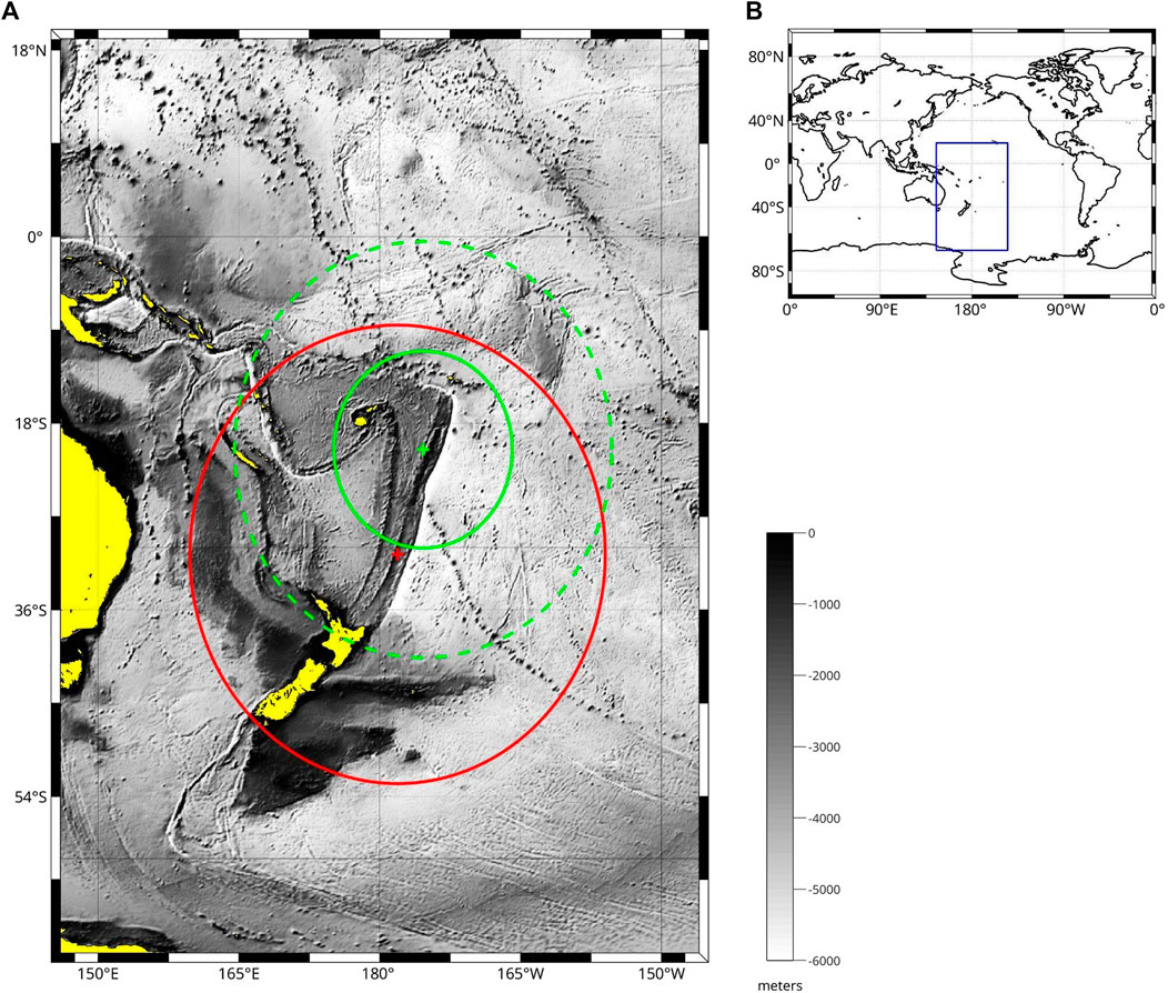
FIGURE 1. (A) The high resolution bathymetry map of the west Pacific ridge (grey levels), together with the HTHH volcano site and Kermadec Islands EQ epicentre (green and red cross, respectively), and the Dobrovolsky areas of the two analysed events (green and red circles; the dotted circle refers to HTHH energy released in air, with equivalent magnitude M = 7.1; Dobrovolsky et al., 1979); (B) the selected region in panel (A) with respect to the globe (blue box). Map produced by M_Map software (Pawlowicz, 2020).

Both the latter two geophysical events fostered a widespread interest and triggered studies due to their magnitude and impact on the entire globe (De Santis et al., 2022; D’Arcangelo et al., 2022 and the included references). Figure 1A also shows the circular Dobrovolsky areas relative to the magnitude of both events (see Eq. (1) in Section 2.1), delimited by a green circle for HTHH volcano eruption (equivalent magnitude for the energy released in the lithosphere), which is contained in the bigger one of Kermadec Islands EQ (red circle).

The discovery of the seismic/volcanic precursors was a goal of many studies and researches. The most important finding during the past two decades is that many of the earthquake precursors are electromagnetic rather than seismological, the reason for the numerous satellites developed in order to detect electro-magnetic emissions transmitted from earthquake regions, providing a huge amount of data, allowing us to overcome at once the criticisms of measurements from ground-level surveys (e.g., Campbell, 2003; Regi et al., 2021). Extensive coordination of numerous observations furnishes a mechanism of why and how the ionosphere is perturbed prior to an earthquake: the so-called Lithosphere-Atmosphere-Ionosphere Coupling (LAIC) models. Few hypotheses for the LAIC mechanisms are: i) electrostatic channel in which positive hole charge carriers in crustal rocks play the crucial role (Freund, 2011); ii) chemical channel in which radon emanating from the ground is the main player (Pulinets and Ouzounov, 2011); iii) atmospheric oscillation channel in which the perturbation in the pre-earthquake Earth surface excites the atmospheric oscillations travelling up to the ionosphere (Hayakawa et al., 2004; Molchanov and Hayakawa, 2008; Korepanov et al., 2009). All these mechanisms evidenced a clear sequence of the precursors and effects appearing from lithosphere to atmosphere and ionosphere.

Moreover, the model can be extended also to the magnetosphere, so introducing the concept of the Earth-atmosphere-ionosphere-magnetosphere (EAIM) system, a complex open dissipative nonlinear dynamical system (Chernogor and Rozumenko, 2008; Chernogor, 2011).

For obtaining a complete understanding of the preparation phase of the event, it is necessary to realise a multi-parametric and multi-layer study of the days before and after it; for this purpose, we need to consider different datasets, each one analysed with appropriate methods.

Regarding the seismic rate that precedes the volcanic eruption, Pesicek et al. (2018) identified seismic rate increases near volcanoes applying a common statistical tool, the β-statistic, to seismically monitor eruptions in Alaska of various style and determine the overall prevalence of seismic rate anomalies immediately preceding eruptions. Their results suggest that seismic rate increases are common prior to larger eruptions at long dormant, “closed-system” volcanoes, but uncommon preceding smaller eruptions at more frequently active, “open-system” volcanoes with more mafic magmas. HTHH eruption belongs to the former case study so we would expect some seismic rate increase before the eruption. This will be one of the issues addressed in the present seismic data analysis.

As regards the atmospheric analysis, Piscini et al. (2019) confirmed with a very high accuracy that atmospheric parameters, such as skin temperature (SKT), total column water vapour (TCWV), aerosol optical depth (AOD), sulphur dioxide (SO₂) show anomalies with a persistence of at least two consecutive days during the year that precedes eruptions with volcanic explosive index VEI4+.

In Liu et al. (2020), an analysis of climatological parameters in a long time period preceding the Ms 8.0, 21 May 2008 Wenchuan and Ms 7.0, 20 April 2013 Lushan EQs was carried out and put in evidence the all anomalous responses of four climatological parameters occurred within the 2 months before seismic events and indicated that the multi-parametric approach is beneficial to capture anomalous phenomena before strong EQs, highlighting the role of fluids in the preparation phase of large seismic events.

Shah et al., 2019 analysed some atmospheric parameters by statistical bounds of median and standard deviation for 2 months before and 1 month after the occurrence of three EQs of M_w>6.0 occurred in Pakistan and Iran during 2010–2017. They found abnormal atmospheric anomalies within 1 month before the main shock, suggesting that they are produced by a process that occurred at the ground-to-air interface due to the emanation of gases from the ground as a result of tectonic stress beneath the epicentral region.

As regards the ionospheric analysis, Total Electron Content (TEC) anomalies some days before and after seismic events were found by Adil et al. (2021) associated with an EQ of M 7.7 in Jamaica, and Kumar et al. (2021) concluded that the perturbations in TEC related to the major EQ of South West Banten, Indonesia, depend not only on the distance but also on the direction of the observation point from the epicentre, and finally Shah et al. (2020) attributed TEC anomalies, seen on the main shock day of M_w>6.0 EQ in Japan, to an anomalous electric field in the seismogenic zone triggered by stressed-rock. Adil et al. (2021) validated the ionospheric anomalies as possible seismic precursors analysing the atmospheric anomalies in relative humidity and Outgoing Longwave Radiation (OLR) to better explain their evolution from the lithosphere to the ionosphere through the atmosphere. Also TEC anomalies were analysed in a study by Li et al. (2016). In association with volcanic eruptions of VEI4+ in the interval time 2002–2015, they found that the occurrence rate of TEC anomalies depends on the characteristics of the eruption: they are higher before stratovolcano and caldera eruptions than that before shield and pyroclastic shield eruption. Moreover, they demonstrated that the TEC anomalies depend also on the latitudes of the volcano position: its occurrence rate has a descending trend from low to high latitudes. From this study, it results that the volcanic eruptions cause acoustic gravity waves that could lead to TEC perturbation. Moreover, Zhao et al. (2021) recently proposed a lithosphere-atmosphere-ionosphere model of ELF wave propagation radiated from seismic sources and the possibility to be observed by instrumentation on board of the CSES-01 satellite. Based on this model, two strong adjacent EQs (M_w 6.9 on July 7 and M_w 7.2 on 14 July 2019 in Indonesia) were analysed from electric field data in the ELF/VLF frequency bands recorded by space Electric Field Detector (EFD) on satellite CSES-01 (Zong et al., 2022). They found significant electric field anomalies (especially between 49 and 366 Hz) near the epicentre, mainly at night and along the ascending orbits, and that these abnormal enhancements seem to gradually diminish as the frequency increases.

In the present paper we deal with the comparison of the two significant geophysical events that occurred along the Tonga-Kermadec arc, i.e., the 2019 M7.2 Kermadec Islands EQ and the 2022 HTHH volcanic eruption. Two distinct observation single study analyses can be found in De Santis et al. (2022) and D’Arcangelo et al. (2022).

The first case study is the strong EQ that occurred on 15 June 2019, at 22:55:02 UTC (∼11:00 LT) of M 7.2 (as evaluated by GeoNet catalogue) with epicentre at Kermadec Islands at 30.644° S, 178.100° W, 46.0 km depth, about 600 km north-east of East Cape (https://earthquake.usgs.gov/earthquakes/eventpage/us6000417i/executive). The released energy generated a small tsunami that was recorded 17 min after the event at the nearby tide gauge of Raoul Island Boat Cove, New Zealand, with the run-up tsunami wave amplitude of 5 cm.

The second case study is the explosive eruption that occurred at the HTHH volcano (20.546° S, 175.39° W) on 15 January 2022, at 04:15 UTC (∼16:30 LT), with a plume reaching 30 km in the atmosphere and 600 km in diameter. Recent studies have shown several characteristics of this eruption, with particular phenomena occurring in the atmosphere and ionosphere. The Hunga Tonga explosion generated blast waves that present a cylindrical wave front and, depending on the trajectory, orientation and the state of atmospheric weather, the change of wave amplitude can reach two times for a constant distance from the volcano to the observatory (Chernogor and Shevelev, 2022). This volcanic event triggered atmospheric Lamb waves, recorded globally and observed from the geostationary satellite Himawari-8 (Otsuka, 2022). The Lamb waves also produced Travelling Ionospheric Disturbances (TIDs), recently observed at altitudes higher than 550 km from CubeSat GPS tracking data (Han et al., 2023). Medium-scale travelling ionospheric disturbances (MSTIDs) over the Central Mediterranean, with a horizontal wavelength of about 220 km and a period of about 35 min, were identified from the barometric–infrasonic stations installed on Italian territory by the Istituto Nazionale di Geofisica e Vulcanologia (INGV) and related to the tropospheric disturbances (Madonia et al., 2023). It was also discovered an ionospheric hole that occurred near Tonga at 05:00 UT, extended over a wide area of 160°-200° E and 25° S-20° N and lasted for about 11 h (Choi et al., 2023). This ionospheric hole merged with the equatorial ionisation anomaly (EIA) through depletion in the northern hemisphere.

For both cases in this paper, we introduced the particle precipitation study from the inner Van Allen Belts, the so-called Electron Bursts (EBs), as detected from some satellites. For the first time, EBs were analysed at the time of an explosive eruption and in connection with other ionospheric observations related to seismicity. In fact, sudden increases of electron fluxes near the South Atlantic Anomaly (SAA) were already discovered from the MARIA experiment on board the SALYUT-7 orbital station, occurring in relation with strong seismic activity (Voronov et al., 1989). Moreover, the association between electron losses and strong EQs was investigated by means of the McIlwain or L-shell parameter in the range of the inner belts from 1.1 to 1.4 (Aleksandrin et al., 2003; Sgrigna et al., 2005). Data belonging to the NOAA’s Polar Orbiting Environmental Satellites (NOAA-POES) confirmed a statistical correlation between high energy precipitating electrons and West Pacific strong EQs always for low L-shell electrons (Battiston and Fidani, 2010; Battiston and Vitale, 2013; Fidani, 2015; Fidani, 2018; Fidani, 2020; Fidani, 2021; Fidani, 2022). For both case studies analysed—Kermadec Islands EQ and HTHH eruption—the corresponding L-shell parameter estimated through Shepherd (2014) algorithm is L∼1.1, which falls within the above mentioned range.

In this work, our principal motivation is to understand the physical processes that took place in this tectonic-volcanic zone considering these two important events, focusing our attention on the similarities and differences among them. We start to expose the methods and data used in each layer analysed. Then, we show the results found in lithosphere, atmosphere and ionosphere to finally reason on the processes assumed to explain the observed phenomena. Most of the presented results are based on the previous publications about single case studies (De Santis et al., 2022; D’Arcangelo et al., 2022), here also including some new analysis to present a more complete study of this complex area and to identify the most important similarities and differences.

2 Data

Despite the different nature of the events analysed, very few differences are evidenced for the characteristic parameters taken into account in the study: the volcanic eruption released an energy in lithosphere associable to an EQ for lithospheric analysis; also a recent study confirmed the great seismic activity leading to the main eruption (Thurin et al., 2022). The parameters on the atmosphere and the ionosphere possibly influenced by seismic and volcanic events are similar so they were investigated in detail.

2.1 Lithospheric data

The Kermadec-Tonga subduction zone is one of the most active regions of the Earth due to the high velocity of subduction of the Pacific plate beneath the Australian plate. Since the Gutenberg-Richter law (Gutenberg and Richter, 1954) demonstrated that the b-value parameter depends on the source environment of the region, a seismological study needs to examine its value. So, in order to study the seismicity of the great geophysical events, we focused our attention on this parameter and, consequently, on the magnitude of completeness (Mc) to determine the tectonic regime of the area. Finally, it was possible to evaluate the Revised Accelerated Moment Release (R-AMR, introduced by De Santis et al., 2015). The maximum distance where the precursory effects of an EQ could be detected is defined by the Dobrovolsky strain radius ρ, depending on the magnitude M (Dobrovolsky et al., 1979):

$\rho ={10}^{0.43M}\left(km\right)(1)$

For both events, the USGS catalogue was used, which contains data from a worldwide network of seismic stations. Moreover, for analysing in detail the Kermadec Islands EQ, also the GeoNet catalogue—national New Zealand—was considered, since it admits lower Mc (even lower than 2.0). The time intervals considered for the events are between 01 January 2018 and 14 June 2019 for Kermadec EQ and between 01 January 2021 and 16 January 2022 for HTHH eruption.

2.2 Atmospheric data

There are many atmospheric parameters that can be influenced by terrestrial geophysical events like EQs and eruptions (e.g., Piscini et al., 2017; 2019). For identifying the correlated signals, we need to compare their behaviour at the time near the event with the historical background: in both case studies about 40 years of past data were considered. The data used for this purpose come from the European Centre for Medium-range Weather Forecasts (ECMWF) datasets; moreover, for seismic events the data were taken also from NASA-NOAA (National Oceanic and Atmospheric Administration). For both events, it was considered the ERA-5 model for its higher temporal (1 hour) and spatial (0.25°×0.25°) resolution composed of 137 levels from surface to 80 km height, updated to present, in quasi-real time. Concerning Kermadec Islands earthquake, we focused on the ECMWF Copernicus Atmosphere Monitoring Service (CAMS) climatological dataset and on the Modern-Era Retrospective analysis for Research and Applications—version 2 (MERRA-2): it represents a long-term global reanalysis to assimilate space-based observations of aerosols from 1980 to present, updates once per month, with the spatial resolution of 0.625° longitude and 0.5° latitude overlapping the area of interest and the same hourly temporal resolution.

2.3 Ionospheric and magnetic data

Ionosphere was investigated taking into account observations in-situ at ground and by satellites, by ionosondes and Global Navigation Satellite System (GNSS) receivers, respectively. According to the LAIC models (Freund, 2011; Pulinets and Ouzounov, 2011), there are various operating satellites whose instruments may be able to detect ionospheric effects eventually leading to an imminent EQ. Nowadays, it is possible to count on the availability of the European Space Agency (ESA) Swarm constellation of three identical satellites in a quasi-polar orbit (Alpha and Charlie at around 460 km altitude and Bravo at 510 km), and of the first China Seismo-Electromagnetic Satellite (CSES-01) which flies in a sun-synchronous orbit at around 500 km of altitude. In this work for both events, we took into account both Swarm magnetic vector data (MAGX_LR_1B, with a low rate of 1 Hz) and magnetic vector data (MAGX_HR_1B, with a high rate of 50 Hz). Electron density datasets provided by the Langmuir Probe (LAP) of the Electric Field Instrument (EFI) at 2 Hz were also considered (available at ESA Swarm FTP and HTTP Server, https://www.swarm-diss.eo.esa.int). Various payloads provide data that are routinely delivered by CSES-01 satellite and used in the present work: the Langmuir Probe (LP) provides plasma measurements as electron density and temperature (1 s and 3 s in burst and survey modes, respectively); the High Precision Magnetometer (HPM) and the Search Coil Magnetometer (SCM, for further technical details refer to Cao et al., 2018) provides accurate geomagnetic field measurements at low and high frequency, respectively; the Electric Field Detector (EFD, for further technical details refer to Diego et al., 2021) furnishes precise electric field data (www.leos.ac.cn). For analysing the possible abnormal electromagnetic emissions associated with seismic activities, different frequency bands of the load recorded by EFD were inspected: DC-ULF (0–16 Hz); ULF-ELF (6–2.2 kHz); ELF-VLF (1.8–20 kHz).

As regards ground observations, we use GNSS data from the GeoNet GNSS/GPS network (https://www.geonet.org.nz/) looking for anomalies in the vertical TEC (vTEC) during the preparation phase of both the events. In our previous study on the HTHH eruption (D’Arcangelo et al., 2022), also vTEC maps produced by the International GNSS Service (IGS) (https://cddis.nasa.gov/) were analysed, focusing on the nearest grid point location with respect to the volcano during the day of the eruption, compared to the days before and after it. Ionosonde data during the eruption day from the global ionosonde network, providing the limit-transmitting frequency of the F2 layer, the so-called foF2 parameter—not available for Kermadec EQ—were also used in the study.

Electron fluxes with energy ranging from 40 keV to 2.5 MeV were collected by NOAA and MetOp polar orbiting satellites. Instruments on-board such satellites continuously monitor particle fluxes at ionospheric altitudes which include the radiation belt population (Davis, 2007). The data from Meteorological Operational satellite program of Europe (MetOp) and NOAA-POES were used for the analysis of both events. The first one consists of three satellites, MetOp 1, 2 and 3, launched in 2006, 2012 and 2018, respectively, are in the range 810–830 km of altitude; a program born within a collaboration between ESA and the European Organisation for the Exploitation of Meteorological Satellites (EUMETSAT). Each NOAA satellite operates at the particular range of 800–890 km in altitude. The satellites considered in this study are NOAA-15, -18 and −19, and MetOP 1, 2 and 3 (data available at https://www.ngdc.noaa.gov/stp/satellite/poes/dataaccess.html). The inclination angles of these polar satellites are between 98.5° and 98.8°, and their periods are between 101 and 103 min. During the analysed time intervals, their equatorial crossing local times are 06:57 LT for the NOAA-15, 08:40 LT for the NOAA-18, and 04:56 LT for the NOAA-19 all along descendent orbits, whereas MetOp equatorial crossing time is 09:05 LT for MetOp 1, and is around 09:30 LT for MetOp 2 and 3. However, MetOp 2 was retired in 2021, so there was no data in 2022 at the time of HTHH eruption. For the Kermadec Islands EQ, data from all 6 satellites were analysed, while data from only 5 satellites were analysed at the time of the recent volcanic eruption. The particle detectors working on-board all these satellites are identical and composed of eight solid-state telescopes called Medium Energy Proton and Electron Detectors (MEPED). They consist of two proton-telescopes, monitoring the flux in five energy bands in the range 40 keV to 2.5 MeV, two electron-telescopes in three energy bands in the range 40 keV to 2.5 MeV, and four omnidirectional detectors sensitive to proton energies above 16 MeV. As past works found positive correlations between electron burst and strong EQs, only electron fluxes were used in this work after being corrected for proton contamination. The archive record of electrons and protons was provided starting from 2012 (from the link https://www.ncei.noaa.gov/data/poes-metop-space-environment-monitor/access/l1b/v01r00/) in the netCDF (network Common Data Form) format, with averages on all the data every 2 s.

3 Data analyses and results

3.1 Seismological data analysis

The analysis starts with the seismological data taken by GeoNet for the Kermadec EQ: the analysed catalogue comprised all earthquakes from 1 January 2018 until the last event before the mainshock; inside the Dobrovolsky area 18,291 events were identified. From these, we calculated the magnitude of completeness (Mc) as a time function sliding the time window containing 150 EQs by steps of 5 events. Mc values furnished by GeoNet are between 1.8 and 2.2 for the period considered (De Santis et al., 2022). Also the energy released by the main eruption of HTHH could be associated with a seismic event of M 5.8–6.0. Considering this last value of magnitude and the corresponding Dobrovolsky area we obtained 388 events and a Mc = 4.3, using the USGS catalogue. The Mc allows us to filter the catalogue in order to calculate the b-value parameter. This parameter is important in a seismic study since it depends on the physical and tectonic conditions: lower values are associated with a possible origin of an imminent seismic event, indicating asperity area (Scholz, 2015; Nanjo and Yoshida, 2021).

At this point, applying the Accelerated Moment Release (AMR) method in its Revised version (De Santis et al., 2015; Cianchini et al., 2020) to the catalogue it is possible to see the accelerating seismicity, typical in the preparation process of many mainshocks. AMR is based on the sum of the Benioff strain (i.e., the cumulative Benioff strain) as estimated for each i-th foreshock with the formula: s_i= $\sqrt{E_i}$, with $E_i$ = ${10}^{1.5*M+4.8}$ (e.g., Cianchini et al., 2020). R-AMR with respect to AMR weights the Benioff strain of foreshocks by the reciprocal of their distance to the mainshock epicentre in an area usually larger than the fault size but smaller than the Dobrovolsky region. This quantity is also called reduced Benioff strain (Cianchini et al., 2020). The acceleration is confirmed by the low values of C-factor, defined as the ratio between the root mean square (rms) of the residuals of the non-linear (power-law) and the one of the linear fit (Bowman et al., 1998) of the reduced Benioff strain:

$C=\frac{{rms}_{nlin}}{{rms}_{lin}}(2)$

It gives the quality of the seismic acceleration with respect to a linear trend (typical cumulative strain of a random background seismicity), in particular the lower the C-factor (i.e., closer to zero), the higher the acceleration. This can be physically explained by the fact that a normal random seismicity without acceleration shows a linear cumulative Benioff strain, while an acceleration before a large earthquake usually deviates from the linearity with a power law.

As shown in R-AMR analysis in Figure 2 (y-axis is the reduced Benioff strain, while x-axis is time), we evidenced important parameters obtained: R₀ represents the distance in km from the fault of concern where the EQ occurred while R₁ indicates the distance in km of the i-th EQs from the centre of the chosen area; t_f(pred) the time of the imminent predicted event; R_adj² is the coefficient of determination, a measure of the quality of the fit; and finally the predicted magnitudes, M(A) and M(B), two values which limit the interval of magnitude that we expect from these conditions. It is evident, from values of C-factor lower than the unit, the accelerating seismicity for both events. The seismicity is, in general, higher for the Kermadec Islands EQ, as shown in its distribution at the lower panel of Figure 2, and also its acceleration (C≈0.6 compared with C≈0.7 for HTHH) is higher for this event, as expected taking into account the seismic character of the Kermadec event. Another important result that we obtained from this study is the accuracy of the expected magnitudes for imminent events: M 7.1–7.4 for Kermadec Islands EQ and M 6.4–6.7 for HTHH eruption. An interesting similarity between the two cases is that the percentage of earthquakes in the inner region, i.e., that delimited by R₀ and indicated with red circles in Figure 2, is almost the same, i.e., a little less than 1%. However, the major differences are their absolute number and their occurrence: in the Kermadec Islands EQ, these inner earthquakes are 12 and appear intermittently at each seismic crisis, while in the HTHH eruption, there is just one inner earthquake and appears just before the great eruption. Finally, the time predicted from this study for the Kermadec Islands event is 07 July 2019 (i.e., ∆T, the difference between time predicted and time of the event, about 22 days after the main shock) while for the HTHH eruption is 23 March 2022 (i.e., about 67 days after the eruption), demonstrating again the higher accuracy of the method for seismic event prediction with respect to volcanic eruption.

FIGURE 2

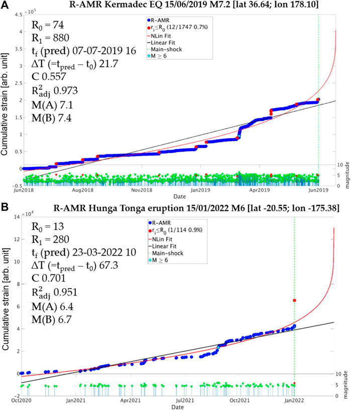
FIGURE 2. The R-AMR analysis of (A) the New Zealand catalogue referred to M7.2 Kermadec Islands EQ; (B) HTHH main eruption of 2022. In both cases, y-axis represents the reduced Benioff strain, while the x-axis represents the time. It is evident the increased seismicity for the algorithm applied. See text for descriptions of the parameters included into the two plots.

3.2 Atmospheric data analysis

LAIC models evidence that tectonic events, like EQs and volcano eruptions, could release trace gases and alter atmospheric parameters such as temperature, humidity, outgoing longwave radiation (OLR) even before their occurrence (Pulinets and Ouzounov, 2011). For analysing the atmospheric parameters influenced by the events under study, we consider the ECMWF Reanalysis v5 (ERA5) for both events and Copernicus Atmosphere Monitoring Service (CAMS) for Kermadec EQ, climatological datasets were analysed applying a Climatological Analysis for Seismic Precursor Identification (CAPRI) algorithm (see for details Piscini et al., 2017; 2019) with a spatial grid of 0.25°×0.25°. This analysis consists of comparing the parameters in the three-four months preceding the event with the same seasonal period of the historical time series of the previous around 40-years (1979–2018 for Kermadec Islands EQ and 1980–2021 for HTHH eruption). An anomaly is detected when the trend of the year of the geophysical event overpasses positively the mean of the historical time series by twice the standard deviation (σ). The spatial distribution has been investigated in an area of 10°×10° in latitude and longitude around the Kermadec EQ epicentre and 1°×1° around the HTHH volcano. The spatial distribution (respective maps are shown in De Santis et al., 2022; D’Arcangelo et al., 2022) allows to corroborate the position of maximum value with respect to the event source. Also the data of a year without significant events were taken into account for the confutation analysis (in our case 2018 and 2021).

In particular, for the seismic event we focused our attention on data of AOD, SKT, outgoing longwave radiation (OLR), total column water vapour, methane (CH₄) and SO₂. The analyses of these latter three are shown in Supplementary Figure S1 (Supplementary Material) in comparison to those referred to the volcanic eruption. They show minor anomalies not comparable to those of volcanic events and the persistent anomalies present the maximum value not centred on the epicentre. Actually we also analysed other physical quantities such as cloud cover, the relative humidity, the ozone, the carbon monoxide and sulphur sulphate, but no statistical anomaly was found with respect to the historical background, so we did not show here any of their results. For the HTHH eruption, in addition to SKT and OLR, we also considered data of temperature at 2 m (2 mT), cloud cover and ozone content. The parameter that showed more anomalies before the EQ is AOD: a 6-day persistent anomaly starting 104 days before the event (3 March 2019) and two single anomalies 59 and 16 days before (April 17 and 30 May 2019, respectively, Figure 3B). The SKT also shows two single anomalies: one 94 days before (13 March 2019) and another again 16 days before (30 May 2019). In the same months, we saw three single anomalies of TCWV: 93, 76 and 16 days before the event (on March 14 and 31, and 30 May 2019, respectively). The OLR parameter exhibits a 3-day persistence anomaly started 37 days before the event (9 May 2019) and two single anomalies 31 and 16 days before (May 15 and 30). Whereas, the HTHH eruption generated various persistent anomalies in the OLR (Figure 3F): one 4-day persistent starts 82 days before (25 October 2021), two 2-day persistent from 76 to 59 days before (October 31 and 17 November 2021, respectively) and two single anomalies 47 and 13 days before (29 November 2021 and 2 January 2022, respectively). The temperature parameters, 2 mT and SKT, present a single anomaly 50 and 49 days before (November 26 and 27, 2021). In addition, a single anomaly of cloud cover was found 67 days before (9 November 2021).

FIGURE 3

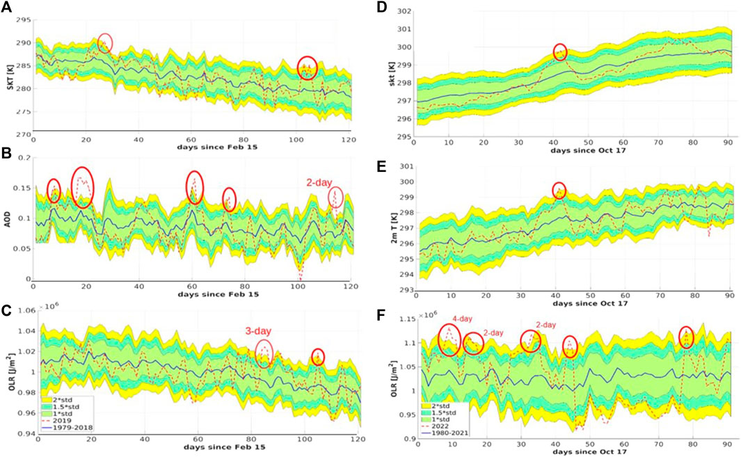
FIGURE 3. ECMWF climatological catalogue analysed for Kermadec Islands EQ (A–C) referred to 4 months before the mainshock) and for HTHH main eruption (D–F) referred to 3 months before the eruption). The multiples of standard deviation (σ) from the mean of the historical time series are indicated with different colours: 1.0σ green; 1.5σ cyan; 2.0σ yellow. The red circles put in evidence the anomalies identified by the algorithm CAPRI applied with the respective persistence, if more than 1 day. (A), (D) SKT (Skin Temperature); (B) AOD (Aerosol Optical Depth); (E) 2 mT (temperature measured at 2 m of altitude); (C, F) OLR (Outgoing Longwave Radiation).

3.3 Ionospheric data analysis

With the aim of finding possible anomalous signals in the ionosphere, we considered magnetic and electric fields together with electron density data from low earth orbit (LEO) Swarm satellites and CSES-01, and TEC from ground GNSS stations. Electron Bursts (EBs) were also analysed from NOAA and MetOp satellites.

The geomagnetic activity preceding and during the two events shown in S1 of Supplementary Material in the form of the time evolution of two indices, Dst and ap, is accounted for supporting the discussion of the extracted ionospheric anomalies, potentially related to their preparation phase. Both events were preceded by weak and moderate geomagnetic disturbances in the few days before the events. During the last hours on June 8 and 13, 2019 (i.e. 7 and 2 days before the EQ), moderate and weak increases of the ap index were observed, respectively (Supplementary Figure S2B). The first one was associated with sudden variations of horizontal magnetic field at low latitudes, indicated by the Dst index trend (Supplementary Figure S2A). During the last hours on January 8 and 14, 2022 (i.e. 7 and 1 days before the eruption), moderate increases of the ap index were also observed (Supplementary Figure S2D). The sudden variations of horizontal magnetic field at low latitudes on January 14 (Supplementary Figure S2C) were more intense and had repercussions on the ionosphere for a few days.

3.3.1 Total electron content (TEC) data analysis

This analysis offers, for Kermadec EQ, three possible anomalies individuated using a two-station approach, the most promising among different methods proposed (De Santis et al., 2022). With this approach we define the relative difference ∆TEC as:

$∆\text{TEC}\left(\mathrm{t}\right)=\left[\text{TEC}\left(\text{station\hspace{0.17em}}1,\mathrm{t}\right)-\text{TEC}\left(\text{station\hspace{0.17em}}2,\mathrm{t}\right)\right]/\text{TEC}\left(\text{station\hspace{0.17em}}2,\mathrm{t}\right)(3)$

where station 1 and station 2 are closer and farther GNSS stations to the EQ epicentre (or below, to the eruption location), respectively. TEC values are actually vertical TEC calculated every 30 s and calibrated applying the techniques described in Ciraolo et al. (2007) and Cesaroni et al. (2015) to RINEX data. We defined an anomaly when ∆TEC overcomes the value of the linear trend over the 4 months prior to the EQ by 2 TECU for at least 5 min. As reported in De Santis et al. (2022), the first anomaly was seen 89 days before the event (18 March 2019); the second was found 29 days before (17 May 2019); the third occurred 10 days before (5 June 2019).

Regarding the HTHH eruption, we applied the same approach but identifying the anomalies when the ∆TEC overcomes the linear trend by 4 TECU. The data from the same GNSS stations of the GeoNet GNSS/GPS network already considered for Kermadec Islands EQ are used, with distances from the eruption location of about 1,000 km and 3,280 km for the closer and farther stations, respectively. The results are shown in Figure 4, with the only anomaly found under magnetically quiet conditions occurring on 31 December 2021, i.e. 15 days before the eruption.

FIGURE 4

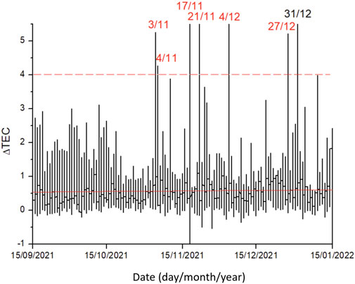
FIGURE 4. TEC anomalies found before HTHH eruption considering the same GNSS stations already used for Kermadec Islands EQ. All red anomalies are found during disturbed geomagnetic periods (Kp>2 or |Dst|>20 nT). Only the anomaly on 31 December 2021 (i.e. 15 days before the eruption) occurred during quiet magnetic times.

3.3.2 Satellite magnetic and electron density data analysis

We analysed the Swarm and CSES-01 satellite magnetic data following the MASS (MAgnetic Swarm anomaly detection by Spline analysis) method. This method uses the first differences divided by the time interval from a sample and the next one and b-splines to remove the long trend (details about the method in De Santis et al., 2019). For the Kermadec Islands EQ, we considered 150 days before the main shock: only 110 days before (25 February 2019) a promising anomaly was found in quiet geomagnetic conditions (daily average values ap=1.3 nT; Dst=3.2 nT) seen by Swarm and CSES-01 satellites, within the Dobrovolsky area, as shown in Figure 5. The anomalous signal is more evident in the Y-component of the geomagnetic field, as expected for anomalies of internal origin, especially for longer time scales (Pinheiro et al., 2011).

FIGURE 5

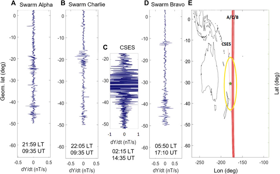
FIGURE 5. First derivative of the Y-component of magnetic field analysed by Swarm satellites (Alpha, Charlie, Bravo represented at (A, B, D), respectively) and CSES-01 (C) on 110 days before the seismic event (25 February 2019), the corresponding local and universal times of the intermediate position of the satellite are indicated in bold. The average daily geomagnetic activity indices are ap = 1.3 nT and Dst=3.2 nT, which classify the day as magnetically quiet. In panel (E) the geographic map is represented with the satellite tracks in red and the Dobrovolsky area, around the star of the epicentre, in yellow.

For the volcanic eruption, the satellite tracks inside the Dobrovolsky’s area and also over the conjugate magnetic point of the volcano have been considered. Unfortunately, the geomagnetic storm of a few preceding days to the eruption could cover the possible signals. However, on the eruption day the comparison of the first differences of the total intensity F of Swarm satellites shows a peculiar characteristic: a magnetic perturbation is individuated on the east-tracks to the volcano but it disappears on the west-track of Bravo satellite (Figure 6). To better understand this characteristic, it was plotted the magnetic field direction based on the 13th generation of the International Geomagnetic Reference Field model (IGRF-13, Alken et al., 2021) at sea level in black and also extracted from direct measurements of absolute scalar magnetometer (ASM) of the Swarm Bravo at its altitude in orange. Since the arrows of the perturbation point to east, probably the perturbation follows the field direction.

FIGURE 6

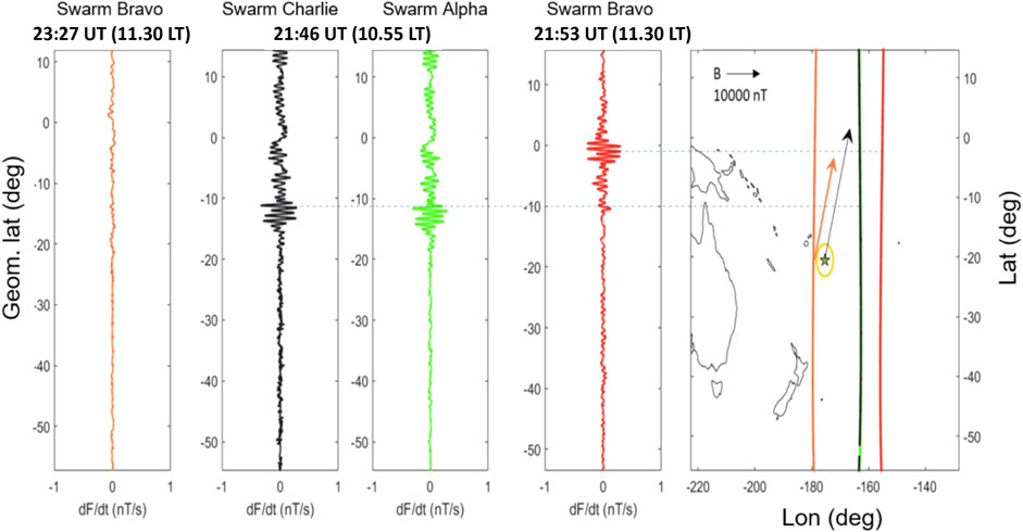
FIGURE 6. Comparison of the first differences of the total intensity F of the Swarm satellites of the eruption day (i.e. 15 January 2022), the corresponding local and universal times are indicated at the top: the values of the geomagnetic indices are Dst=−35 nT and ap=39 nT, so there were some geomagnetic disturbances. On the right, the geographic map shows the satellite tracks with respect to the Dobrovolsky area, in yellow, and the volcano position, represented with a star. The arrows indicate the horizontal directions of the geomagnetic field measured by the ASM of Swarm Bravo satellite in orange and in black at sea level, based on the IGRF-13 model (Alken et al., 2021). While F comes from the scalar magnetometers of Alpha and Bravo, that of Charlie has been calculated from the magnetic field components measured by the fluxgates, since the scalar magnetometer on board of Charlie satellite operated for only a few months after the beginning of the Swarm mission.

Also the electron density (Ne) shows interesting characteristics before both events. In Kermadec Islands EQ case, the Swarm Alpha satellite acquired, in very quiet geomagnetic conditions, an anomalous Ne track 119 days before (16 February 2019) at 28° S (for more details about this anomaly and Ne analysis consult De Santis et al., 2022). For the HTHH eruption instead, the main important result on Ne analysis was given by the Langmuir probe (LAP) data of CSES-01. The track relative to the eruption day shows two disturbances: the first one, at the volcanic explosion, possibly produced by an electromagnetic wave, and the second one may coincide with the arrival of acoustic-gravity wave signal to the F2 ionospheric layer (considering the relative velocity of this type of wave).

We investigated the magnetic field fluctuations at Swarm’s altitudes during the EQ day (15 June 2019) following the same methodology of D’Arcangelo et al., 2022 for the HTHH eruption. In particular, we performed a spectral analysis of the magnetic signals provided by the vector magnetometer and stored in the north–east–center (NEC) reference frame at 1 Hz sampling rate, here indicated as B_N, B_E and B_C components, respectively. Before performing the spectral analysis, the magnetic data were differentiated in order to: (a) reduce the typical red-noise trend of the spectra in the ionosphere (e.g., Francia et al., 2013) for magnetospheric applications); (b) mitigate the effect of satellite’s low polar orbits which determines an apparent high variation of the main magnetic field in each time window as trends or offsets, due to standard latitudinal dependence of geomagnetic field.

For the investigations, we computed the dynamic Power Spectral Density (PSD) of each magnetic field components: we considered a 400 s moving time window with a step size of 13 s spanning the whole time series; for each sub-interval we computed the PSD through a fast Fourier transform (FFT) algorithm applied to magnetic field measurements and by using the Hamming taper. Each spectrum was smoothed over 3 adjacent frequency bands by using a triangular window (final frequency resolution ∼5 mHz) increasing the reliability of the resulting spectra without losing in frequency resolution (e.g., Regi et al., 2013; 2014a; b). The final spectra were not converted by means of the transfer function of the difference in order to make more clear ultra-low frequency (ULF, 1 mHz–5 Hz) signals. In addition, we computed the distance “d” of each satellite position projected on ground with respect to the epicentre position and assuming the ground as a spherical surface.

We first investigated the time interval strictly near to the Kermadec Islands main shock. Figures 7A, D show, for Swarm A and B, the (2 times) differentiated magnetic field during 21:30–24:00 UTC on 15 June 2019 (under quiet geomagnetic conditions; Supplementary Figure S2A, B), the satellite’s latitudes and their distances “d” with respect to the epicentre (Figures 7B, E), and the total PSDs, i.e., the sum of the PSDs of each magnetic field component (Figures 7C, F). The second order difference was applied only to time series for making more clear the magnetic fluctuations, while the PSDs are computed on first order differenced time series as in D’Arcangelo et al. (2022). The high fluctuation and power levels observed correspond to the high latitude sectors of the Swarm satellite’s orbit (|lat| > 55°–60°) and are due to the well-known high latitude geomagnetic activity. The dynamic spectra clearly show the occurrence of ULF fluctuations approximately in the ∼1–150 mHz frequency range, while at higher frequencies no significant signals emerge. Interestingly, the PSD also seems to be symmetric around the geographic equator and in the Kermadec sector, which is crossed approximately at 22:05 by Swarm A and at 21:52 UT by Swarm B and at 23:40 UT only by Swarm A (lat=0 is indicated by horizontal dashed lines in panels B and E). The observed broadband activity without a symmetry for Swarm B around 23:25 UT is probably attributable to the large value of d (∼11,000 km) with respect to that observed for Swarm A (d∼3,100 km). Regarding the first time interval the higher ULF activity (higher PSD values) is more intense at Swarm A altitude, which is lower than the altitude of Swarm B. These results are in agreement with that found in previous investigations (D’Arcangelo et al., 2022) for HTHH eruption.

FIGURE 7

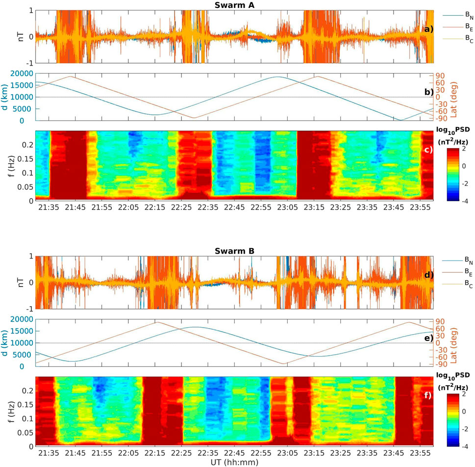
FIGURE 7. Differentiated magnetic data from Swarm A and B (A, D) during 15 June 2019, together with the satellite-volcano distance “d” and geographic latitude (B, E) and sum of the dynamic PSD of all components, here indicated with S (C, F). The large high power intervals at high latitudes (|lat| > 55°–60°) are due to high latitude phenomena.

Is a matter of fact that the part of the examined frequency range may be affected by well-known geomagnetic pulsation Pc3 (10–100 mHz) due to the transmission of upstream waves generated by solar wind-magnetosphere interaction (e.g., Regi et al., 2014b). In a separated analysis we computed the expected frequencies of upstream waves through the empirical relationship f_uw≃6B (mHz) (Troitskaya and Bolshakova, 1988), where B is the IMF strength measured in nT. By using satellite measurements of solar wind and interplanetary magnetic field conditions at 1 AU provided by OMNIWeb (https://cdaweb.gsfc.nasa.gov/), we found that the 95% of upstream wave frequencies are expected in the range ∼15–30 mHz. Therefore, the frequency range of eventually transmitted upstream waves regards the very restricted part of the entire frequency range here investigated. In addition, the observed ground occurrences of upstream waves at mid-low latitudes is expected in the morning hours (e.g., De Lauretis et al., 2010), contrary to the observed time independent ULF signals at Swarm satellites altitudes. By a visual inspection we compared the time series of predicted Pc3 frequency with PSD at both satellites, Swarm A and B, and we did not find any correspondence.

The investigations were extended to the whole day of 15 June 2019, by restricting the analysis to time intervals for which d<7000 km and |lat|<60° (i.e., excluding the polar regions); for these time intervals we computed the ULF power track by integrating the total PSD in the 1–150 mHz frequency range. Figure 8 shows ULF waves power tracks for both Swarm satellites.

FIGURE 8

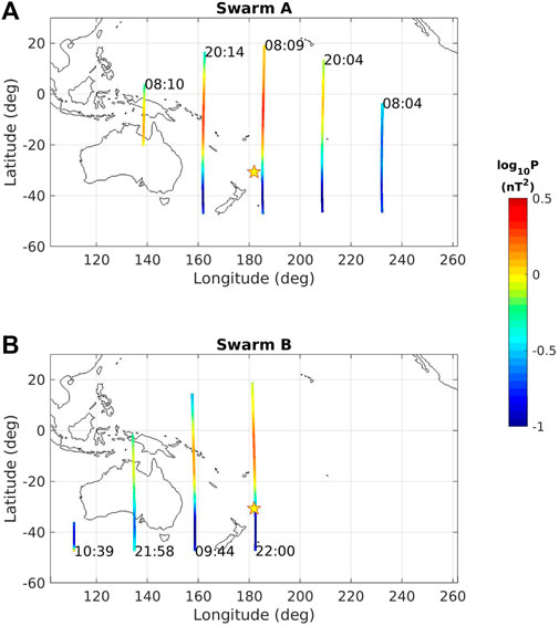
FIGURE 8. Power tracks in the 1–150 mHz ULF range at Swarm A (A) and B (B) during 15 June 2019. The local times of the track beginning are indicated. The Kermadec Islands’ position is marked by a star.

It can be seen that higher average power levels are attained at Swarm A altitude, accordingly with that found in Figure 7. Moreover, the power track levels seem to be independent of local time, suggesting that our observations are probably related to a large area located northward the Kermadec Islands (indicated by a star). Based on these results we retain that probably the observed ULF signals came from the examined regions below the satellites.

3.3.3 CSES-01 electric and magnetic field spectral analysis

For the Kermadec event we analysed SCM and EFD datasets of CSES-01 from May 1 till 30 June 2019, i.e., from 1 month and half before the mainshock to 15 days after. Data management of CSES-01 satellite releases EFD spectra in different frequency bands specified as follows, slightly different from the standard classification: Extra Low Frequency (ELF, 6–2200 Hz), Ultra Low Frequency (ULF, DC-16Hz), Very Low Frequency (VLF, 1.8kHz–20 kHz) and High Frequency (HF, 18kHz-3.5 MHz). We plotted and visually inspected all spectrograms related to the satellite orbits crossing the Dobrovolsky area with the aim of finding peculiar features. We performed dynamic spectra of the magnetic field data and found no peculiar feature which could be related to the preparation phase or occurrence of the EQ at Kermadec Islands. We detected an ULF signal which often emerges in the Dobrovolsky area, as well as in other areas in the same latitude range. In Supplementary Figure S3 of Supplementary Material we show as an example of this kind of signal, emerging just before (about 8 h, during local nighttime, in ascending orbit) and after (about 2 h, during local day time, in descendent orbit) the occurrence of the EQ at Kermadec Island. The Dst value shows that in both cases the magnetospheric conditions are quiet, being −4 nT and −10 nT, respectively. We notice a sparse presence of energy content, enhanced in the Dobrovolsky’s area after the EQ. It emerges on all (i.e., X, Y, Z) components, with greater evidence on the Y-East component, which is less contaminated by external field variations.

Regarding the electric field, we analysed the dynamic spectra in the ELF, ULF, VLF and HF frequency bands. A noteworthy feature emerges in the VLF range, in particular a power enhancement at about 20 kHz within the Dobrovolsky area (a sample is shown in Figure 9). This feature is persistent, regardless of the magnetic activity level, both before and after the EQ, inside the Dobrovolsky area crossed during local nighttime.

FIGURE 9

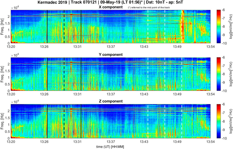
FIGURE 9. Dynamic spectra of the electric field from CSES-01 on 9 May 2019 (orbit number 70121, during local nighttime, in ascending orbit) in the frequency range DC-25 kHz. The solid black lines indicate the limits of the Dobrovolsky area; the black dashed line corresponds to the time of the minimum distance between the epicentre and the orbit; white dashed lines indicate the region with magnetically conjugate latitude with respect to the Dobrovolsky area. This is an example of the power enhancement at about 20 KHz within the Dobrovolsky area.

We analysed electric field power spectra also for the HTHH volcanic eruption from 1 December 2021 until 15 January 2022 (then, until January 29, EFD data are missing). We could not analyse SCM data which are available only until 31 December 2021. In Figure 10 a dynamic spectra of the electric field in the frequency range DC-25 kHz for 15 January 2022, the very day of the main eruption (10 h after the eruption) is shown. Within the Dobrovolsky area there is a “smiley-like” signal which resembles a VLF saucer (Parrot et al., 2011; Moser et al., 2021). We remark that this feature in the Dobrovolsky’s area is peculiar of this particular day and does not emerge on any other day in the whole analysed period.

FIGURE 10

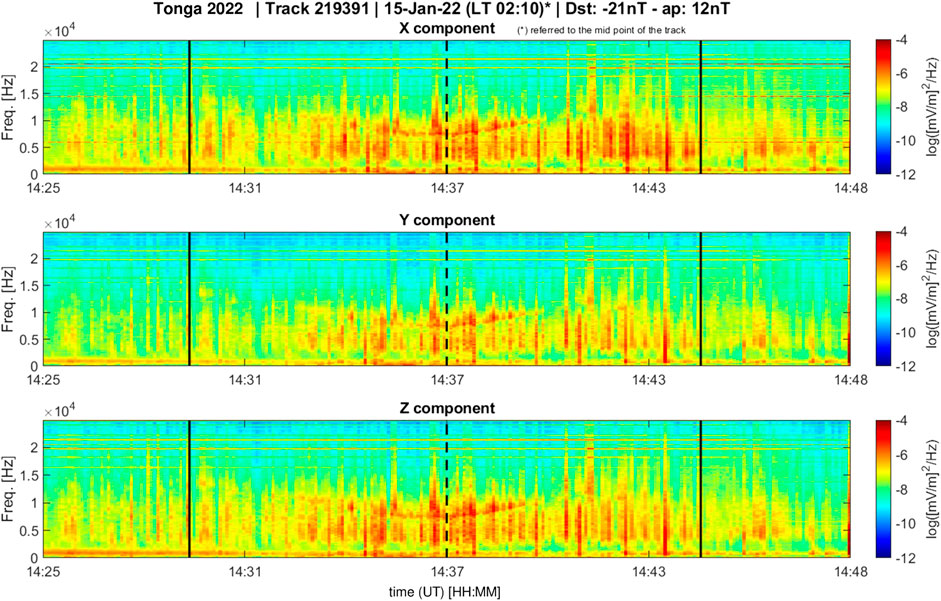
FIGURE 10. Dynamic spectra of the electric field from CSES-01 on 15 January 2022 (orbit number 219391) in the frequency range DC-25 kHz. The solid black vertical lines indicate the limits of the Dobrovolsky area; the dashed line corresponds to the time of the minimum distance between the epicentre and the orbit.

Some days before the event, the dynamic spectra of the electric field in the ULF band show, within the Dobrovolsky area, a signal that resembles a “pinnacle”, i.e., an increase in power for a limited time in the entire frequency band (f<20 Hz), with decreasing power for increasing frequency. In particular, this feature is evident on December 11 (i.e. 35 days before the eruption, Figure 11A), 16 (i.e. 30 days before) and 21 (i.e. 25 days before), 2021 around 14:40 UT, corresponding to local nighttime. This feature also persists in most of the days between 11 and 21 December, as well as in the preceding and following days, but in those 3 days it is particularly evident. On 21 December 2021 the “pinnacle”-like signal (not shown here) is immersed in a much greater generic signal, probably due to the fact that the eruptive activity began the day before. We also remark that the three major events are separated by 5 days, equal to the revisiting period of the satellite orbit. So the signals were emitted in all three cases from the same region. In the other frequency bands, no corresponding signal is observed, so we can exclude that it can be the signature of a lightning strike. These “pinnacle” signals are shortly followed by a broadband signal at about 10 Hz; a similar energy gathering can be seen also at the highest frequencies of the HF band, at about 2 MHz (Figure 11B). We notice that, contrary to what is found for the Kermadec Islands EQ, the most affected components are X and Z, and not Y.

FIGURE 11

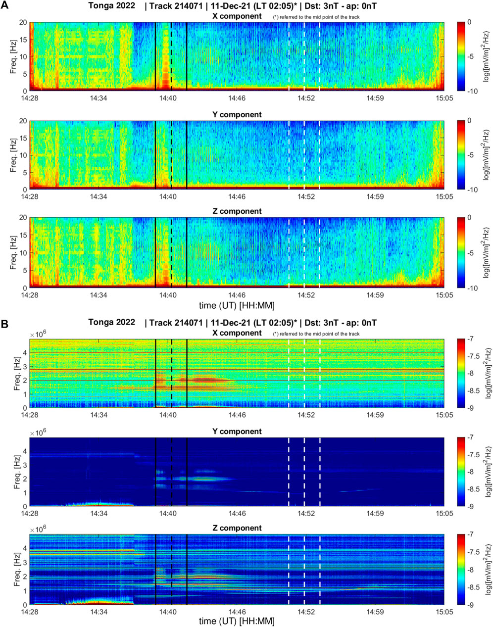
FIGURE 11. Dynamic spectra of the X, Y, and Z electric field components from CSES-01 on 11 December 2021 (orbit 214071) in the frequency range DC-20 Hz (A) and DC-5 MHz (B). The solid black vertical lines indicate the limits of the Dobrovolsky area; the inner black dashed line corresponds to the time of the minimum distance between the epicentre and the orbit; white dashed lines indicate the region with magnetically conjugate latitude with respect to the Dobrovolsky area.

3.3.4 Relevant electron losses

The analysis of the >40 keV precipitating electrons, by using NOAA satellites 15, 18 and 19 and MetOP 1, 2, and 3, is shown in Figure 12 for the time interval June 9–16, 2019. In this investigation, we selected only time intervals when all satellites are in the latitudinal and longitudinal ranges |lat|<45° and 170°<lon<230° E, respectively. Moreover, we restricted the analysis to the time interval preceding the seismic event, whose magnetic local time (MLT) falls in the range 06–13 MLT. To control electron signatures from South Atlantic Anomaly (SAA), we partially included regions on the SAA external border characterised by a total magnetic field lower than 20,100 nT, whereas the SAA boundary was identified in past works by a threshold of 20,500 nT at NOAA altitudes (Fidani, 2015). The McIlwain parameter was always limited at L-shell<2 to exclude external radiation belts. Two main peaks are detected: the first one occurring at the end of day 9 is attributable to the enhanced geomagnetic activity, while the second one occurring at the end of day 15 follows a few days of geomagnetic quiet time interval.

FIGURE 12

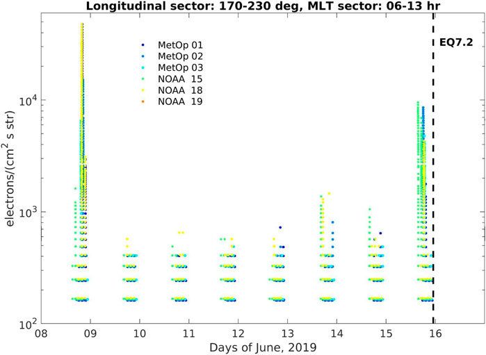
FIGURE 12. The significant electron (>40 keV) loss phenomena observed by the 0° telescope as seen on-board the selected LEO satellites during June 8–16, 2019 longitudinal sector 170°–230° E and in the range 06:00–13:00 MLT; the Kermadec seismic event is marked by vertical dashed black line. For distinguishing each satellite measurement, the electron flux counts are shifted by fixed quantities 0, 2, 4, and 6 electrons/(cm² s str) for MetOp 1, 2, 3, NOAA 15, 18, respectively.

From Figure 12 it is however difficult to investigate the longitudinal dependencies of such phenomena, therefore we repeated the same investigations by dividing the whole longitudinal sector 170°–290° E in four different sub-sectors, each one 30° large. Figure 13A reported the precipitating electron counts as a function of latitude and time in the whole longitudinal range here investigated: it represents a detailed version of Figure 12. The detailed investigation on different longitudinal sectors (Figures 13B–E) revealed that the observed increased precipitating electron fluxes during 15 June 2019, few hours before the earthquake, is well recognizable in the longitudinal sector 200°–230° E with a maximum flux of ∼9,600 electrons/(cm² s str) at 15:32 UT. Specifically, Figure 13C shows the end of the electron precipitation phenomena which disappears shortly before the strong earthquake around 18 UT. For what concerns the starting time, Figure 13D shows the precipitation phenomena through the sector 230°–260° E already soon after the 13 UT interval. It was observed around 30° further east which means that it went through the sector 200°–230° E about 1 hour before. In fact, electron drift periods Td depend on energy E and L-shell according to (Walt, 1994):

$Td=1.05/\left[EL\left(1+0.43\sin {\alpha }_{eq}\right)\right],(4)$

where ${\alpha }_{eq}$ is the equatorial pitch angle and E = 40 keV is the energy where electrons detections are concentrated, proved to be around 30° for hour. Note that all the considered electron precipitations occurred east from the Kermadec longitude, according to the eastward electron drift motion. Thus, if the precipitation was probably induced above the EQ epicentre, which is around another 1 hour of electron drift motion, it should have gone at least 7 h before lasting at least 4 h. Unfortunately, the satellite positions do not allow us to visualise the beginning time of the same phenomena. Even in the sector 230°–260° E (Figure 13D), three comparable maximum fluxes of ∼20,000, 15,100 and 21,250 electrons/(cm² s str), at 15:29:41 UT on June 13, at 15:18 UT on June 14, and 16:47 UT on 15 June 2019, were reached. These events can be probably attributable to the geomagnetic activity enhanced during June 13–14. Furthermore, the occurred enhanced fluxes between 11:00 and 15:00 UT along all the days between 9 and 15 June are attributable to non-precipitating phenomena to the internal border of SAA (Figure 13E). Conversely, in the remote (westward) longitudinal sector (Figure 13B) the electron fluxes were quite the same over all days. From the above observations, the sectors <200° E and >260° E are not further considered in our discussions.

FIGURE 13

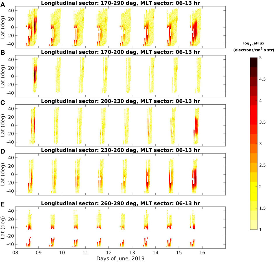
FIGURE 13. The significant electron loss phenomena (>40 keV, colour scales) observed by the 0° telescope as seen on-board the selected LEO satellites during June 8–16, 2019, and in the range 06:00–13:00 MLT. From top to bottom: the electron flux for the larger longitudinal sector 170°–290° E (A) and for each longitudinal sub-sector 170°–200° E (B), 200°–230° E (C), 230°–260° E (D), and 260°–290° E (E). White regions correspond to unselected time intervals and/or data gaps. During the whole June 16 all satellite data were unavailable. As for the selection method, it is evident the effect of the peripheral region of SAA in the last panel (E).

We also verified the possible contaminations of POES electron flux measurements due to Solar Energetic Particle (SEP) from the Energetic Proton, Electron, and Alpha Detector (EPEAD) experiment at 5 min time resolution (Bruno, 2017), and X-ray flux events at 1 min time resolution, part of the Space Environment Monitor (SEM) instrumental package (Bornmann et al., 1996), installed on board GOES satellite (https://data.ngdc.noaa.gov/). In this regard, we analysed the GOES 15 (operating on June 2019) and GOES 16 (operating on January 2021) X-ray flux in both short wavelength channel irradiance (0.05–0.4 nm) and long wavelength channel irradiance (0.1–0.8 nm), as well as the three proton flux channels (>10, >50, and >100 MeV) for GOES 15, and in 13 different channels in the range ∼1–330 MeV for GOES 16, respectively. The results shown in the S4 of Supplementary Material, confirm the absence of both SEP and solar flare during the examined time interval. Figure 14.

FIGURE 14

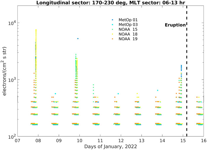
FIGURE 14. The significant electron (>40 keV) loss phenomena observed by the 0° telescope as seen on-board the selected LEO satellites during January 7–15, 2022 longitudinal sector 170°–230° E and in the range 06:00–13:00 MLT; the Tonga eruption is marked by vertical dashed black line. For distinguishing each satellite measurement, the electron flux counts are shifted by fixed quantities 0, 2, 4, and 6 electrons/(cm² s str) for MetOp 1, 3, NOAA 15, 18 and 19, respectively. MetOp 2 data were absent for this time interval.

Same investigations were conducted for the HTHH eruption which occurred in January 2022. In this case study, only data from MetOp 1 and 3, NOAA 15, 18 and 19 satellites are available. Intense electron fluxes up to $5\times {10}^3$ electrons/(cm² s sr) in the loss cone were observed from all the operating satellites towards the end of January 9 (i.e. 6 days before the eruption) and 15 (i.e., the day of the eruption). During these dates recovery phases of the geomagnetic field were observed as shown in Supplementary Figure S2C of Supplementary Material. Unfortunately, the intense recovery phase during January 15 started a few hours before the main phase of the eruption and continued the hours of the main lightning occurrence that followed the explosion (Nickolaenko et al., 2022). As ap index reaches a maximum value of 67 nT, the geomagnetic field variations are able to induce electron losses and, at the same time, to mask the possible effects on electron motion due to electromagnetic emissions linked to significant lightning activity of the volcanic plume. The electron losses observed on January 9 occurred during a less intense recovery phase. Nevertheless, with Dst around −30 nT, they were deemed capable to induce electron losses (Fidani, 2015). Several Sudden Ionospheric Disturbances (SIDs) with magnitudes between 1 and 3 were observed on January 13, 14 and 15 (see the list of SIDs in Supplementary Table S2 and solar flares in Supplementary Figure S5 of Supplementary Material). For what concerns the most intense electron precipitation on January 7 (i.e. 8 days before the major eruption), the flux reached values a little lower than 10⁴ electrons/(cm² s str) towards the end of the day. This day was completely quiet from the geomagnetic point of view, while the flare activity on the Sun photosphere produced a type B event revealed from GOES satellite, but no SIDs were reported for this day. The same precipitation event is even better described in Figure 15B, appearing at longitudes between 170° and 200° E. For this last electron precipitation, a possible origin is not yet clear, and we cannot exclude that it could have a link to the preparation phase of the eruption.

FIGURE 15

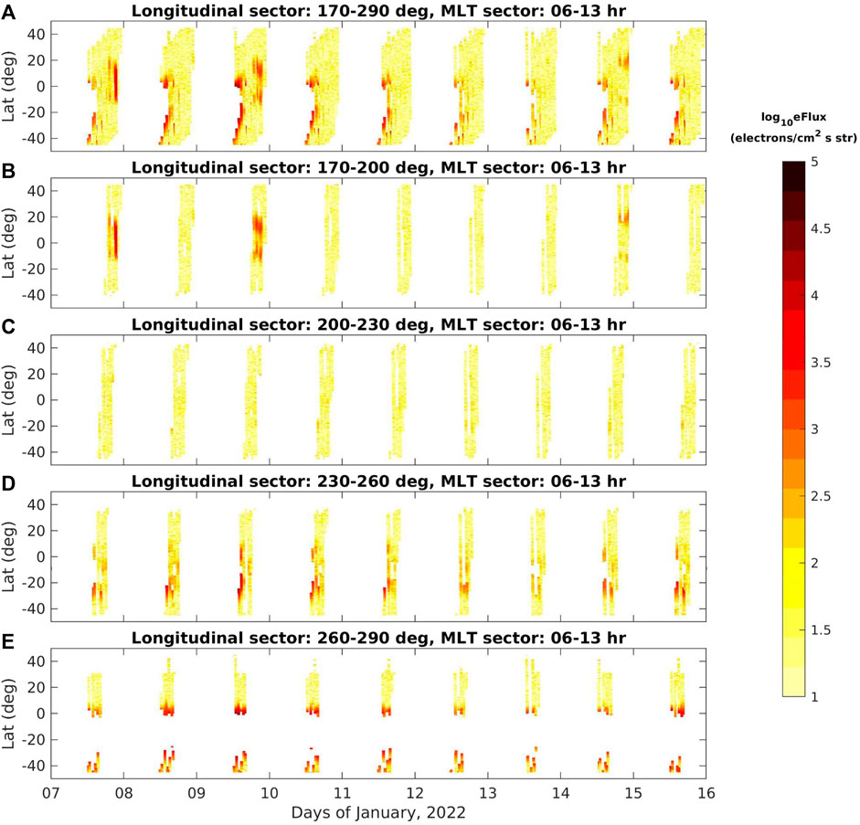
FIGURE 15. The significant electron loss phenomena (>40 keV, colour scales) observed by the 0° telescope as seen on-board the selected LEO satellites during January 10–16, 2022, and in the range 06:00–13:00 MLT. From top to bottom: the electron flux for the larger longitudinal sector 170°–290° E (A) and for each longitudinal sub-sector 170°–200° E (B), 200°–230° E (C), 230°–260° E (D), and 260°–290° E (E). As for the selection method, the peripheral region of SAA in the last panel (E) is highlighted.

4 Discussion

The seismic (Kermadec Islands EQ) and volcanic (HTHH eruption) events have been analysed here with a multi-parametric and multi-layer approach. Starting with lithospheric analysis, we identify an acceleration of the seismicity from 180 days before the Kermadec EQ and a lower acceleration starting from 120 days before the Hunga Tonga eruption. The contributing impact of both analyses is the accuracy of the predicted magnitudes provided using the R-AMR method: M 7.1–7.4 for the seismic event and the associated M 6.4–6.7 for the eruption, an intermediate magnitude between the equivalent values corresponding to the energy released in the lithosphere (M 5.8–6) and in the atmosphere (M 7). From atmospheric data, considering different parameters for both events, we put in evidence several anomalies. In detail, before Kermadec Islands EQ we found: AOD appears first around 104 days before the event, followed by SKT and TCWV at 94–93 days before the EQ. Other single anomalies were found in AOD, TCWV and OLR but it is really interesting that 16 days before the EQ all the atmospheric parameters show an anomalous value. On the other hand, for HTHH eruption, the OLR presents various a few day-persistent anomalies starting from 82 days before the event, followed by cloud cover, 2 mT and SKT in temporal order (67, 50, 49 days before the eruption, respectively). Passing to analyse the different components of the magnetic field from satellite data (Swarm and CSES-01), we notice an interesting anomaly on Y-component revealed from all satellites 110 days before the seismic event; while just a weak signal appeared on the first difference of total intensity on the eruption day. Also the electron density analysis shows anomalies possibly related to the events: for Kermadec EQ at 119 days before and for the HTHH at the eruption day.

The spectral investigation of magnetic field variations in the ULF (1–150 mHz) frequency range for Kermadec Islands shows clear correspondence with that found for the Tonga eruption in D’Arcangelo et al. (2022): a) higher power spectral density at lower satellite altitude; b) same broad-band spectral enhancement symmetrical around the equatorial region; c) a spatial concentration of power around the west pacific ridge. Same conclusion for previous investigation of the HTHH eruption can be made, reinforcing previously postulated hypothesis: a) now it is clear that the observed ULF fluctuations are not mainly related to external sources, which are essentially linked to the solar wind-magnetosphere interactions; b) the common Kermadec-Tonga ULF power enhancement in a large area around both sites and the independence from local time suggest that the revealed signals are probably linked to a great deep structure, plausibly inside the lithosphere. In addition, the latter behaviour also excludes significant upstream waves related contamination, mainly expected in the morning hours, given the typical spiral orientation of the IMF (e.g., Vellante et al., 1989; De Lauretis et al., 2010). However, from this and previous investigations, it is not clear if possible precursors of extreme events exist as magnetic fluctuations in the ULF range.

For the Kermadec Island event the magnetic field observations in the ULF band from CSES-01 satellite show the emergence of a sparse energy content at frequencies below about 20 Hz in the Dobrovolsky area, as well as in other areas in the same latitude range. Although it emerges on all components, its greater evidence on the Y-East component suggests its internal origin.

For both events we also analysed the electric field from the EFD in a wide frequency band spanning from 6 Hz to 3.5 MHz. For the Kermadec EQ we put in evidence a persistent power enhancement at about 20 kHz emerging within the Dobrovolsky area during local nighttime, both before and after the EQ. For what HTHH volcanic eruption concerns, the most remarkable feature is a “smiley-like” signal in the VLF band emerging, within the Dobrovolsky area, 10 h after the main eruption. This signal, not recorded in the other analysed days, closely resembles a VLF saucer (Parrot et al., 2011; Moser et al., 2021), although we are in a completely different region with respect to the auroral region, where saucers have been typically seen. Moser et al. (2021) also specified that such kinds of signals can come both from sources above the satellite as well as below. A few days prior to the event, the ULF band spectrograms of the electric field in the Dobrovolsky area exhibit a signal resembling a “pinnacle”. This signal represents a brief increase in power across the entire frequency band (f<20 Hz), with diminishing power as the frequency increases. Specifically, this characteristic is noticeable on December 11 (35 days before the eruption), 16 (30 days before), and 21 (25 days before), 2021, at local nighttime. Although this feature persists on most days between December 11 and 21, as well as the preceding and subsequent days, it is particularly prominent during those three dates, separated by 5 days, which coincides with the satellite orbit’s revisiting period, suggesting that such signals were emitted from the same region in all three cases. No corresponding signal is detected in the other frequency bands, ruling out the possibility of it being a signature of a lightning strike. A similar phenomenology, for slightly higher contiguous frequencies, is described in the recent paper by Zong et al. (2022), who analysed CSES-01 EFD data in the search of abnormal electromagnetic emissions associated with seismic activity. Following these “pinnacle” signals, there is a subsequent broadband signal at approximately 10 Hz. Additionally, a similar concentration of energy can be observed at the highest frequencies, around 2 MHz.

Regarding the examined precipitating electron flux, we found that during the time interval June 9–16, 2019 and in the longitudinal sector 200°–230° E an intense electron precipitation phenomenon was identified on June 15 at 15:23 UT (maximum flux of ∼10,000 electrons/(cm²·s·str)) approximately 7 h before Kermadec Islands EQ. For the examined time interval, the geomagnetic conditions were quiet, as testified by the ap geomagnetic index (Supplementary Figure S2B). Nevertheless, all satellites detected very intense electron fluxes in the loss cone. Further investigations conducted by using X-ray sensor and high energy (>10 Mev) proton detectors on board the geosynchronous satellites GOES 15 (Supplementary Figure S4) clearly indicate that both SEP and solar flares events are absent during the examined time interval; therefore, the observed electron losses occurring a few hours before the main shock are probably related to the seismic event. In the next longitudinal sector 230°–260° E, enhanced electron fluxes were detected also during the middle day of 13 and 14 June, which seem to be attributable to the increased geomagnetic activity. Regarding the Tonga event, the same investigations were conducted by using GOES 16 satellite. However, due to the higher geomagnetic activity during January 2022 (Supplementary Figure S2C, D), and to the observed three C-class flares and few minor B-class flares (Supplementary Figure S5), nothing can be concluded regarding the possible relationship between the volcano eruption and the observed electron flux peaks, although SEP events were absent. Regarding the notable electron losses observed on 7 January 2022 at longitudes between 170° and 200° E, a possible link to the preparation phase of the eruption cannot be excluded.

The anomalies registered and investigated before the seismic and the volcanic events are resumed in Table 1, showing two kinds of LAIC mechanisms: one, evidenced in orange columns, practically direct from lithosphere to ionosphere so probably of electro-magnetic nature. The second kind, referred to the other columns of anomalies, represents a secondary-diffused coupling that lasts about 3 months for both case studies analysed. Although the detected anomalies could appear random fluctuations, their statistical significance to be outliers is really high (it overpasses twice the standard deviation), supporting them as potential precursors. Moreover, the temporal sequence of all these anomalies together confirms a general distribution from lithosphere to atmosphere and ionosphere, in accordance with a possible diffusive coupling mechanism at the basis of LAIC models, despite a few anomalies also showing a direct coupling.

TABLE 1

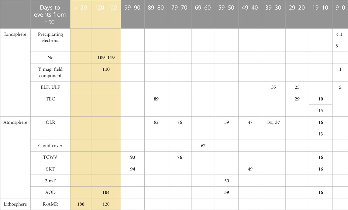
TABLE 1. Multi-precursor anomalies and their occurrence in terms of the day to the event (Kermadec Islands EQ anomalies in bold black, Hunga Tonga eruption anomalies in light black). The orange columns represent an almost direct LAIC. The rest of anomalies represents a secondary-diffused coupling that lasts about 3 months for both geophysical events.

5 Conclusion

In this paper, we conducted a comparative analysis of two significant geophysical events that occurred within a similar tectonic context but displayed distinct external manifestations at Earth’s surface: a strong seismic event (2019 Kermadec Islands EQ) and a powerful volcanic eruption (2022 HTHH eruption). Our objective was to identify the main similarities and differences between these events.

In this work, we reported evidence about the thermodynamic interaction between a stiff lithosphere and a more malleable asthenosphere inside the Kermadec-Tonga region. The results obtained from the analysis indicate the presence of two distinct types of coupling. The first kind suggests a direct connection between the lithosphere and the ionosphere, possibly of electromagnetic or mechanical origin. The second type of coupling is characterised by a secondary-diffused nature, lasting around 3 months for both case studies examined.

We employed a consistent multi-parametric and multi-layer approach, typically utilised for identifying a lithosphere-atmosphere-ionosphere coupling (LAIC) during the preparatory phase of both events. The analysis was characterised to be multidisciplinary and multiscale in space and time, exploring the behaviour of several different parameters in lithosphere, atmosphere and ionosphere and covering a wide range of temporal and spatial scales.

Considering the total energy released by these events, both had similar strength, although the energy was released differently: The Kermadec Islands EQ primarily released its energy within the lithosphere and partly in the atmosphere; conversely, the HTHH eruption predominantly released its energy in the atmosphere and partially within the lithosphere. Despite the significant disparities between these geophysical events, we discovered remarkable similarities in the occurrence of anomalies within the lithosphere, atmosphere, and ionosphere, with most anomalies appearing from bottom to top. On the other hand, the main differences can be attributed to the distinct phenomena preceding the earthquake and volcanic eruption.

In conclusion, the observed similarities in the effects of these two geophysical events can be explained by their representation of slightly different manifestations of releasing substantial energy resulting from a shared geodynamic origin. This origin arises from the thermodynamic interplay between a rigid lithosphere and a softer asthenosphere within the Kermadec-Tonga subduction zone, which forms the underlying tectonic context.

Data availability statement

The original contributions presented in the study are included in the article/Supplementary Materials, further inquiries can be directed to the corresponding author.

Author contributions

SD: Conceptualization, Formal Analysis, Investigation, Supervision, Visualization, Writing–original draft, Writing–review and editing. MR: Conceptualization, Data curation, Formal Analysis, Investigation, Methodology, Software, Supervision, Validation, Visualization, Writing–original draft, Writing–review and editing. AD: Conceptualization, Data curation, Formal Analysis, Funding acquisition, Investigation, Methodology, Project administration, Resources, Software, Supervision, Validation, Visualization, Writing–original draft, Writing–review and editing. LP: Conceptualization, Data curation, Formal Analysis, Funding acquisition, Investigation, Methodology, Project administration, Resources, Supervision, Validation, Visualization, Writing–review and editing. GC: Data curation, Formal Analysis, Investigation, Methodology, Software, Visualization, Writing–original draft, Writing–review and editing. MS: Conceptualization, Data curation, Formal Analysis, Funding acquisition, Investigation, Methodology, Project administration, Resources, Software, Supervision, Validation, Visualization, Writing–original draft, Writing–review and editing. AP: Data curation, Formal Analysis, Investigation, Methodology, Software, Validation, Visualization, Writing–original draft, Writing–review and editing. CF: Data curation, Formal Analysis, Investigation, Methodology, Software, Validation, Visualization, Writing–original draft, Writing–review and editing. DS: Data curation, Formal Analysis, Investigation, Methodology, Software, Validation, Visualization, Writing–original draft, Writing–review and editing. SL: Formal Analysis, Investigation, Methodology, Software, Validation, Visualization, Writing–original draft, Writing–review and editing. DD: Formal Analysis, Investigation, Methodology, Software, Validation, Visualization, Writing–original draft, Writing–review and editing.

Funding

The authors declare financial support was received for the research, authorship, and/or publication of this article. This work is financially supported by INGV-MUR Project Pianeta Dinamico—“The Working Earth”—theme 5—CHOPIN 2023 and FURTHER projects. Some authors received funds from the “Limadou-Scienza +” Project funded by the Italian Space Agency.

Acknowledgments

We would like to thank GeoNet (NZ) for GNSS data and the Kyoto World Data Center for Geomagnetism (http://wdc.kugi.kyoto-u.ac.jp/) to furnish geomagnetic data indices. Satellite measurements of solar wind and interplanetary magnetic field conditions are provided by OMNIWeb (https://cdaweb.gsfc.nasa.gov/) and GNSS data are furnished by GeoNet GNSS/GPS network (https://www.geonet.org.nz/). We also thank ESA for providing the Swarm satellite data and the CNSA (Chinese National Space Administration) to allow us to use CSES-01 satellite data (www.leos.ac.cn). Finally, we thank the National Oceanic and Atmospheric Administration (NOAA) for furnishing POES SEM satellites data and the principal investigators and teams of the EPS and EPEAD experiments on GOES satellites (https://data.ngdc.noaa.gov/). Data from ETOPO1 1 Arc-Minute Global Relief Model are available at https://www.ngdc.noaa.gov/mgg/global/relief/ETOPO1/data/ice_surface/grid_registered/binary/, while the Global Self-consistent, Hierarchical, High-resolution Geography Database (GSHHG) is available at http://www.ngdc.noaa.gov/mgg/shorelines/data/gshhs/, both provided by the National Oceanic and Atmospheric Administration (NOAA). The ECMWF data were generated using Copernicus Atmosphere Monitoring Service (2023) information. We would also like to thank Dr. Adriano Nardi (INGV, Italy) and Dr. Saioa A. Campuzano (UCM, Spain) for some fruitful discussions.

Conflict of interest

The authors declare that the research was conducted in the absence of any commercial or financial relationships that could be construed as a potential conflict of interest.

Publisher’s note

All claims expressed in this article are solely those of the authors and do not necessarily represent those of their affiliated organizations, or those of the publisher, the editors and the reviewers. Any product that may be evaluated in this article, or claim that may be made by its manufacturer, is not guaranteed or endorsed by the publisher.

Supplementary material

The Supplementary Material for this article can be found online at: https://www.frontiersin.org/articles/10.3389/feart.2023.1267411/full#supplementary-material

References

Adil, M. A., Şentürk, E., Pulinets, S. A., and Amory-Mazaudier, C. (2021). A lithosphere-atmosphere-ionosphere coupling phenomenon observed before M7.7 Jamaica earthquake. Pure Appl. Geophys. 178 (10), 3869–3886. doi:10.1007/s00024-021-02867-z

CrossRef Full Text | Google Scholar

Aleksandrin, S. Y., Galper, A. M., Grishantzeva, L. A., Koldashov, S. V., Maslennikov, L. V., Murashov, A. M., et al. (2003). High-energy charged particle bursts in the near-earth space as earthquake precursors. Ann. Geophys. 21, 597–602. doi:10.5194/angeo-21-597-2003

CrossRef Full Text | Google Scholar

Alken, P., Thébault, E., Beggan, C. D., Amit, H., Aubert, J., Baerenzung, J., et al. (2021). International geomagnetic reference field: the thirteenth generation. Earth Planets Space 73, 49. doi:10.1186/s40623-020-01288-x

CrossRef Full Text | Google Scholar

Amante, C., and Eakins, B. W. (2009). ETOPO1 1 Arc-Minute global Relief model: procedures, data sources and analysis. NOAA technical memorandum NESDIS NGDC-24. Available at: https://www.ngdc.noaa.gov/mgg/global/relief/ETOPO1/docs/ETOPO1.pdf.

Google Scholar

Battiston, R., and Fidani, C. (2010). Correlations between NOAA satellite particle bursts and strong earthquakes. Geophys. Res. Abstr. 12. EGU 2010-9093.

Google Scholar

Battiston, R., and Vitale, V. (2013). First evidence for correlations between electron fluxes measured by NOAA-POES satellites and large seismic events. Nucl. Phys. B - Proc. Suppl. 243-244, 249–257. Proceedings of the IV International Conference on Particle and Fundamental Physics in Space. doi:10.1016/j.nuclphysbps.2013.09.002

CrossRef Full Text | Google Scholar

Bornmann, P. L., Speich, D., Hirman, J., Matheson, L., Grubb, R., Garcia, H., et al. (1996). “GOES x-ray sensor and its use in predicting solar-terrestrial disturbances,” in Proceedings volume 2812, GOES-8 and beyond;. Editor E. R. Washwell (Denver, CO, United States: SPIE), 291–298. doi:10.1117/12.254076

CrossRef Full Text | Google Scholar

Bowman, D. D., Ouillon, G., Sammis, C. G., Sornette, A., and Sornette, D. (1998). An observational test of the critical earthquake concept. J. Geophys. Res. 103 (10), 24359–24372. doi:10.1029/98JB00792

CrossRef Full Text | Google Scholar

Bruno, A. (2017). Calibration of the GOES 13/15 high-energy proton detectors based on the PAMELA solar energetic particle observations. Space weather. 15, 1191–1202. doi:10.1002/2017SW001672

CrossRef Full Text | Google Scholar

Campbell, W. H. (2003). Comment on “Survey tracks current position of South Magnetic Pole” and “Recent acceleration of the north magnetic pole linked to magnetic jerks”. Eos Trans. AGU 84 (5), 40. doi:10.1029/2003EO050008

CrossRef Full Text | Google Scholar

Cao, J., Zeng, L., Zhan, F., Wang, Z. G., Wang, Y., Chen, Y., et al. (2018). The electromagnetic wave experiment for CSES mission: search coil magnetometer. Sci. China Technol. Sci. 61, 653–658. doi:10.1007/s11431-018-9241-7

CrossRef Full Text | Google Scholar

Cesaroni, C., Spogli, L., Alfonsi, L., De Franceschi, G., Ciraolo, L., Monico, J. F. G., et al. (2015). L-band scintillations and calibrated total electron content gradients over Brazil during the last solar maximum. J. Space Weather Space Clim. 5, A36. doi:10.1051/swsc/2015038

CrossRef Full Text | Google Scholar

Chernogor, L. F., and Rozumenko, V. T. (2008). Earth – atmosphere – geospace as an open nonlinear dynamical system. Radio Phys. Radio Astronomy 13, 120–137. Available at: http://rpra-journal.org.ua/index.php/ra/article/view/563. doi:10.15407/rpra

CrossRef Full Text | Google Scholar

Chernogor, L. F., and Shevelev, M. B. (2022). “Statistical characteristics of atmospheric waves, generated by the explosion of the Tonga volcano on January 15, 2022,” in Astronomy and Space Physics. Book of Abstracts. International Conference, Kyiv, Ukraine, October 18-21, 2022, 85–86.

Google Scholar

Chernogor, L. F. (2011). The earth-atmosphere-geospace system: main properties and processes. Int. J. Remote Sens. 32 (11), 3199–3218. doi:10.1080/01431161.2010.541510

CrossRef Full Text | Google Scholar

Choi, J. M., Lin, C., Rajesh, P. K., Lin, J. T., Chou, M., Kwak, Y. S., et al. (2023). Giant ionospheric density hole near the 2022 Hunga-Tonga volcanic eruption: multi-point satellite observations. Preprint from Research Square. Avaialable at: https://doi.org/10.21203/rs.3.rs-2759269/v1 (Accessed April 18, 2023).

Google Scholar

Cianchini, G., De Santis, A., Di Giovambattista, R., Abbattista, C., Amoruso, L., Campuzano, S. A., et al. (2020). Revised accelerated moment release under test: fourteen worldwide real case studies in 2014–2018 and simulations. Pure Appl. Geophys. 177, 4057–4087. doi:10.1007/s00024-020-02461-9

CrossRef Full Text | Google Scholar

Ciraolo, L., Azpilicueta, F., Brunini, C., Meza, A., and Radicella, S. M. (2007). Calibration errors on experimental slant total electron content (TEC) determined with GPS. J. Geod. 81 (2), 111–120. doi:10.1007/s00190-006-0093-1

CrossRef Full Text | Google Scholar

D’Arcangelo, S., Bonforte, A., De Santis, A., Maugeri, S. R., Perrone, L., Soldani, M., et al. (2022). A multi-parametric and multi-layer study to investigate the largest 2022 Hunga Tonga-Hunga Ha’apai eruptions. Remote Sens. 14, 3649. doi:10.3390/rs14153649

CrossRef Full Text | Google Scholar

Davis, G. (2007). History of the NOAA satellite program. J. Appl. Remote Sens. 1, 012504. doi:10.1117/1.2642347

CrossRef Full Text | Google Scholar

De Lauretis, M., Francia, P., Regi, M., Villante, U., and Piancatelli, A. (2010). Pc3 pulsations in the polar cap and at low latitude. J. Geophys. Res. 115, A11223. doi:10.1029/2010JA015967

CrossRef Full Text | Google Scholar

De Santis, A., Cianchini, G., and Di Giovambattista, R. (2015). Accelerating moment release revisited: examples of application to Italian seismic sequences. Tectonophysics 639, 82–98. doi:10.1016/j.tecto.2014.11.015

CrossRef Full Text | Google Scholar

De Santis, A., Marchetti, D., Spogli, L., Cianchini, G., Pavón-Carrasco, F. J., De Franceschi, G., et al. (2019). Magnetic field and electron density data analysis from Swarm satellites searching for ionospheric effects by great earthquakes: 12 case studies from 2014 to 2016. Atmosphere 10, 371. doi:10.3390/atmos10070371

CrossRef Full Text | Google Scholar

De Santis, A., Perrone, L., Calcara, M., Campuzano, S. A., Cianchini, G., D’Arcangelo, S., et al. (2022). A comprehensive multiparametric and multilayer approach to study the preparation phase of large earthquakes from ground to space: the case study of the June 15 2019, M7.2 Kermadec Islands (New Zealand) earthquake. Remote Sens. Environ. 283, 113325. doi:10.1016/j.rse.2022.113325

CrossRef Full Text | Google Scholar

Diego, P., Huang, J., Piersanti, M., Badoni, D., Zeren, Z., Yan, R., et al. (2021). The electric field detector on board the China seismo electromagnetic satellite—in-orbit results and validation. Instruments 5, 1. doi:10.3390/instruments5010001

CrossRef Full Text | Google Scholar

Dobrovolsky, I. P., Zubkov, S. I., and Miachkin, V. I. (1979). Estimation of the size of earthquake preparation zones. Pure Appl. Geophys. 117, 1025–1044. doi:10.1007/bf00876083

CrossRef Full Text | Google Scholar

Fidani, C., Battiston, R., and Burger, W. J. (2010). A study of the correlation between earthquakes and NOAA satellite energetic particle bursts. Remote Sens. 2, 2170–2184. doi:10.3390/rs2092170

CrossRef Full Text | Google Scholar

Fidani, C. (2018). Improving earthquake forecasting by correlations between strong earthquakes and NOAA electron bursts. TAO 29 (2), 117–130. doi:10.3319/TAO.2017.10.06.01

CrossRef Full Text | Google Scholar

Fidani, C. (2015). Particle precipitation prior to large earthquakes of both the sumatra and philippine regions: A statistical analysis. J. Asian Earth Sci. 114, 384–392. doi:10.1016/j.jseaes.2015.06.010

CrossRef Full Text | Google Scholar

Fidani, C. (2020). Probability, causality and false alarms using correlations between strong earthquakes and NOAA high energy electron bursts. Ann. Geophys. 63 (5), 543. doi:10.44101/ag-7957

CrossRef Full Text | Google Scholar

Fidani, C. (2022). The conditional probability of correlating east pacific earthquakes with NOAA electron bursts. Appl. Sci. 12, 10528. doi:10.3390/app122010528

CrossRef Full Text | Google Scholar

Fidani, C. (2021). West pacific earthquake forecasting using NOAA electron bursts with independent L-shells and ground-based magnetic correlations. Front. Earth Sci. Sect. Environ. Inf. Remote Sens. 9, 673105. doi:10.3389/feart.2021.673105

CrossRef Full Text | Google Scholar

Francia, P., De Lauretis, M., and Regi, M. (2013). ULF fluctuations observed along the SEGMA array during very low solar wind density conditions. Planet. Space Sci. 81, 74–81. doi:10.1016/j.pss.2013.03.008

CrossRef Full Text | Google Scholar

Freund, F. (2011). Pre-earthquake signals: underlying physical processes. J. Asian Earth Sci. 41 (4-5), 383–400. doi:10.1016/j.jseaes.2010.03.009

CrossRef Full Text | Google Scholar

Gutenberg, B., and Richter, C. F. (1954). Seismicity of the earth and associated phenomena. 2nd ed. Princeton, NJ, USA: Princeton University Press.

Google Scholar

Han, S. C., McClusky, S., Mikesell, T. D., Rolland, L., Okal, E., and Benson, C. (2023). CubeSat GPS observation of traveling ionospheric disturbances after the 2022 Hunga-Tonga Hunga-Ha’apai volcanic eruption and its potential use for tsunami warning. Earth Space Sci. 10, e2022EA002586. doi:10.1029/2022EA002586

CrossRef Full Text | Google Scholar

Hayakawa, M., and Molchanov, O. A.NASDA/UEC Team (2004). Summary report of NASDA’s earthquake remote sensing frontier project. Phys. Chem. Earth 29, 617–625. doi:10.1016/j.pce.2003.08.062

CrossRef Full Text | Google Scholar

Korepanov, V., Hayakawa, M., Yampolski, Y., and Lizunov, G. (2009). AGW as a seismo-ionospheric coupling responsible agent. Phys. Chem. Earth 34, 485–495. doi:10.1016/j.pce.2008.07.014

CrossRef Full Text | Google Scholar

Kumar, S., Singh, P. K., Kumar, R., Singh, A., and Singh, R. (2021). Ionospheric and atmospheric perturbations due to two major earthquakes (M > 7.0). J. Earth Syst. Sci. 130 (3), 149–215. doi:10.1007/s12040-021-01650-x

CrossRef Full Text | Google Scholar

Li, W., Guo, J., Yue, J., Shen, Y., and Yang, Y. (2016). Total electron content anomalies associated with global VEI4+ volcanic eruptions during 2002-2015. J. Volcanol. Geotherm. Res. 325, 98–109. doi:10.1016/j.jvolgeores.2016.06.017

CrossRef Full Text | Google Scholar

Liu, Q., De Santis, A., Piscini, A., Cianchini, G., Ventura, G., and Shen, X. (2020). Multi-parametric climatological analysis reveals the involvement of fluids in the preparation phase of the 2008 Ms 8.0 wenchuan and 2013 Ms 7.0 lushan earthquakes. Remote Sens. 12, 1663. doi:10.3390/rs12101663

CrossRef Full Text | Google Scholar

Madonia, P., Bonaccorso, A., Bonforte, A., Buonocunto, C., Cannata, A., Carleo, L., et al. (2023). Propagation of perturbations in the lower and upper atmosphere over the central mediterranean, driven by the 15 january 2022 Hunga Tonga-Hunga Ha’apai volcano explosion. Atmosphere 14 (1), 65. doi:10.3390/atmos14010065

CrossRef Full Text | Google Scholar

Molchanov, O. A., and Hayakawa, M. (2008). Seismo electromagnetics and related phenomena: History and latest results. Tokyo: Terra Scientific Publishing, 189.

Google Scholar

Moser, C., LaBelle, J., Hatch, S., Moen, J. I., Spicher, A., Takahashi, T., et al. (2021). The cusp as a VLF saucer source: first rocket observations of long-duration VLF saucers on the dayside. Geophys. Res. Lett. 48, e2020GL090747. doi:10.1029/2020GL090747

CrossRef Full Text | Google Scholar

Nanjo, K. Z., and Yoshida, A. (2021). Changes in the b-value in and around the focal areas of the M6.9 and M6.8 earthquakes off the coast of Miyagi prefecture, Japan, in 2021. Earth Planets Space 73, 176. doi:10.1186/s40623-021-01511-3

CrossRef Full Text | Google Scholar

Nickolaenko, A. P., Schekotov, A. Y., Hayakawa, M., Romero, R., and Izutsu, J. (2022). Electromagnetic manifestations of Tonga eruption in Schumann resonance band. J. Atmos. Solar-Terrestrial Phys. 237, 105897. doi:10.1016/j.jastp.2022.105897

CrossRef Full Text | Google Scholar

Otsuka, S. (2022). Visualizing Lamb waves from a volcanic eruption using meteorological satellite Himawari-8. Geophys. Res. Lett. 49 (8), e2022GL098324. doi:10.1029/2022GL098324

CrossRef Full Text | Google Scholar

Parrot, M., Berthelier, J., and Brochot, J. (2011). Truncated VLF saucers observed by the low altitude satellite DEMETER. IEEE Trans. Plasma Sci. 39, 2702–2703. doi:10.1109/TPS.2011.2131682

CrossRef Full Text | Google Scholar

Pawlowicz, R. (2020). Map: A mapping package for MATLAB. Available at: http://www.eoas.ubc.ca/∼rich/map.html.

Google Scholar

Pesicek, J. D., Wellik, J. J., Prejean, S. G., and Ogburn, S. E. (2018). Prevalence of seismic rate anomalies preceding volcanic eruptions in Alaska. Front. Earth Sci. 6, 100. doi:10.3389/feart.2018.00100

CrossRef Full Text | Google Scholar

Pinheiro, K. J., Jackson, A., and Finlay, C. C. (2011). Measurements and uncertainties of the occurrence time of the 1969, 1978, 1991, and 1999 geomagnetic jerks. Geochem. Geophys. Geosyst. 12, Q10015. doi:10.1029/2011GC003706

CrossRef Full Text | Google Scholar

Piscini, A., De Santis, A., Marchetti, D., and Cianchini, G. (2017). A Multi-parametric Climatological Approach to study the 2016 Amatrice-Norcia (Central Italy) earthquake preparatory phase. Pure Appl. Geophys. 174, 3673–3688. doi:10.1007/s00024-017-1597-8

CrossRef Full Text | Google Scholar

Piscini, A., Marchetti, D., and De Santis, A. (2019). Multi-parametric climatological analysis associated with global significant volcanic eruptions during 2002-2017. Pure Appl. Geophys. 176, 3629–3647. doi:10.1007/s00024-019-02147-x

CrossRef Full Text | Google Scholar

Pulinets, S., and Ouzounov, D. (2011). Lithosphere-Atmosphere-Ionosphere Coupling (LAIC) model – an unified concept for earthquake precursors validation. J. Asian Earth Sci. 41 (4-5), 371–382. doi:10.1016/j.jseaes.2010.03.005

CrossRef Full Text | Google Scholar

Regi, M., De Lauretis, M., and Francia, P. (2014a). The occurrence of upstream waves in relation with the solar wind parameters: A statistical approach to estimate the size of the foreshock region. Planet. Space Sci. 90, 100–105. doi:10.1016/j.pss.2013.10.012

CrossRef Full Text | Google Scholar

Regi, M., De Lauretis, M., Francia, P., and Villante, U. (2014b). The propagation of ULF waves from the Earth’s foreshock region to ground: the case study of 15 february 2009. Earth Planets Space 66, 43. doi:10.1186/1880-5981-66-43

CrossRef Full Text | Google Scholar

Regi, M., Di Mauro, D., and Lepidi, S. (2021). The location of the Earth's magnetic poles from circumterrestrial observations. J. Geophys. Res. Space Phys. 126, e2020JA028513. doi:10.1029/2020JA028513

CrossRef Full Text | Google Scholar

Regi, M., Francia, P., De Lauretis, M., Glassmeier, K. H., and Villante, U. (2013). Coherent transmission of upstream waves to polar latitudes through magnetotail lobes. J. Geophys. Res. Space Phys. 118, 6955–6963. doi:10.1002/2012ja018472

CrossRef Full Text | Google Scholar

Scholz, C. H. (2015). On the stress dependence of the earthquake b value. Geophys. Res. Lett. 42 (5), 1399–1402. doi:10.1002/2014GL062863

CrossRef Full Text | Google Scholar

Schwarz-Schampera, U., Botz, R., Hannington, M., Adamson, R., Anger, V., Cormany, D., et al. (2007). Cruise report SONNE 192/2 MANGO. New Zealand: Bundesanstalt für Geowissenschaften und Rohstoffe, 92.

Google Scholar

Sgrigna, V., Carota, L., Conti, L., Corsi, M., Galper, A. M., Koldashov, S. V., et al. (2005). Correlations between earthquakes and anomalous particle bursts from SAMPEX/PET satellite observations. J. Atmos. Solar-Terrestrial Phys. 67, 1448–1462. doi:10.1016/j.jastp.2005.07.008

CrossRef Full Text | Google Scholar

Shah, M., Aibar, A. C., Tariq, M. A., Ahmed, J., and Ahmed, A. (2020). Possible ionosphere and atmosphere precursory analysis related to M_w>6.0 earthquakes in Japan. Remote Sens. Environ. 239, 111620. doi:10.1016/j.rse.2019.111620

CrossRef Full Text | Google Scholar

Shah, M., Arslan Tariq, M., and Abbas Naqvi, N. (2019). Atmospheric anomalies associated with M_w>6.0 earthquakes in Pakistan and Iran during 2010-2017. J. Atmos. Solar-Terrestrial Phys. 191, 105056. doi:10.1016/j.jastp.2019.06.003

CrossRef Full Text | Google Scholar

Shepherd, S. G. (2014). Altitude-adjusted corrected geomagnetic coordinates: definition and functional approximations. J. Geophys. Res. (Space Phys.) 119, 7501–7521. doi:10.1002/2014ja020264

CrossRef Full Text | Google Scholar

Thurin, J., Tape, C., and Modrak, R. (2022). Multi-event explosive seismic source for the 2022 M_w 6.3 Hunga Tonga submarine volcanic eruption. Seismic Rec. 2 (4), 217–226. doi:10.1785/0320220027

CrossRef Full Text | Google Scholar

Troitskaya, V. A., and Bolshakova, O. V. (1988). Diagnostics of the magnetosphere using multipoint measurements of ULF-waves. Adv. Space Res. 8, 413–425. doi:10.1016/0273-1177(88)90155-X

CrossRef Full Text | Google Scholar

Vellante, M., Villante, U., De Lauretis, M., and Cerulli-Irelli, P. (1989). An analysis of micropulsation events at a low-latitude station during 1985. Planet. Space Sci. 37, 767–773. doi:10.1016/0032-0633(89)90128-1

CrossRef Full Text | Google Scholar

Voronov, S. A., Galper, A. M., and Koldashov, S. V. (1989). Observation of high-energy charged particle flux increases in SAA region on 10 September 1985. Cosm. Res. 27, 629–631.

Google Scholar

Walt, M. (1994). Introduction to geomagnetically trapped radiation. Camb. Atmos. Space Sci. Ser. 10.

Google Scholar

Zhao, S., Shen, X., Liao, L., and Zeren, Z. (2021). A lithosphere-atmosphere-ionosphere coupling model for ELF electromagnetic waves radiated from seismic sources and its possibility observed by the CSES. Sci. China Tech. Sci. 64, 2551–2559. doi:10.1007/s11431-021-1934-5

CrossRef Full Text | Google Scholar

Zong, J., Tao, D., and Shen, X. (2022). Possible ELF/VLF electric field disturbances detected by satellite CSES before major earthquakes. Atmosphere 13, 1394. doi:10.3390/atmos13091394

CrossRef Full Text | Google Scholar