
94% of researchers rate our articles as excellent or good
Learn more about the work of our research integrity team to safeguard the quality of each article we publish.
Find out more
ORIGINAL RESEARCH article
Front. Earth Sci., 16 October 2023
Sec. Geoinformatics
Volume 11 - 2023 | https://doi.org/10.3389/feart.2023.1267386
This article is part of the Research TopicArtificial Intelligence in Remote Sensing and Geosciences: Applications for Earth ObservationsView all articles
Wave velocity profiles are significant for various fields, including rock engineering, petroleum engineering, and earthquake engineering. However, direct measurements of wave velocities are often constrained by time, cost, and site conditions. If wave velocity measurements are unavailable, they need to be estimated based on other known proxies. This paper proposes machine learning (ML) approaches to predict the compression and shear wave velocities (VP and VS, respectively) in Japan. We utilize borehole databases from two seismograph networks of Japan: Kyoshin Network (K-NET) and Kiban Kyoshin Network (KiK-net). We consider various factors such as depth, N-value, density, slope angle, elevation, geology, soil/rock type, and site coordinates. We use three ML techniques: Gradient Boosting (GB), Random Forest (RF), and Artificial Neural Network (ANN) to develop predictive models for both VP and VS and evaluate the performances of the models based on root mean squared errors and the five-fold cross-validation method. The GB-based model provides the best estimation of VP and VS for both seismograph networks. Among the considered factors, the depth, standard penetration test (SPT) N-value, and density have the strongest influence on the wave velocity estimation for K-NET. For KiK-net, the depth and site longitude have the strongest influence. The study confirms the applicability of commonly used machine-learning techniques in predicting wave velocities, and implies that exploring additional factors will enhance the performance.
Compression and shear wave velocities (VP and VS, respectively) are often employed to assess the properties of underground rock environments and to design geotechnical projects. VP and VS are significant in various fields such as rock mechanical property calculations (Chang et al., 2006; Ameen et al., 2009; Jamshidi et al., 2018; Rahman and Sarkar, 2021), pore structure identification (Eberli et al., 2003; Panza et al., 2019), lithology determination (Pickett, 1963; Deng et al., 2017), fluid saturation (Si et al., 2016; Roy et al., 2017; Ding et al., 2019), seismic liquefaction (Samui et al., 2011; Karthikeyan and Samui, 2014; Jena et al., 2023), seismic site responses, and ground motion predictions (Fiorentino et al., 2019; Harmon et al., 2019; Kim, 2019). Such wave velocities are measured by invasive tests such as down-hole test, cross-hole test, and suspension PS logging, as well as non-destructive tests such as Multichannel Analysis of Surface Wave (MASW), Spectral Analysis of Surface Wave (SASW), and Multichannel Simulation with One Receiver (MSOR). However, these tests are often constrained by time, cost, and site conditions (Hasancebi and Ulusay, 2007; Anemangely et al., 2019; Xiao et al., 2021).
To address the problems mentioned in the prior paragraph, numerous researchers have proposed indirect methods to estimate VP or VS. For instance, several studies have presented the relationships between VP and the mechanical properties of rock materials, such as uniaxial compressive strength (Pappalardo, 2015), density (Yasar and Erdogan, 2004), and porosity (Sousa et al., 2005). Various correlation models between VS and standard penetration test (SPT) resistance (N-value) have also been suggested (e.g., Ohta and Goto, 1978; Andrus et al., 2004; Akin et al., 2011; Sil and Haloi, 2017; Bajaj and Anbazhagan, 2019). For example, Kwak et al. (2015); Tsai et al. (2019) inferred VS using empirical equations conditioned on the N-value and other independent variables such as vertical effective stress and soil type. Rahimi et al. (2020) presented the effect of soil aging on SPT-VS correlations. Furthermore, researchers have predicted the time-averaged shear-wave velocity in the upper 30 m of soil deposits (VS30) based on various proxies, such as topographic slope, surface geology, elevation, and terrain type (e.g., Kottke et al., 2012; Parker et al., 2017; Kwok et al., 2018; Heath et al., 2020).
The demand for Machine learning (ML) applications has been increasing as huge volumes of data are accessible over a computer network. ML algorithms are well suited for making regression models on complex data-driven problems. Researchers have studied VP or VS estimation based on ML (e.g., Singh and Kanli, 2016; Paul et al., 2018; Anemangely et al., 2019; Dumke and Berndt, 2019; Wang and Peng, 2019; Zhang et al., 2020). In particular, Dumke and Berndt (2019) used the Random Forest (RF) regression algorithm to estimate VP as a function of depth on global marine locations. They used data from 333 boreholes and considered 38 geological variables, such as site coordinates, sediment thickness, and depth below the seafloor. They validate the ML model using 10-fold cross-validation (CV). Paul et al. (2018) used an Artificial Neural Network (ANN) algorithm on data from five wells in India to estimate the VP. Singh and Kanli (2016) used an ANN to estimate VS in an oil field located in southeastern Turkey. Anemangely et al. (2019) adopted the least square version of the support vector machine (LSSVM) algorithm combined with three optimization algorithms to predict VS using data from two oilfields located in the southwest of Iran.
This study aims to train the three ML algorithms (i.e., gradient boosting, random forest, and artificial neural network) to estimate both VP and VS in Japan. We utilize borehole databases, covering all of Japan from two seismograph networks: Kyoshin Network (K-NET) and Kiban Kyoshin Network (KiK-net). We consider various factors such as depth, N-value, density, slope angle, elevation, geology, soil/rock type, and site coordinates. We quantitatively evaluate the prediction performances of the ML-based algorithms based on five-fold cross-validation and evaluate the relative importance of the factors.
In this study, we obtained site data from two seismograph networks of Japan, Kyoshin Network (K-NET) and Kiban Kyoshin Network (KiK-net), where the National Research Institute for Earth Science and Disaster Resilience (2019) has operated since 1996. Each site of these two networks has profiles of VP, VS, and soil/rock types. In addition, the K-NET site has profiles of standard penetration test (SPT) resistance values (N-values) and density with a depth interval of 1 m. The energy efficiency is unknown for the borings at the K-NET sites (Kwak et al., 2015). Therefore, we utilized unnormalized N-values. Because of the inconsistent datasets between the two seismograph networks, we considered training the ML models for each network.
For the datasets, the velocity profile data were resampled to a depth interval of 1 m. For all of the K-NET sites, a minimum depth interval is 1 m. Furthermore, approximately 43% of KiK-net sites have minimum depth intervals of 1 m or shorter. Therefore, we consider that resampling the profile data into a depth interval of 1 m is reasonable. We also screen the suspicious profile data such as those with the velocity of zero. In addition to the depth-dependent variables provided by the networks, we also considered the following five depth-independent variables: site latitude, site longitude, geology, topographic slope angle, and elevation. The geology map was obtained from the seamless digital geological map of Japan (1:200,000) (Geological Survey of Japan, 2015), and the slope angle and elevation were obtained from the digital elevation map (DEM) of the Shuttle Radar Topography Mission (SRTM) with a resolution of 30 m. We then used the nine independent variables (i.e., site longitude, site latitude, geology, slope angle, elevation, N-value, density, depth, soil/rock type) for the K-NET, and seven (i.e., site longitude, site latitude, geology, slope angle, elevation, depth, and soil/rock type) for the KiK-net sites, as summarized in Table 1.
We considered all sites where all of the variables were available: 996 K-NET sites with 15,253 data samples for each of VP and VS and 677 KiK-net sites with 136,315 data samples for VP and 132,855 data samples for VS. The dataset information is summarized in Table 1. The considered sites (i.e., recording stations) covering Japan are shown in Figure 1.
The distributions of the numerical variables for the K-NET and KiK-net datasets are shown in Figure 2 and Figure 3, respectively. The depth to the bottom of the borehole (Dbh) at the K-NET sites ranges from 5 to 20 m, with 83% concentration at 10 m and 20 m (Figure 2A). The elevation ranges from −3 m to 1,502 m, 75% of which are positioned under 179 m, as shown in the boxplot above the histogram (Figure 2B). The slope angle ranges from 0° to 30.87°, with 75% below 5.26° (Figure 2C). The 96 outliers are observed as circular forms in each boxplot (Figures 2B, C). The N-value with depth ranges from 0 to 500 with 69% below 90, where the four outliers are observed: three of which are 375, and one is 500 (Figure 2D). The density with depth is distributed from 0.69 g/cm3 to 2.82 g/cm3 with 75% under 1.98 g/cm3, in which 306 outliers are detected (Figure 2E). The VS is distributed from 37 m/s to 2,350 m/s with 75% slower than 450 m/s (Figure 2F). The VP ranges from 140 m/s to 5,270 m/s with 75% slower than 1,800 m/s (Figure 2G). For categorical variables in K-NET sites in our dataset, 12 unique soil/rock types according to depth and 110 unique types of geology are observed.
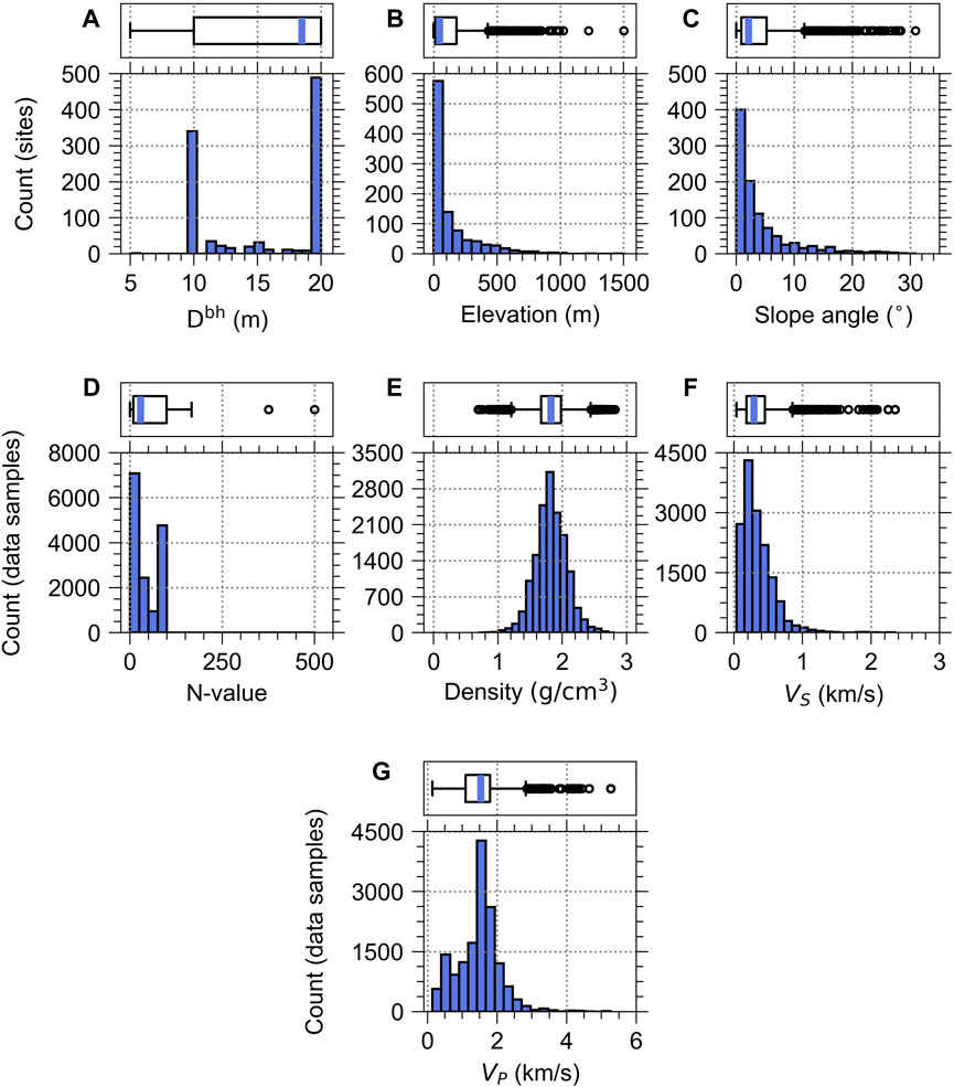
FIGURE 2. Variables distribution for K-NET dataset used in this study: (A) depth to the bottom of the borehole (Dbh), (B) elevation, (C) slope angle for the sites (i.e., 996 sites), and (D) N-value, (E) density, (F) VS, (G) VP for data samples (i.e., 15,253 data samples). In the boxplot above the histogram, the blue line represents a median value, and the box represents 25 and 75 percentiles of the data.
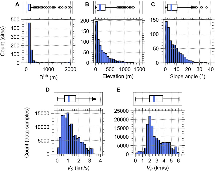
FIGURE 3. Variables distribution for KiK-net dataset used in this study: (A) depth to the bottom of the borehole (Dbh), (B) station elevation, (C) station slope angle for the sites of VP dataset (i.e., 677 sites), and (D) VS, (E) VP for data samples (i.e., 132,855 and 136,315 data samples, respectively). In the boxplot above the histogram, the blue line represents a median value, and the box represents 25 and 75 percentiles of the data.
Figure 3A depicts the Dbh of the KiK-net sites ranging from 92 m to 2,000 m, with 75% under 199 m, where 46 outliers are observed. Figure 3B presents the site elevation ranging from −5 m to 1,302 m with 75% below 330 m, where 34 outliers are detected. Figure 3C shows the slope angle that ranges from 0° to 36.23° with 75% under 10.42°, where 12 outliers are observed. Figure 3D shows the VS ranging from 20 m/s to 3,500 m/s with 75% slower than 1,720 m/s. Figure 3E presents the VP that ranges from 50 m/s to 6,100 m/s with 75% slower than 3,830 m/s. For categorical variables, soil/rock type with depth has 588 unique features, among which the features include the various combinations of several soil types, such as ‘sand and gravel’, ‘shale with gravel’, and ‘sandstone and mudstone’. Furthermore, 119 unique geological classes are observed.
The ML model uses the following variables: the depth and depth-related information (i.e., N-value, density, soil/rock type), and site information (i.e., coordinates, slope angle, elevation, geology) described in Table 1 to infer VP or VS on a specific depth (e.g., 15 m) of the site. This section describes the ML algorithms utilized for VP and VS prediction. We illustrated them using all K-NET data samples for VS as an example. We used Scikit-learn (Pedregosa et al., 2011) for the implementation of Gradient Boosting (GB) and Random Forest (RF) algorithms and the Tensorflow (Abadi et al., 2016) for the Artificial Neural Network (ANN) algorithm. Note that comparing these three algorithms is a popular practice in the field of machine learning-based studies (e.g., Krauss et al., 2017; Kim et al., 2020; Jun, 2021; Seo et al., 2022). These methods represent different types of machine learning algorithms and have been proven effective in handling complicated relationships within various datasets. Given their proven reliability, we employed such methods to assess the generalization performance in predicting velocities on the dataset utilized in this study. Furthermore, the hyperparameters used in this study were taken from the suggestions mentioned in the following subsections to present the results of baseline solutions, serving as a fundamental benchmark for assessing their effectiveness in predicting velocities.
Before we start explaining the GB, we describe the decision tree algorithm, which is the main concept of GB and RF. The decision tree consists of nodes, where a tree is grown on the training dataset. The tree contains three types of nodes: root node, internal node, and leaf node, where the root and internal nodes play a role in splitting the data samples, and the leaf node makes the final decision for the prediction value.
We presented an example tree using the independent variables of the K-NET, as shown in Figure 4 to explain the internal structure. First, the root node splits 15,253 independent data samples into two internal nodes by asking if the N-value
One may wonder how the decision tree model creates the splitting criterion of the node. The model grows a tree by splitting the data samples into two groups by finding the threshold that minimizes the mean of squared errors (MSE), which is calculated as
where
The estimated VS (
where
However, a single decision tree model is prone to overfitting on a training dataset, resulting in a high variance in new data samples (Geurts et al., 2009; Czajkowski and Kretowski, 2019). The GB algorithm, proposed by Friedman (2001); Friedman (2002), is an ensemble of weak models (i.e., decision trees) and provides robust model performance over the overfitting problem. GB grows many decision trees and connects them in order like links in a chain, where each new tree is grown to modify a mistake made by a previous tree. An example of a GB architecture is presented in Figure 5.
The trees in the GB estimate the residuals between
where
where
After the GB finishes developing the last tree (
The RF algorithm, proposed by Breiman (2001), is a bootstrap aggregation (bagging) ensemble algorithm that grows many decision trees using a random subset of the data. Unlike GB, RF trains many weak trees in a parallel manner, where the trees are not affected by each other while being trained. Each tree in the GB predicts the residual value, but the tree in the RF directly returns
While
After RF completes training all trees, it makes a final decision of
In this study, we set the number of trees (
The ANN model comprises a collection of nodes grouped in layers, where each node in a layer is connected to the nodes in the next layer. The ANN model includes three types of layers: input layer, hidden layer, and output layer. Figure 6 presents an ANN model containing the two hidden layers used in this study. The number of input variables is nine for K-NET and seven for KiK-net, as described in Table 1. However, we applied the binary encoding method to categorical variables. The total number of variables was increased to 18 for the K-NET and 22 for the KiK-net to train ML models (i.e., GB, RF, and ANN). A detailed explanation of this is provided in the subsequent section. Therefore, the number of input nodes is 18 for K-NET and 22 for KiK-net. We set the number of nodes in the hidden layers to 200, as inspired by Kim et al. (2020). In Figure 6, the values of each node for hidden layer 1 (
where
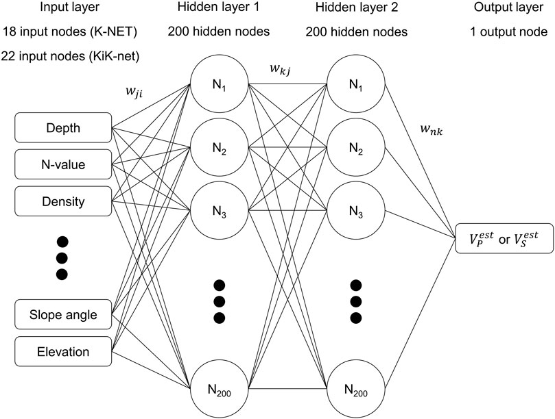
FIGURE 6. Architecture of the ANN-based model consists of an input layer, two hidden layers with 200 nodes (N), and an output layer. The weights between nodes (w) are illustrated.
Each node in an input layer receives an independent variable (e.g., the N-value). At each node, the value (
We applied a rectified linear unit (ReLU) to
Before training the model, the categorical variables (i.e., geology and soil/rock type) needed to be transformed into numerical variables. We mapped the variables into integers, which were then encoded in a binary format. This method is called binary encoding, which has been popularly utilized in applications (e.g., Jackson and Agrawal, 2019; Yousef et al., 2019). Here is an example using the soil/rock type in the K-NET dataset, which includes 12 unique features (i.e., 12 IDs). First, the length of the encoding vector was determined as
We applied the five-fold cross-validation (CV), which has been widely utilized in model evaluation (Berrar, 2019). This approach assesses the generalization ability of models and prevents overfitting. The five-fold CV divides the entire dataset randomly into five roughly equal folds. Then, the model uses four folds for training and the remaining one fold for testing (i.e., 80% for training and 20% for test dataset). We repeated for five times: i.e., we developed five ML models. The test results from these five experiments were aggregated to evaluate the general performance of the ML algorithm.
This study aims to train ML models using the data for some sites and evaluate the model performance using the data for new sites. Therefore, all data samples were split based on site locations and not on whole data samples. Each fold is allocated 20% of the total sites but may not be divided exactly. With our case as an example, the K-NET sites were divided into training and testing parts as follows: 797:199 (for four experiments), and 796:200 (for one experiment). For the KiK-net dataset, the VP data were divided into 541:136 (for two experiments) and 542:135 (for three experiments), and VS data were separated equally for all experiments: 540 for training and 135 for testing.
The three ML-based models developed in this study were evaluated for each test fold after training. Figure 7 presents the measured wave velocities (i.e.,
where
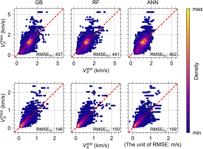
FIGURE 7. Measured velocity values (i.e.,
Figure 8 presents the measured wave velocities (i.e.,
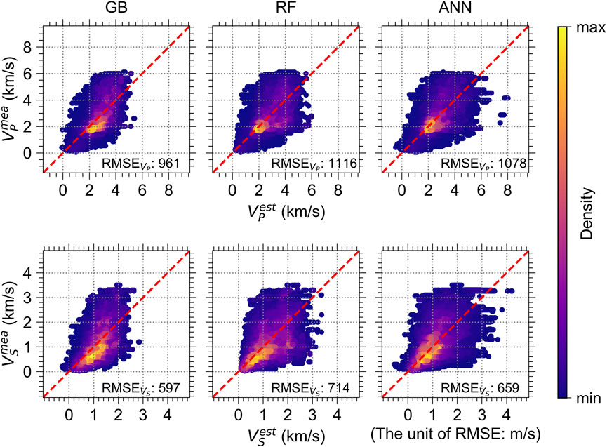
FIGURE 8. Measured velocity values (i.e.,
The RMSE depends on the study area and data features including the number of sites and velocities distribution. Many previous studies have utilized varying ranges of VS to make predictions for different geological regions, resulting in varied RMSEs. For example, Ataee et al. (2019) utilized uncorrected and corrected SPT-N with 88 boreholes to predict VS. The results using uncorrected SPT-N and VS under approximately 1,200 m/s presented that the RMSEs of the models ranged from 94.512 to 104.149 m/s. Those using corrected SPT-N and VS under approximately 600 m/s presented RMSEs ranging from 59.423 to 67.473 m/s. Ghorbani et al. (2012) utilized corrected SPT blow counts, and effective overburden stress to predict VS. They used 80 boreholes, where the VS ranges from 66 to 363 m/s. The RMSE of the prediction model is 37.2 m/s. Sun et al. (2013) used tip resistance, sleeve friction, pore pressure, and overburden effective stress to establish the correlation with VS. They utilized 17 sites, where the measured VS is under approximately 400 m/s. The RMSEs of the correlation forms are from 30.42 to 38.57 m/s. Furthermore, Dumke and Berndt (2019) used 38 types of variables (e.g., depth below seafloor, surface heat flow, and distance to nearest spreading ridge) to predict VP. They used 333 sites containing VP above 4,000 m/s, where the velocity range is not mentioned. The RMSEs vary approximately between 400 and 500 m/s depending on the considered variables. The RMSE presented in this paper may be reasonable, given that the prediction models were made and tested for the larger number of sites distributed throughout Japan, which includes various study areas and a wider range of velocities than other studies. However, discrepancies have been observed, especially for the KiK-net: VP dataset, implying that more region-specific depth-related variables may be needed to infer the velocity profiles better.
We further investigated the relationship between the measured and estimated velocities by employing the Regression Error Characteristic (REC) curve (Bi and Bennett, 2003). The REC curve depicts the relationship between the specified deviation tolerance on the x-axis, which is the error tolerance, and the y-axis for the proportion of data with prediction deviations smaller than the corresponding deviation. The resulting curve provides an estimation of the cumulative distribution function of the error. Furthermore, the REC curve quantifies the performance of the model by computing the area under the curve (AUC). A higher AUC value indicates better model performance. Figure 9 illustrates the REC curves for each model. The curves were individually computed for the five test folds from the five experiments and were then averaged to make a single curve. The AUC was subsequently calculated based on the single curve, representing the general performance of each model on the dataset. The results for K-NET and KiK-net, both at VP and VS, reveal that all AUCs are above 0.702 for the specified deviations ranging from 0 to 1.0. Notably, the GB-based model has the highest AUC across all cases, indicating its relatively strong predictive performance within the deviation range.
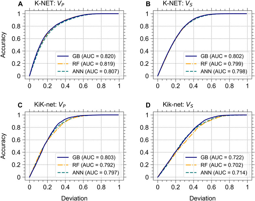
FIGURE 9. REC curves for individual models: (A) VP and (B) VS for K-NET, and (C) VP and (D) VS for KiK-net. Each curve represents the average accuracy across the five test folds from the five experiments (i.e., five derived ML models), with the specified deviation.
Figure 10 presents maps of RMSEs for the GB-based model for all the sites considered in this study, which were aggregated from five test folds from the five experiments (i.e., five derived ML models). Overall, the models for VP and VS of the K-NET sites (Figures 10A, B) indicate that almost 80% of the sites have RMSE values within the range of (0, 500] for VP, and almost 99% are within the same range for VS. In contrast, for KiK-net (Figures 10C, D), approximately 46% of the sites have RMSE values within the (500, 1,000] range for VP, and about 63% are within the (0, 500] range for VS. It can be noticed that the RMSE values larger than 1,000 m/s for the estimated VP values at the K-NET sites are concentrated in the area around 139 °E and 35.5 °N (Figure 10A). Furthermore, the RMSE values greater than 1,500 m/s and 1,000 m/s for the estimated VP and VS values, respectively, at the KiK-net sites are mainly clustered in the region around 137 °E and 35 °N (Figures 10C, D). The RMSEs for the KiK-net sites show a certain pattern along the east coast (from 140 to 142 °E and from 36 to 40 °N) (see Figure 10D). These observations imply that there could be factors that can affect the VS and VP values, other than those considered in this study.
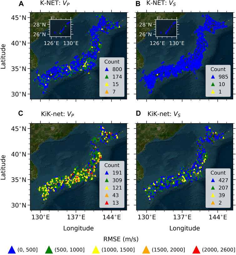
FIGURE 10. Maps for RMSE values of the GB-based model for (A) VP and (B) VS of all of the K-NET sites, and those for (C) VP and (D) VS of all of the KiK-net sites. The data for the sites were aggregated from five test folds of the five experiments (i.e., five derived ML models). The count numbers of the color-coded RMSE ranges are presented inside each of the panels.
Figure 11 shows examples of the wave velocity profiles predicted by the GB-based model compared with the measured profiles at the nine K-NET sites. The eight and one sample profiles were randomly selected from the VS RMSE bands of (0, 500] m/s and (500, 1,000] m/s, respectively, from the entire test folds from five experiments. The wave velocities predicted for the HKD024, FKO015, and KNG008 sites (Figures 11A–C, respectively) are in good agreement with the measured profiles when compared to the other illustration, producing RMSE values ≤186 m/s. In contrast, there are some discrepancies between the measured and predicted profiles at certain depth ranges for the rest of the sites. At GNM014, VP is overestimated at depths of up to 9 m (Figure 11D). At NGN025, the wave velocities are underestimated at depths greater than 13 m (Figure 11E). At EHM012, VP is underestimated at depths from 2 to 6 m (Figure 11F). There are also some discrepancies in the VP profiles at the YMT006, IBR009, and KGW008 sites (Figures 11G–I, respectively). In detail, the VP is consistently overestimated across the entire depth range at the YMT006 site (Figure 11G). At the IBR009 site, VP is underestimated up to a depth of 5 m (Figure 11H). Similarly, the KGW008 site demonstrates underestimation up to 3 m and overestimation at depths beyond 10 m (Figure 11I).
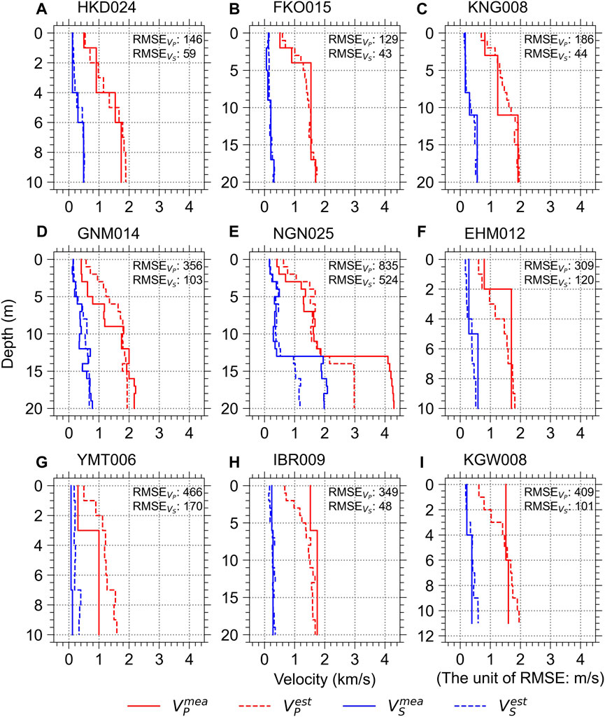
FIGURE 11. Measured wave velocity profiles (
Figure 12 presents examples of the wave velocity profiles estimated by the GB-based model compared with the measured profiles at the nine KiK-net sites. The six, two, and one sample profiles were randomly selected from the VS RMSE bands of (0, 500], (500, 1,000], and (1,500, 2000], respectively, from the entire test folds from five experiments. The estimated wave velocities for the HRSH15, KOCH11, IBRH12, and TCGH15 sites (Figures 12A–C, E, respectively) comparatively match well with the measured profiles, producing RMSE values ≤388 m/s. Some discrepancies are observed at specific depth ranges for the other sites. At IBRH07, the wave velocities are overestimated at depths from 51 m to 650 m and underestimated at depths from 651 m to 1,050 m (Figure 12D); however, the estimated wave velocities show relatively close agreement beyond 1,050 m. At SITH03, the velocities are overestimated almost throughout the depth (Figure 12F). At AICH12, the velocities are underestimated at depths greater than 49 m (Figure 12G). Overestimations are observed at the ISKH06 site for depths greater than 44 m (Figure 12H). For the YMTH08 site, velocities are overestimated for depths exceeding 18 m, while the VP is underestimated for depths up to 6 m (Figure 12I).
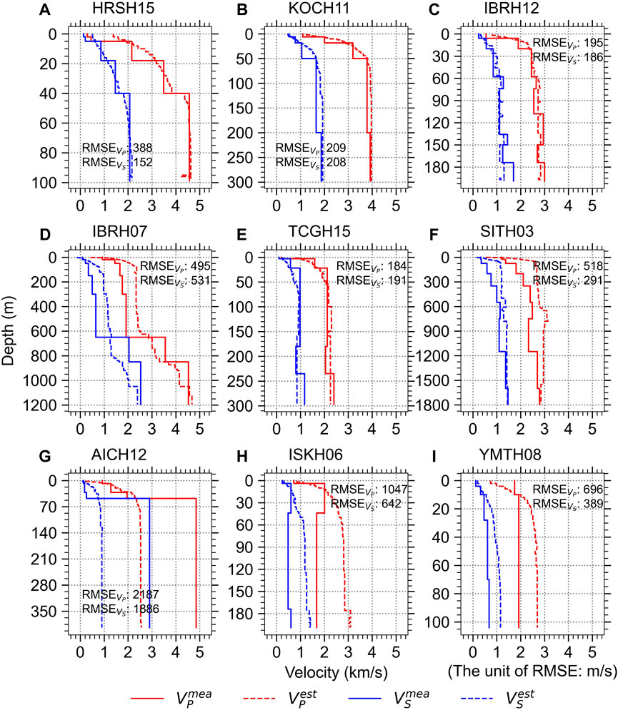
FIGURE 12. Measured wave velocity profiles (
Some discrepancies were observed in relation to a certain depth and profile patterns, as shown in Figure 11 and Figure 12. It is possible that the model could not well predict velocities for sites that have unusual profile patterns or for those that have not been frequently used when training or are not included in the training dataset. The model was trained to reduce the overall error for the entire sites used in training, so it might not well generalize the unseen patterns. As seen in the samples in Figure 11 and Figure 12, the model was trained to predict slower velocities near the ground surface and faster velocities at greater depths. Furthermore, model predicts velocities gradually increasing, and does not predict well the abrupt velocity changes (e.g., Figure 11E; Figure 12G). There are velocity reversals at depths greater than 44 m at ISKH06 (Figure 12H), and the VP values are unusually faster near the ground surface at YMTH08 (Figure 12I). It turned out that the model was not able to capture these profiles.
For the systematic evaluation of discrepancies between measured and estimated wave velocities, we computed the residuals for all the continuous variables as
where
Figure 13 shows the
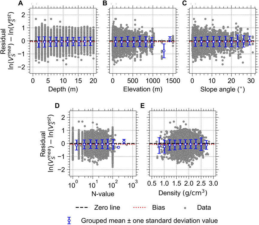
FIGURE 13. Residuals of the VS estimated by the GB-based model for the K-NET stations with respect to all the continuous variables: (A) depth; (B) elevation; (C) slope angle; (D) N-value; and (E) density. The data were aggregated from five test folds from the five experiments (i.e., five derived ML models).
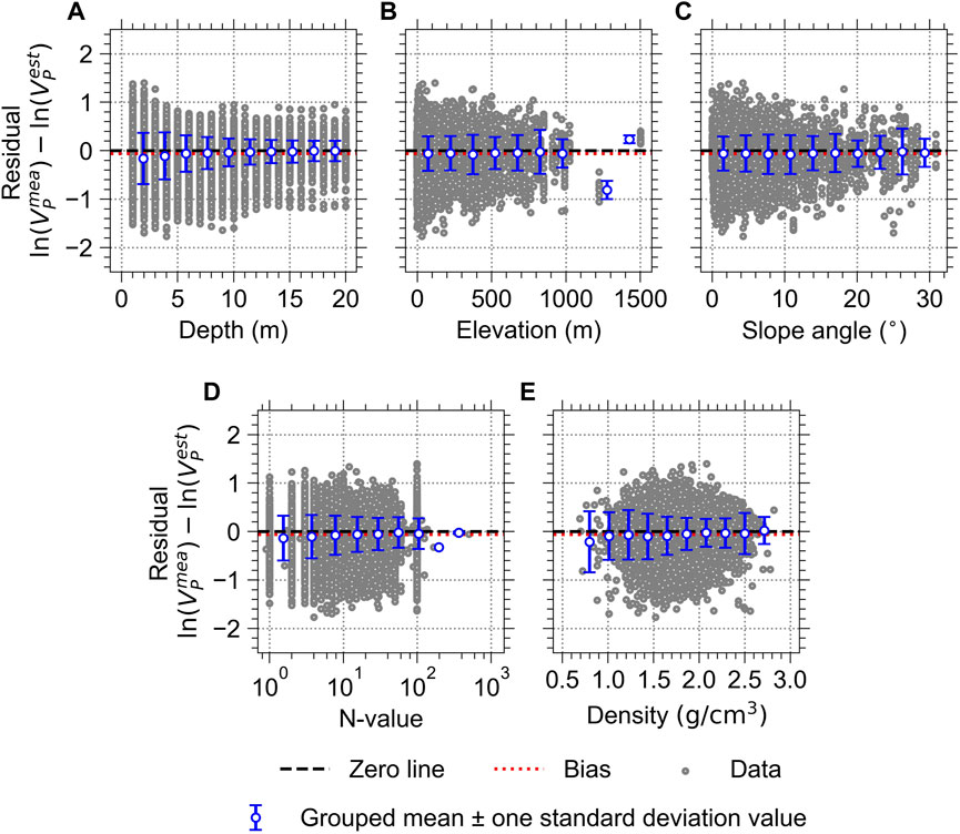
FIGURE 14. Residuals of the VP estimated by the GB-based model for the K-NET stations with respect to all the continuous variables: (A) depth; (B) elevation; (C) slope angle; (D) N-value; and (E) density. The data were aggregated from five test folds from the five experiments (i.e., five derived ML models).
We examined the contribution levels of the independent variables to the prediction accuracy of the best model, the GB-based model. The method is called variable importance (VI), which is computed as the sum of the decrease in error when a variable splits a tree node (e.g., a node split by an N-value
where
where
Figures 15A, B show the relative VIs for the K-NET independent variables for the GB-based models. The relative VI was computed by VI for each variable divided by the total VI for all variables. The VI was calculated on each test fold, and the VIs for all the five test folds were averaged. The VIs computed for binary codes were summed for the categorical variables. Three depth-dependent variables (i.e., depth, N-value, and density) have the highest VIs for both VP and VS models. The depth is ranked at the top for the VP model, whereas the N-value is ranked at the top for the VS model. Figures 15C, D present the relative VIs for the KiK-net dataset. The depth turned out to be the most critical variable for both VP and VS models. The effect of the site location is more significant for the KiK-net model than for the K-NET model. The slope angle and elevation have a certain influence on the models, whereas the soil/rock type and geology have the least influence. Although the influence of the geology turned out to be insignificant, the performance of the GB-based model was enhanced by including it. The RMSEs of the model were reduced from 615 m/s to 597 m/s for VS, and from 979 m/s to 961 m/s for VP, implying that it is also related to wave velocities at a deeper depth.
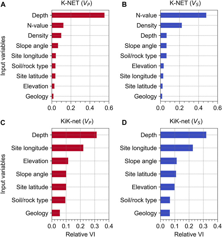
FIGURE 15. Relative variable importance (VI) for the GB-based models for (A) K-NET (VP), (B) K-NET (VS), (C) KiK-net (VP), and (D) KiK-net (VS). The variables are presented in an order of descending relative VI.
The confining pressure increases with depth, leading to an increase in the density, N-value, and wave velocities. Therefore, the depth and associated variables were determined to be most strongly correlated, as revealed by VI. The slope and elevation are related with shear stiffnesses, which eventually affect wave velocities. The site coordinates are relatively high VI, implying that they may be associated with site conditions that were not captured by other variables. The geology has the lowest VI, as it is for the ground surface. However, we included it in the model because of its certain effect in enhancing the predictive performance.
This paper presented three ML-based models (i.e., GB-, RF-, and ANN-based models) predicting VP and VS in Japan. We used borehole databases from the two seismograph networks, K-NET and KiK-net. We considered various factors such as depth, N-value, density, slope angle, elevation, geology, soil/rock type, and site coordinates. The number of trees was designated as 100 to train the RF- and GB-based models. We developed an ANN-based model with four layers, where each hidden layer included 200 nodes.
The models were trained and evaluated on the datasets using the five-fold cross-validation. The average RMSEs across all test folds showed that the GB-based model provided the best estimation among the other models for both K-NET and KiK-net sites. The RMSEs of the GB-based model for VS and VP of the K-NET sites were 146 and 437 m/s, respectively, and those of the KiK-net sites were 597 and 961 m/s, respectively, while those of the other models ranging from 150 to 462 m/s for K-NET and from 659 to 1,116 m/s for KiK-net. Furthermore, the REC curve indicated that the GB-based model revealed relatively high performance within the deviation range. We also validated the GB-based model by checking the residuals between the measured and estimated wave velocities with respect to various variables. The variable importance of the model for K-NET indicated that depth, N-value, and density were the essential variables in predicting the VP and VS of the K-NET sites. Note that we used the unnormalized N-values for the K-NET sites, which might lower the prediction capability. For KiK-net sites, depth was the most influential variable. The site longitude also had a high relative variable importance value, indicating the roles of factors other than those considered in this study. The geology has the smallest VI values, as shown in Figure 15. However, it turned out that including the geology can improve the model performance, decreasing the RMSE values. In addition, we consider that including latitude and longitude is necessary because these improved prediction performances of the models, capturing the effects that were not captured by other variables.
This paper proposed a model for predicting wave velocities based on various factors, which can be used for site exploration in various fields, including rock engineering and petroleum engineering. The key findings of this study highlight that common machine learning algorithms can reasonably predict the wave velocity profiles across the region of Japan as an example. The results from cross-validation present the general performances of models on the dataset and site-specific performances specifically for the GB-based model. The study reveals the importance of input variables contributing to predicting accuracy. Moreover, it suggests that considering more region-specific variables including site coordinates can assist the models in interpreting complicated relationships.
As for the limitations of this study, the models are limited by their reliance on borehole databases exclusively obtained from specific seismograph networks in Japan. This approach may present a bias towards the conditions within these networks. Consequently, predictive performance could be constrained when extending the applications to regions with different geological attributes. In this context, ensuring the consistency of the environmental and experimental conditions, and the employed measured data is crucial to guarantee the validity of results beyond the area considered in this study. Additionally, even though the various variables were included, an incomplete representation remains for specific regions. This implies the presence of intricate geological properties that necessitate analysis to understand their influence on the prediction of wave velocities in a particular area. Furthermore, the study reveals that incorporating site coordinates can influence predictive performance. Nevertheless, the specific contributions of these variables to predictive performance concerning geological characteristics remain subject to consideration. While this study confirmed that the most commonly used machine-learning techniques could be successfully applied for predicting wave velocities, exploring more advanced techniques and investigating additional factors in the future will enhance the prediction performance.
Publicly available datasets were analyzed in this study. This data can be found here: https://www.kyoshin.bosai.go.jp/, Strong-motion Seismograph Networks (K-NET, KiK-net).
JK: Conceptualization, Data curation, Formal Analysis, Methodology, Validation, Visualization, Writing–original draft, Writing–review and editing. J-DK: Conceptualization, Data curation, Formal Analysis, Writing–original draft. BK: Conceptualization, Formal Analysis, Funding acquisition, Project administration, Supervision, Writing–original draft, Writing–review and editing.
This work was supported by KOREA HYDRO & NUCLEAR POWER CO., LTD (No. 2022-Tech-03) and the Korea Agency for Infrastructure Technology Advancement (KAIA) grant funded by the Ministry of Land, Infrastructure, and Transport (Grant 21CATAP-C164148-01). The funder was not involved in the study design, collection, analysis, interpretation of data, the writing of this article, or the decision to submit it for publication. The opinions, findings, and conclusions or recommendations expressed in this article are solely those of the authors and do not represent those of the funders.
We are indebted to the National Research Institute for Earth Science and Disaster Resilience (NIED), Japan, for making the resources of K-NET and KiK-net seismographs publicly available.
The authors declare that the research was conducted in the absence of any commercial or financial relationships that could be construed as a potential conflict of interest.
All claims expressed in this article are solely those of the authors and do not necessarily represent those of their affiliated organizations, or those of the publisher, the editors and the reviewers. Any product that may be evaluated in this article, or claim that may be made by its manufacturer, is not guaranteed or endorsed by the publisher.
The Supplementary Material for this article can be found online at: https://www.frontiersin.org/articles/10.3389/feart.2023.1267386/full#supplementary-material
Abadi, M., Agarwal, A., Barham, P., Brevdo, E., Chen, Z., Citro, C., et al. (2016). Tensorflow: large-scale machine learning on heterogeneous distributed systems. arXiv preprint arXiv:1603.04467.
Akin, M. K., Kramer, S. L., and Topal, T. (2011). Empirical correlations of shear wave velocity (Vs) and penetration resistance (SPT-N) for different soils in an earthquake-prone area (Erbaa-Turkey). Eng. Geol. 119 (1-2), 1–17. doi:10.1016/j.enggeo.2011.01.007
Ameen, M. S., Smart, B. G., Somerville, J. M., Hammilton, S., and Naji, N. A. (2009). Predicting rock mechanical properties of carbonates from wireline logs (A case study: arab-D reservoir, ghawar field, Saudi arabia). Mar. Petroleum Geol. 26 (4), 430–444. doi:10.1016/j.marpetgeo.2009.01.017
Andrus, R. D., Piratheepan, P., Ellis, B. S., Zhang, J., and Juang, C. H. (2004). Comparing liquefaction evaluation methods using penetration-VS relationships. Soil Dyn. Earthq. Eng. 24 (9-10), 713–721. doi:10.1016/j.soildyn.2004.06.001
Anemangely, M., Ramezanzadeh, A., Amiri, H., and Hoseinpour, S.-A. (2019). Machine learning technique for the prediction of shear wave velocity using petrophysical logs. J. Petroleum Sci. Eng. 174, 306–327. doi:10.1016/j.petrol.2018.11.032
Ataee, O., Moghaddas, N. H., and Lashkaripour, G. R. (2019). Estimating shear wave velocity of soil using standard penetration test (SPT) blow counts in Mashhad city. J. Earth Syst. Sci. 128 (3), 1–25. doi:10.1007/s12040-019-1077-x
Bajaj, K., and Anbazhagan, P. (2019). Seismic site classification and correlation between VS and SPT-N for deep soil sites in Indo-Gangetic Basin. J. Appl. Geophys. 163, 55–72. doi:10.1016/j.jappgeo.2019.02.011
Berrar, D. (2019). Cross-validation. Encycl. Bioinforma. Comput. Biol. 1, 542–545. doi:10.1016/B978-0-12-809633-8.20349-X
Bi, J., and Bennett, K. P. (2003). “Regression error characteristic curves,” in Proceedings of the 20th international conference on machine learning (ICML-03)), Washington, DC USA, August 21 - 24, 2003, 43–50.
Boob, D., Dey, S. S., and Lan, G. (2020). Complexity of training relu neural network. Discrete Optim. 2020, 100620. doi:10.1016/j.disopt.2020.100620
Chang, C., Zoback, M. D., and Khaksar, A. (2006). Empirical relations between rock strength and physical properties in sedimentary rocks. J. Petroleum Sci. Eng. 51 (3-4), 223–237. doi:10.1016/j.petrol.2006.01.003
Czajkowski, M., and Kretowski, M. (2019). Decision tree underfitting in mining of gene expression data. An evolutionary multi-test tree approach. Expert Syst. Appl. 137, 392–404. doi:10.1016/j.eswa.2019.07.019
Deng, C., Pan, H., Fang, S., Konaté, A. A., and Qin, R. (2017). Support vector machine as an alternative method for lithology classification of crystalline rocks. J. Geophys. Eng. 14 (2), 341–349. doi:10.1088/1742-2140/aa5b5b
Ding, P., Wang, D., Di, G., and Li, X. (2019). Investigation of the effects of fracture orientation and saturation on the Vp/Vs ratio and their implications. Rock Mech. Rock Eng. 52 (9), 3293–3304. doi:10.1007/s00603-019-01770-3
Dumke, I., and Berndt, C. (2019). Prediction of seismic P-wave velocity using machine learning. Solid earth. 10 (6), 1989–2000. doi:10.5194/se-10-1989-2019
Eberli, G. P., Baechle, G. T., Anselmetti, F. S., and Incze, M. L. (2003). Factors controlling elastic properties in carbonate sediments and rocks. Lead. Edge 22 (7), 654–660. doi:10.1190/1.1599691
Fiorentino, G., Quaranta, G., Mylonakis, G., Lavorato, D., Pagliaroli, A., Carlucci, G., et al. (2019). Seismic reassessment of the leaning tower of pisa: dynamic monitoring, site response, and SSI. Earthq. Spectra 35 (2), 703–736. doi:10.1193/021518EQS037M
Friedman, J. H. (2001). Greedy function approximation: a gradient boosting machine. Ann. Statistics 29, 1189–1232. doi:10.1214/aos/1013203451
Friedman, J. H. (2002). Stochastic gradient boosting. Comput. Statistics Data Analysis 38 (4), 367–378. doi:10.1016/S0167-9473(01)00065-2
Geological Survey of Japan (2015). Seamless digital geological map of Japan 1: 200,000. Japan: National Institute of Advanced Industrial Science and Technology.
Geurts, P., Irrthum, A., and Wehenkel, L. (2009). Supervised learning with decision tree-based methods in computational and systems biology. Mol. Biosyst. 5 (12), 1593–1605. doi:10.1039/B907946G
Ghorbani, A., Jafarian, Y., and Maghsoudi, M. S. (2012). Estimating shear wave velocity of soil deposits using polynomial neural networks: application to liquefaction. Comput. Geosciences 44, 86–94. doi:10.1016/j.cageo.2012.03.002
Harmon, J., Hashash, Y. M., Stewart, J. P., Rathje, E. M., Campbell, K. W., Silva, W. J., et al. (2019). Site amplification functions for central and eastern north America–Part II: modular simulation-based models. Earthq. Spectra 35 (2), 815–847. doi:10.1193/091117EQS179M
Hasancebi, N., and Ulusay, R. (2007). Empirical correlations between shear wave velocity and penetration resistance for ground shaking assessments. Bull. Eng. Geol. Environ. 66 (2), 203–213. doi:10.1007/s10064-006-0063-0
Heath, D. C., Wald, D. J., Worden, C. B., Thompson, E. M., and Smoczyk, G. M. (2020). A global hybrid VS30 map with a topographic slope–based default and regional map insets. Earthq. Spectra 36 (3), 1570–1584. doi:10.1177/8755293020911137
Jackson, E., and Agrawal, R. (2019). “Performance Evaluation of different feature Encoding schemes on cybersecurity logs,” in 2019 SoutheastCon., 11-14 April 2019.
Jamshidi, A., Zamanian, H., and Sahamieh, R. Z. (2018). The effect of density and porosity on the correlation between uniaxial compressive strength and P-wave velocity. Rock Mech. Rock Eng. 51 (4), 1279–1286. doi:10.1007/s00603-017-1379-8
Jena, R., Pradhan, B., Almazroui, M., Assiri, M., and Park, H.-J. (2023). Earthquake-induced liquefaction hazard mapping at national-scale in Australia using deep learning techniques. Geosci. Front. 14 (1), 101460.doi:10.1016/j.gsf.2022.101460
Jun, M.-J. (2021). A comparison of a gradient boosting decision tree, random forests, and artificial neural networks to model urban land use changes: the case of the seoul metropolitan area. Int. J. Geogr. Inf. Sci. 35 (11), 2149–2167. doi:10.1080/13658816.2021.1887490
Karthikeyan, J., and Samui, P. (2014). Application of statistical learning algorithms for prediction of liquefaction susceptibility of soil based on shear wave velocity. Geomatics, Nat. Hazards Risk 5 (1), 7–25. doi:10.1080/19475705.2012.757252
Kim, B. (2019). Mapping of ground motion amplifications for the fraser river delta in greater vancouver, Canada. Earthq. Eng. Eng. Vib. 18 (4), 703–717. doi:10.1007/s11803-019-0531-8
Kim, S., Hwang, Y., Seo, H., and Kim, B. (2020). Ground motion amplification models for Japan using machine learning techniques. Soil Dyn. Earthq. Eng. 132, 106095. doi:10.1016/j.soildyn.2020.106095
Kottke, A. R., Hashash, Y., Stewart, J. P., Moss, C. J., Nikolaou, S., Rathje, E. M., et al. (2012). “Development of geologic site classes for seismic site amplification for central and eastern North America,” in 15th World Conf. on Earthquake Engineering, Lisbon, Portugal, September 24 to September 28, 2012.
Krauss, C., Do, X. A., and Huck, N. (2017). Deep neural networks, gradient-boosted trees, random forests: statistical arbitrage on the S&P 500. Eur. J. Operational Res. 259 (2), 689–702. doi:10.1016/j.ejor.2016.10.031
Kwak, D. Y., Brandenberg, S. J., Mikami, A., and Stewart, J. P. (2015). Prediction equations for estimating shear-wave velocity from combined geotechnical and geomorphic indexes based on Japanese data set. Bull. Seismol. Soc. Am. 105 (4), 1919–1930. doi:10.1785/0120140326
Kwok, O. L. A., Stewart, J. P., Kwak, D. Y., and Sun, P.-L. (2018). Taiwan-specific model for VS30 prediction considering between-proxy correlations. Earthq. Spectra 34 (4), 1973–1993. doi:10.1193/061217EQS113M
National Research Institute for Earth Science and Disaster Resilience (2019). NIED K-NET, KiK-net, national research Institute for Earth science and disaster resilience. Natl. Res. Inst. Earth Sci. Disaster Resil. 2019. doi:10.17598/NIED.0004
Ohta, Y., and Goto, N. (1978). Empirical shear wave velocity equations in terms of characteristic soil indexes. Earthq. Eng. Struct. Dyn. 6 (2), 167–187. doi:10.1002/eqe.4290060205
Panza, E., Agosta, F., Rustichelli, A., Vinciguerra, S., Ougier-Simonin, A., Dobbs, M., et al. (2019). Meso-to-microscale fracture porosity in tight limestones, results of an integrated field and laboratory study. Mar. Petroleum Geol. 103, 581–595. doi:10.1016/j.marpetgeo.2019.01.043
Pappalardo, G. (2015). Correlation between P-wave velocity and physical–mechanical properties of intensely jointed dolostones, Peloritani mounts, NE Sicily. Rock Mech. Rock Eng. 48 (4), 1711–1721. doi:10.1007/s00603-014-0607-8
Parker, G. A., Harmon, J. A., Stewart, J. P., Hashash, Y. M., Kottke, A. R., Rathje, E. M., et al. (2017). Proxy-based VS30 estimation in central and eastern North America. Bull. Seismol. Soc. Am. 107 (1), 117–131. doi:10.1785/0120160101
Paul, S., Ali, M., and Chatterjee, R. (2018). Prediction of compressional wave velocity using regression and neural network modeling and estimation of stress orientation in Bokaro Coalfield, India. Pure Appl. Geophys. 175 (1), 375–388. doi:10.1007/s00024-017-1672-1
Pedregosa, F., Varoquaux, G., Gramfort, A., Michel, V., Thirion, B., Grisel, O., et al. (2011). Scikit-learn: machine learning in Python. J. Mach. Learn. Res. 12, 2825–2830.
Pickett, G. R. (1963). Acoustic character logs and their applications in formation evaluation. J. Petroleum Technol. 15 (6), 659–667. doi:10.2118/452-PA
Rahimi, S., Wood, C. M., and Wotherspoon, L. M. (2020). Influence of soil aging on SPT-Vs correlation and seismic site classification. Eng. Geol. 272, 105653. doi:10.1016/j.enggeo.2020.105653
Rahman, T., and Sarkar, K. (2021). Lithological control on the estimation of uniaxial compressive strength by the P-wave velocity using supervised and unsupervised learning. Rock Mech. Rock Eng. 54, 3175–3191. doi:10.1007/s00603-021-02445-8
Roy, D. G., Singh, T., Kodikara, J., and Das, R. (2017). Effect of water saturation on the fracture and mechanical properties of sedimentary rocks. Rock Mech. Rock Eng. 50 (10), 2585–2600. doi:10.1007/s00603-017-1253-8
Samui, P., Kim, D., and Sitharam, T. (2011). Support vector machine for evaluating seismic-liquefaction potential using shear wave velocity. J. Appl. Geophys. 73 (1), 8–15. doi:10.1016/j.jappgeo.2010.10.005
Seo, H., Kim, J., and Kim, B. (2022). Machine-learning-based surface ground-motion prediction models for South Korea with low-to-moderate seismicity. Bull. Seismol. Soc. Am. 112 (3), 1549–1564. doi:10.1785/0120210244
Si, W., Di, B., Wei, J., and Li, Q. (2016). Experimental study of water saturation effect on acoustic velocity of sandstones. J. Nat. Gas Sci. Eng. 33, 37–43. doi:10.1016/j.jngse.2016.05.002
Sil, A., and Haloi, J. (2017). Empirical correlations with standard penetration test (SPT)-N for estimating shear wave velocity applicable to any region. Int. J. Geosynth. Ground Eng. 3 (3), 1–13. doi:10.1007/s40891-017-0099-1
Singh, S., and Kanli, A. I. (2016). Estimating shear wave velocities in oil fields: a neural network approach. Geosciences J. 20 (2), 221–228. doi:10.1007/s12303-015-0036-z
Sousa, L. M., del Río, L. M. S., Calleja, L., de Argandona, V. G. R., and Rey, A. R. (2005). Influence of microfractures and porosity on the physico-mechanical properties and weathering of ornamental granites. Eng. Geol. 77 (1-2), 153–168. doi:10.1016/j.enggeo.2004.10.001
Sun, C.-G., Cho, C.-S., Son, M., and Shin, J. S. (2013). Correlations between shear wave velocity and in-situ penetration test results for Korean soil deposits. Pure Appl. Geophys. 170 (3), 271–281. doi:10.1007/s00024-012-0516-2
Tsai, C.-C., Kishida, T., and Kuo, C.-H. (2019). Unified correlation between SPT–N and shear wave velocity for a wide range of soil types considering strain-dependent behavior. Soil Dyn. Earthq. Eng. 126, 105783. doi:10.1016/j.soildyn.2019.105783
Wang, P., and Peng, S. (2019). On a new method of estimating shear wave velocity from conventional well logs. J. Petroleum Sci. Eng. 180, 105–123. doi:10.1016/j.petrol.2019.05.033
Xiao, S., Zhang, J., Ye, J., and Zheng, J. (2021). Establishing region-specific N–Vs relationships through hierarchical Bayesian modeling. Eng. Geol. 287, 106105. doi:10.1016/j.enggeo.2021.106105
Yasar, E., and Erdogan, Y. (2004). Correlating sound velocity with the density, compressive strength and Young's modulus of carbonate rocks. Int. J. Rock Mech. Min. Sci. 41 (5), 871–875. doi:10.1016/j.ijrmms.2004.01.012
Yousef, W. A., Ibrahime, O. M., Madbouly, T. M., and Mahmoud, M. A. (2019). Learning meters of Arabic and English poems with recurrent neural networks: A step forward for language understanding and synthesis. arXiv preprint arXiv:1905.05700.
Keywords: shear wave velocity, compression wave velocity, machine learning, gradient boosting, random forest, artificial neural network, cross-validation
Citation: Kim J, Kang J-D and Kim B (2023) Machine-learning models to predict P- and S-wave velocity profiles for Japan as an example. Front. Earth Sci. 11:1267386. doi: 10.3389/feart.2023.1267386
Received: 26 July 2023; Accepted: 26 September 2023;
Published: 16 October 2023.
Edited by:
Biswajeet Pradhan, University of Technology Sydney, AustraliaReviewed by:
Pijush Samui, National Institute of Technology Patna, IndiaCopyright © 2023 Kim, Kang and Kim. This is an open-access article distributed under the terms of the Creative Commons Attribution License (CC BY). The use, distribution or reproduction in other forums is permitted, provided the original author(s) and the copyright owner(s) are credited and that the original publication in this journal is cited, in accordance with accepted academic practice. No use, distribution or reproduction is permitted which does not comply with these terms.
*Correspondence: Byungmin Kim, Ynl1bmdtaW4ua2ltQHVuaXN0LmFjLmty
Disclaimer: All claims expressed in this article are solely those of the authors and do not necessarily represent those of their affiliated organizations, or those of the publisher, the editors and the reviewers. Any product that may be evaluated in this article or claim that may be made by its manufacturer is not guaranteed or endorsed by the publisher.
Research integrity at Frontiers

Learn more about the work of our research integrity team to safeguard the quality of each article we publish.