 Srđan Kostić
 Milan Stojković
94% of researchers rate our articles as excellent or good
Learn more about the work of our research integrity team to safeguard the quality of each article we publish.
Find out more
ORIGINAL RESEARCH article
Front. Earth Sci., 08 November 2023
Sec. Geohazards and Georisks
Volume 11 - 2023 | https://doi.org/10.3389/feart.2023.1267225
This article is part of the Research TopicContemporary Characterization and Modeling of Earth Processes: A Multidisciplinary ApproachView all 4 articles
In the present paper we examine the effect of the noise in river level oscillation on the landslide dynamics. The analysis is conducted in several phases. In the first phase, we analyze the multi-annual level oscillation of the Kolubara and the Ibar river (Serbia). Based on the observed dataset, we suggest a deterministic model for the river level oscillation with the additional contribution of the noise part, which we confirm to have the properties of colored noise. In the second phase of the research, we introduce the influence of the river-level oscillation, with the included effect of colored noise in the spring-block delay model of landslide dynamics. Results of the research indicate conditions under which the effect of river noise has both stabilizing and destabilizing effects on the landslide dynamics. The effect of noise intensity D and correlation time ε is systematically analyzed in interaction with delayed interaction, spring stiffness and friction parameters. It is determined that the landslide dynamics is sensitive to the change of noise intensity and that the increase of noise intensity leads to onset of unstable landslide dynamics. On the other hand, results obtained indicate that the examined model of landslide dynamics is rather robust towards the change of correlation time ε. Interaction of this parameter and some of the friction parameters leads to stabilization of landslide dynamics, which confirms the importance of the influence of the noise color in river level oscillations on the landslide dynamics.
The main external triggering factors of a slope instability (e.g., landslides) commonly depend on the corresponding surroundings of the potentially unstable feature itself. For example, in active seismic regions, (re)activation of landslides often occurs due to the dynamic impact; in wet and rainy areas, the rainfall is the primary contributing factor of the slope instability. In case when slope actually represents a river bank, activation of slope instability is caused by the regime of river level oscillations. In any of these cases, it is assumed that the geological composition and slope geometry provide initial conditions for the possible occurrence of landslides, i.e., existence of weak rock masses, with impermeable bedrock at a reasonable depth and steep inclination of the slope. Depending on the particular values of these slope properties, initial conditions could be close or far from the instability point. If initial conditions are far from the instability point, then the impact of any of the aforementioned external triggering factors should be strong enough to push the slope over the stability limit. In such cases, the strength of the external factor could be measured by the intensity, frequency or duration of the event. On the other hand, if initial conditions of the slope are close to instability point, then even a small external force could be sufficient to trigger the landslide. Both from the theoretical and practical viewpoint, this case is more interesting, since small disturbing external effect is ubiquitous and ever-present, so one may ask two questions: 1) what is the minimum threshold of this external force required to activate the instability? 2) in what state is the slope most sensitive to this small external effect? In the present paper, we try to provide answers to these questions for the following scenario: influence of the noise in river level oscillations on the occurrence of unstable landslide dynamics. In accordance with this main topic of the paper, we postulate the starting hypotheses of our research: i) river level oscillations could induce slope instability; ii) noise is the main constituent part of the river level oscillations; iii) type of noise and noise properties have significant effect on landslide dynamics.
Regarding the first starting hypothesis, there are many previous studies that confirmed the river level oscillation as the main contributing factor of landslide triggering. In particular, Abam (1993) determined several main mechanisms of the riverbank failures: rotational, translational, overhang/toppling and flow mechanism, which commonly occur at the early stages of lowering of channel water level. Dapporto et al. (2001) determined two dominant mechanisms of riverbank failure, namely, slab-type and alcove-shaped sliding failures, depending on different river stages. Ujvari et al. (2009) proposed a model for slope failure evolution based on the investigation of the Danube riverbank stability at Dunaszekcso. In their work they compared geodetic datasets and field observations with the timing of rainfall and water level changes of the Danube and concluded that perched water table, among others, was responsible for landslide triggering. Duong et al. (2014) examined the variations of the riverbank stability with the river level fluctuations, for the case study of the Red River of Hanoi (Vietnam). Based on the research conducted, they concluded that the pore water pressure and the rate of the river level change are the most important factors affecting the riverbank stability when hydraulic conductivity of the soil is greater than 10−6 m/s. Liang et al. (2015) examined the influence and sensitivity of river level fluctuations and climatic factors on riverbank stability. They determined that river level fluctuations dominate riverbank collapse in the Lower River Murray (South Australia). Chen et al. (2017) investigated the influences of drawdown rate of river stage, initial water elevation, and riverbank slope angle on riverbank stability due to the fall of river water level. As a result, they suggested a model for riverbank stability which includes the integral effect of all forces acting upon the failure plane and tension crack. Duong and Do (2019) investigated the influence of the fluctuation of the river water level on the shape of the riverbank cantilever failure, i.e., the low-rate rise of the river level could lead to a mass failure, while the high-rate rise of river level may lead to the overhanging riverbank failure. Mentes (2019) examined the relationship between riverbank stability and hydrological processes using in situ measurement data. As a result, an early warning system was developed, combining the effect of the groundwater level and river level fluctuations with the displacements measured by borehole tiltmeters.
As could be seen from the aforementioned, the impact of the river level fluctuations on the riverbank stability is well studied and could be considered as expected. Nevertheless, in the present paper, we investigate the conditions of the existing landslides along the riverbank for which the effect of the noise in the river level fluctuations is significant. As far as we are aware, this has not been examined before. Motivation for this research topic comes from two main sources. First, we have previously shown that noise could have significant impact to the dynamics of certain dynamical systems, under the condition that such systems are in “critical” state. For instance, we previously showed that the background-colored noise with low correlation time could trigger different dynamical regimes of seismogenic fault motion, namely, steady stationary state, aseismic creep and seismic fault motion (Kostić et al., 2020). On the other hand, we also showed that noise could have “stabilizing'” effect on the system’s dynamics: the increase of the intensity of the random background noise could lead to stabilization of the landslide dynamics (Kostić et al., 2023). Secondly, some previous studies indicated the existence of noise in river flow fluctuations. In particular, Vračar and Mijić (2011) investigated hydroacoustic noise in the Danube, the Sava and the Tisza River. Results of their research indicated that noise spectra are characterized by wide maximums at frequencies between 20 and 30 Hz, while spectral level of noise changes in wide limits. Tu et al. (2023) analyzed timescale-dependence of the noise color in streamflow across the US hydrography, using streamflow time series from 7,504 gauges. As a result, they found that daily and annual flows are dominated by red and white spectra, respectively. In contrast to these previous studies, in present paper we focus on the river level fluctuations rather than flow fluctuations, since the effect of river flow on the riverbank stability (which also includes the erosion) is not studied in current research.
It should be emphasized that in present study we start from the main assumption that landslide already exists along the riverbank, but it is in a creep regime, i.e., slope is moving constantly, but with very low velocity and, consequently, small constant displacements. Therefore, we do not analyze conditions for the occurrence of landslide displacement, but the conditions for the occurrence of unstable landslide dynamics. Such scenario is very common in real conditions: for example, the whole right bank of the Danube River, from Belgrade (Serbia) to the HPP Iron Gate 2 is at many points under the impact of long-lasting creeping landslides, whose activity is for many decades controlled by the regime of HPP Iron Gate 1 and Iron Gate 2.
The presented research is structured as follows. Firstly, we analyze the river level fluctuations for two case studies: the Kolubara River (Beli Brod hydrological station) and the Ibar River (Lopatnica Lakat hydrological station). For these examples, we derive deterministic oscillatory model, with the added noise effect. Secondly, we confirm the existence of colored noise in river level oscillations. In the third part of the research, we incorporate the effect of the colored noise in the previously suggested general model of landslide dynamics. Dynamics of such model is further examined, and three main points are addressed: 1) the conditions of the existing landslide along the riverbank for which the effect of the colored noise is relevant, 2) the nature of the effect of the colored noise, and 3) the size of the colored noise which is relevant for the significant change in landslide dynamics.
In the first phase of the research, we examined previously recorded river water levels. In general, the river water levels display considerable variations both annually and over long-term periods. Consequently, a reliable model for simulating water levels, which accounts for seasonal and monthly changes, is suggested. This model consists of two parts: seasonal
where
Initially, the seasonal component is deduced by utilizing the LOWESS (Locally Weighted Scatterplot Smoothing) regression method (Kostić et al., 2019), with the aim of filtering out noise (residual part) from the observed water levels. Subsequently, the filtered water levels are represented as a timely dependent function comprising stationary signals by the usage of spectral analysis (Stojković et al., 2017). The following equation is employed to mimic the seasonal component of the water level time series:
where
Regarding the procedure of noise separation from the main part of the time series - in the present paper, we examine finite dataset comprised of discrete measurements of river level. In order to simulate the continuous river level oscillations, we firstly develop a deterministic model of river level oscillations, as a limited combination of sine and cosine waves, where residuals are treated as noise.
In the second phase of the research, we introduced the river level variations, with the included noise into the previously suggested landslide model. Local dynamics of such model is then examined numerically using Runge-Kutta fourth order method. In all examined cases, initial conditions are set near the equilibrium state: x1=x2=1.001, y1=y2=0.002, z1=z2=0.001, θ=0.001.
This study focuses on the analysis of monthly water levels in the Kolubara and Ibar rivers (Figure 1). The Ibar River, a major tributary of the Western Morava River, merges with it near Kraljevo in Central Serbia. With a length of approximately 272 km and drainage area of 13.059 km2, the Ibar is among Serbia’s longest rivers. Conversely, the Kolubara River, a key tributary of the Sava River, stretches over 123 km and drains 3,600 km2. Originating from the western region of Serbia, the Kolubara flows through the Valjevo valley and passes the Kolubara coal basin, a crucial energy source in Serbia, as it moves northward.
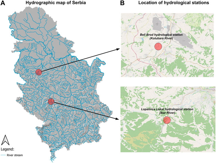
FIGURE 1. Hydrological map of Serbia (A) with location of hydrological stations (B).
Lopatnica Lakat and Beli Brod hydrological stations, located on the Ibar and Kolubara rivers respectively, are selected for analysis as they exhibit minimal anthropogenic impacts on the hydrological regime, such as flow regulation from upstream dams. Hydrological data are obtained from the Water Management Study of Serbia (WMSS, 2010), which includes records up to 2007. Table 1 provides the most important physical characteristics and available recording periods of hydrological stations analysed.

TABLE 1. The main characteristic of Beli Brod (Kolubara River) and Lopatnica Lakat (Ibar River) hydrological stations.
Water levels are smoothed using the local-regression LOESS method to extract the seasonal component (
Once the seasonal component is extracted, its characteristics are estimated in the frequency domain using Spectral analysis. The significant seasonal harmonics are identified for both hydrological stations (Beli Brod at the Kolubara River and Lopatnica Lakat at the Ibar River) using the Relative Cumulative Periodogram. For this purpose, a significant level of 95% is selected as it represents a substantial part of seasonal variance. The main properties of statistically significant harmonics for a 12-month time window filtering are provided in Table 2 for hydrological station considered.
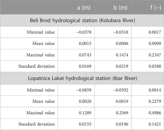
TABLE 2. Statistical properties of seasonal components at Beli Brod (Kolubara River) and Lopatnica Lakat (Ibar River) hydrological stations:
It is important to highlight that the most significant periodic component for both stations expectedly has an oscillation period of 12 months. It accounts for 8.2% and 4.6% of the total variance of the seasonal component for Beli Brod and Lopatnica Lakat hydrological stations, respectively. Additionally, the subsequent five significant harmonics cumulatively explain 22.6% of the variance in the time series of Beli Brod station (Kolubara River). At the Lopatnica Lakat site of the Ibar River, the next five harmonics account for 10.0% of the overall seasonal variation.
The remaining part of the time series modeling (Eq. 1) represents residuals (
The seasonal components of the water levels for the Kolubara (Beli Brod) and Ibar River (Lopatnica Lakat) are modeled and depicted in Figure 2. It considers harmonics that reach a significant level of 95% for three smoothing/filtering window lengths: 12, 30 and 6 months. Furthermore, Figure 2B displays the residual of the modeled seasonal component for both stations and filtering window lengths considered.
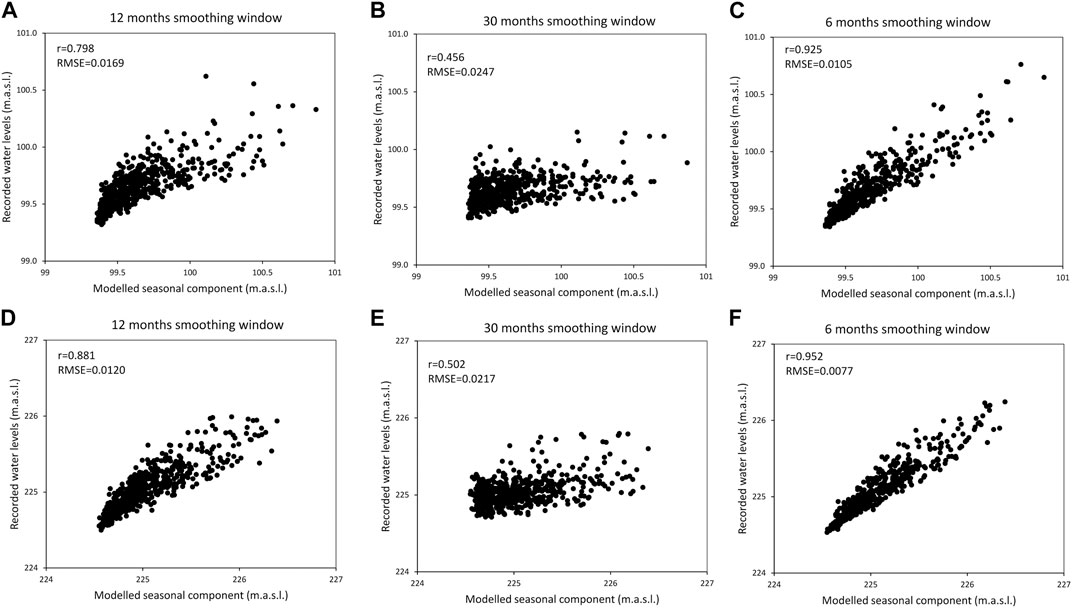
FIGURE 2. Upper row: recorded water levels
The results obtained suggest that the minimal seasonal component is achieved during the autumn months, specifically in the ninth and eighth months for the Kolubara and Ibar rivers, respectively. The water levels peak in spring, with the Ibar river recording the highest levels in the third month, while the Kolubara water levels peak in the fourth month. These variations in the seasonal water level components signify differences in the hydro-climatic regimes and morphological factors.
The modeled seasonal component and water levels for hydrological stations considered are also illustrated in Figure 2. The given figures illustrate the reliability of the proposed modeling approach (Eqs 1, 2). They reveal a stronger correlation between the observed and predicted values when a 12-month (Figures 2A, D) and a 6-month (Figures 2C, F) filtering window is employed. However, the 30-month window length suggests a weaker correspondence.
Considering Figure 2, it is evident that the seasonal component aligns more closely with the lower values of the recorded water levels. A noticeable deviation between the modeled and recorded water levels is observed in the higher water level range, leading to higher residual values in this domain. However, the modeling efficiency metrics for a 12-month filtering window indicate satisfactory results at the site of Beli Brod hydrological station, with an RMSE of 0.0169 and a r value of 0.798. For Lopatnica Lakat hydrological station, the corresponding values for the same matrices are 0.0120 for RMSE and 0.881 for r, respectively.
Analysis of autocorrelation of residuals (Figure 3) indicates that residuals are not independent and that their influence could be modelled as the effect of colored noise. Figure 3 also shows the results of the further analysis of the type of colored noise, indicating existence of brown noise in all examined cases. One should note that type of the colored noise is not in the focus of present paper, but merely to make a distinction between the white (random) and colored (correlated) noise.
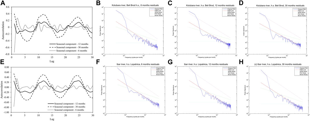
FIGURE 3. Upper row: (A) autocorrelation function for residuals of the derived models for Beli Brod station; determination of the type of colored noise for (B) 6, (C) 12 and (D) 30 months residuals (Beli Brod); Lower row: (E) autocorrelation function for residuals of the derived models for Lopatnica station; determination of the type of colored noise for 6 (F), 12 (G) and 30 (H) months residuals (Lopatnica).
We assume that landslide dynamics could be modeled as the movement of the n interconnected blocks:
where xi and yi represent displacement and velocity of the ith block, respectively, K is the constant of spring connecting the blocks, τ is time delay and V is the nondimensional pulling background velocity. Zi(t) stands for the river level oscillations represented as an Ornstein-Uhlenbeck process, and terms
Parameters a, b and c are parameters of the cubic friction force, which according to Morales et al. (2017) has the following form:
Results of the numerical analysis of the model (3) indicate the existence of two dynamical regimes.
- Equilibrium state, which manifests as steady stationary movement (corresponding to the landslide creep regime);
- Small-amplitude regular periodic oscillations (corresponding to the active phase of landslide displacement).
Results of the performed research indicate that the increase of noise intensity induces destabilization of the landslide creeping and leads to landslide activation. Such qualitative impact of the intensity of colored noise is recorded for variable values of D (in the range 10−2–10−5). One should note that no significant change in dynamics of the model (1) is observed for the change of D from 10−5 to 10−4.
It should be noted that, regarding the noise level determination, in the present paper, since model is dimensionless, noise level is also dimensionless and it is defined in two ways.
• compared to the amplitude of periodic oscillations after the bifurcation curve is crossed. In the present case, for the chosen fixed parameter values ε=1, ω=1, ξ1=ξ2=0.001, a=3.2, b=7.2, c=4.8 and set initial conditions: x1=x2=1.001, y1=y2=0.002, z1=z2=0.001, θ=0.001, amplitudes of oscillations are of order 1.5 (k=4, τ=4). When the highest assumed value of noise is introduced D=10−2, differences of oscillations with and without the assumed noise is of the order 10–4. Hence, the assumed range of noise level D=10−5 to 10−2 is significantly smaller than the compared oscillations above the bifurcation curve.
• compared to the amplitude of river level periodic oscillations. In the present case, for the chosen fixed parameter values ε=1, ω=1, ξ1=ξ2=0.001, a=3.2, b=7.2, c=4.8 and set initial conditions: x1=x2=1.001, y1=y2=0.002, z1=z2=0.001, θ=0.001, amplitudes of river level oscillations are of order 10–4 below the bifurcation curve (k=1, τ=1). From this point of view, relevant noise levels are in the range 10−4–10−5, when differences in the amplitude of river level oscillations with and without noise are of the order 10−8–10−4. Therefore, from the viewpoint of the amplitude of river level oscillations, relevant noise levels are of the order 10−5–10−4. Higher values of noise lead to the extreme case when noise level is approximately the same as the “main signal”.
For the fixed values of friction parameters, it appears that for each increase of D (for one order of unit), critical values of displacement delay and slope stiffness for which bifurcation occurs reduce by 0.1. As shown in Figure 4, bifurcation line “moves” parallel to the lower values of τ and k with the increase of noise intensity. One should note that the observed changes are happening for rather large values of displacement delay and slope stiffness, of the order 0.1, so one can interpret the recorded features as very significant, since changes induced by the change of noise intensity occur at the level of observation.
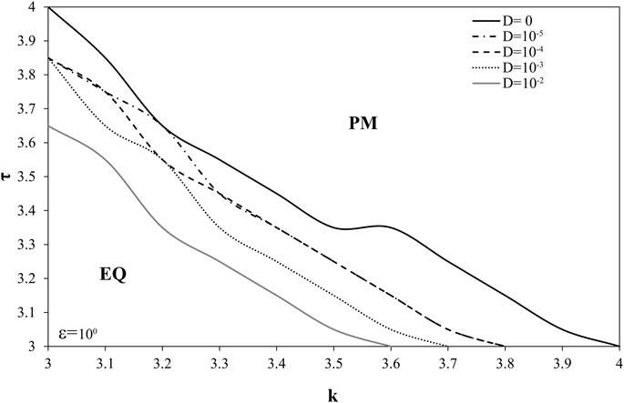
FIGURE 4. Bifurcation diagram k-τ for variable values of noise intensity D. While k, τ and D are varied, other parameters of the model (1) are being held constant: ε=1, ω=1, ξ1=ξ2=0.001, a=3.2, b=7.2, c=4.8. Initial conditions are set: x1=x2=1.001, y1=y2=0.002, z1=z2=0.001, θ=0.001.
From the geodynamical viewpoint, such findings indicate that noise intensity reduces the critical values of slope stiffness and displacement delay for which instability occurs. In other words, in the presence of colored noise landslide hazard increases.
In case when friction parameters are being varied, noise intensity has qualitatively the same effect on stability of landslide dynamics as in the previous case (Figure 5). It seems that friction parameter a is the most sensitive to the change of the noise intensity; similarly to the co-effect of delay and slope stiffness, the change of D from 10−5 to 10−2 leads to the transition of bifurcation curve down by 0.1 concerning the friction parameter a (Figure 5). It should be emphasized that the increase of noise intensity leads to destabilization of landslide dynamics.

FIGURE 5. Bifurcation diagram a-τ for variable values of noise intensity. While τ and D are varied, other parameters of the model (1) are being held constant: k=3, ε=1, ω=1, ξ1=ξ2=0.001, b=7.2, c=4.8. Initial conditions are set: x1=x2=1.001, y1=y2=0.002, z1=z2=0.001, θ=0.001.
From the geodynamical viewpoint, parameter a controls the brittle-ductile transition; in particular, the increase of parameter a in the examined range (and further) indicates a change in the slope behavior from ductile, with pronounced peak and residual shear strength, to plastic, where no clear drop of shear strength is observed.
Regarding the interaction of noise intensity with other two friction parameters, b (Figure 6A) and c (Figure 6B), results obtained indicate that these parameters are less sensitive, meaning that with the change of noise intensity only the critical value of the displacement delay changes, while the relevant values of parameter b and c remain almost the same. One could note that parameter c has qualitatively the same effect to landslide dynamics as parameter a: the increase of parameter c leads to stabilization of landslide dynamics, while noise intensity acts as a destabilizing factor. On the other hand, the increase of parameter b leads to destabilization of the landslide dynamics, with the same effect of D.
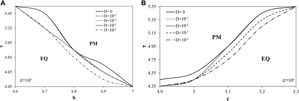
FIGURE 6. Bifurcation diagrams displacement delay-friction parameters: (A) b-τ and (B) c-τ, for variable values of noise intensity. While τ and D are varied, other parameters of the model (1) are being held constant: k=3, ε=1, ω=1, ξ1=ξ2=0.001, a=3.2, b=7.2, c=4.8. Initial conditions are set: x1=x2=1.001, y1=y2=0.002, z1=z2=0.001, θ=0.001.
Considering the observed interaction of friction parameters and noise intensity with displacement delay, one could conclude that noise intensity, although small compared to the relevant scales of other control parameters, alters the governing friction low and, for certain values of friction parameters, makes slope more susceptible to the onset of unstable landslide dynamics.
Such effect of the change of noise intensity is also observed for the case when displacement delay is held constant. It appears that for high values of D bifurcation occurs for lower values of slope stiffness and for higher values of friction parameters a (Figure 7A) and c (Figure 7B). Compared to the case of fixed friction parameters (Figure 4), the amount of change of k is almost the same for parameters b and c, while it is 2 times smaller for the case when parameter a is being varied.
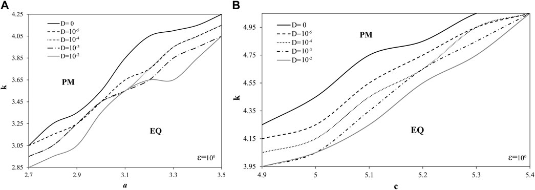
FIGURE 7. Bifurcation diagrams slope stifness-friction parameters: (A) a-k and (B) c-k, for variable values of noise intensity. While k and D are varied, other parameters of the model (1) are being held constant: τ=3, ε=1, ω=1, ξ1=ξ2=0.001, a=3.2, b=7.2, c=4.8. Initial conditions are set: x1=x2=1.001, y1=y2=0.002, z1=z2=0.001, θ=0.001.
As for the interaction of parameter b and noise intensity when displacement delay has a constant value (Figure 8), it seems that, in such case, parameter b is more sensitive to the change in D. Change of D for 4 orders of units leads to the onset of bifurcation for values of parameter b which are smaller for 0.2 units, compared to 0.05 units, in case when slope stiffness has a constant value.
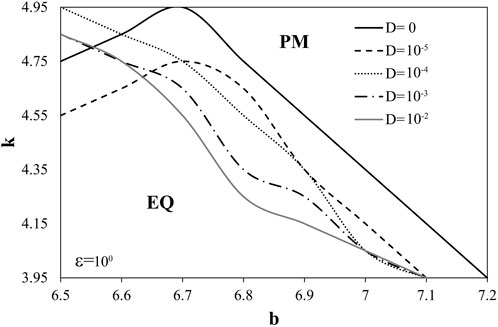
FIGURE 8. Bifurcation diagram b-k for variable values of noise intensity. While k and D are varied, other parameters of the model (1) are being held constant: τ=3, ε=1, ω=1, ξ1=ξ2=0.001, a=3.2, c=4.8. Initial conditions are set: x1=x2=1.001, y1=y2=0.002, z1=z2=0.001, θ=0.001.
Compared to the influence of noise intensity, the effect of correlation time is much less emphasized, e.g., displacement delay, spring stiffness and friction parameters are rather robust to the effect of correlation time. Nevertheless, this effect is clearly captured and confirms the significance of influence of the noise color on the landslide dynamics.
From Figure 9 one could identify the effect of correlation time ε on the dynamics of model (1). In particular, increase of correlation time ε from 0.1 to 10 leads to destabilization of landslide dynamics, but only for certain values of delay displacement (3.2 ≤ τ ≤ 3.4) and slope stiffness (3.3 ≤ τ ≤ 3.5). This further means the effect of correlation time is not generic, but could occur only for certain values of delay and stiffness.
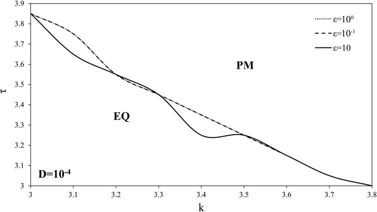
FIGURE 9. Bifurcation diagram k-τ for variable values of correlation time ε. While k, τ and ε are varied, other parameters of the model (1) are being held constant: D=10−4, ω=1, ξ1=ξ2=0.001, a=3.2, b=7.2, c=4.8. Initial conditions are set: x1=x2=1.001, y1=y2=0.002, z1=z2=0.001, θ=0.001.
Regarding the interaction of correlation time and friction parameters, results obtained indicate that friction parameter b is robust to the change of correlation time in the range from 0.1 to 10. Some weak sensitivity to change of correlation time is captured for friction parameter a, where the increase of correlation time actually leads to stabilization of landslide dynamics (Figure 10A). Such effect of correlation time is opposite to the effect of noise intensity. From the geodynamical viewpoint, it means that degree of noise correlation could be crucial for the stability of landslide dynamics. As for the friction parameter c, it seems that nature of the effect of correlation time change also changes with the increase of parameter c (Figure 10). For low values of parameter c, increase of correlation time leads to stabilization of landslide dynamics, i.e., such effect is opposite to the effect of the noise intensity. For higher values of c, increase of correlation time leads to destabilization of landslide dynamics, which is qualitatively the same effect as the noise intensity.
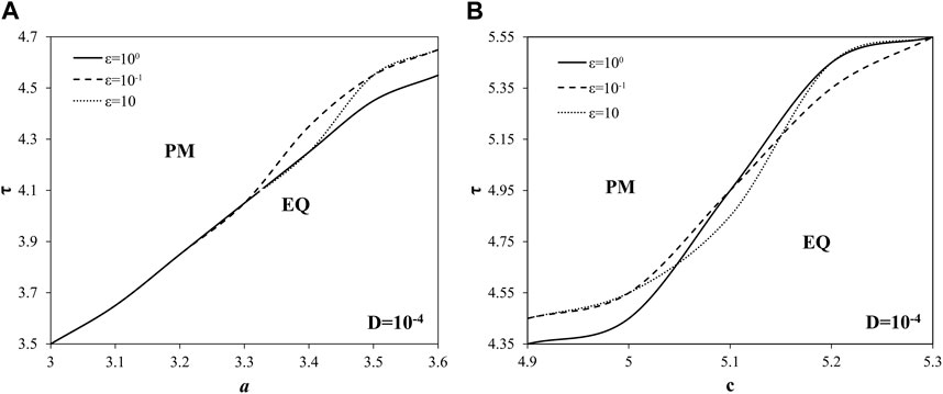
FIGURE 10. Bifurcation diagrams time delay-friction parameters: (A) a-τ, (B) b-τ and (C) c-τ, for variable values of correlation time ε. While τ and ε are varied, other parameters of the model (1) are being held constant: D=10−4, k=3, ω=1, ξ1=ξ2=0.001, a=3.2, b=7.2, c=4.8. Initial conditions are set: x1=x2=1.001, y1=y2=0.002, z1=z2=0.001, θ=0.001.
Stabilizing effect of the correlation time is more clearly seen for the constant value of displacement delay (Figure 11). As for the interaction of friction parameters b and c and the change of correlation time when displacement delay is fixed, the same destabilizing effect is captured both for parameters b and c (Figure 12).
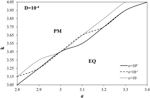
FIGURE 11. Bifurcation diagrams spring stifness-friction parameter k-a for variable values of correlation time ε. While k, a and ε are varied, other parameters of the model (1) are being held constant: D=10−4, k=3, ω=1, ξ1=ξ2=0.001, a=3.2, b=7.2, c=4.8. Initial conditions are set: x1=x2=1.001, y1=y2=0.002, z1=z2=0.001, θ=0.001.
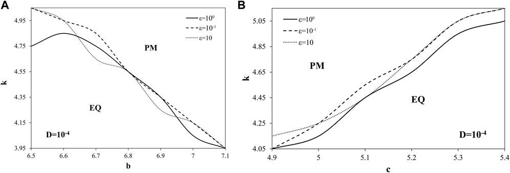
FIGURE 12. Bifurcation diagrams slope stiffness-friction parameters: (A) b-k and (B) c-k, for variable values of correlation time ε. While b, c, k and ε are varied, other parameters of the model (1) are being held constant: τ=3, D=10−4, ω=1, ξ1=ξ2=0.001, b=7.2, c=4.8. Initial conditions are set: x1=x2=1.001, y1=y2=0.002, z1=z2=0.001, θ=0.001.
In present paper, we examine the impact of colored noise in river level oscillations on the landslide dynamics. Firstly, we prove, by analyzing the measurement of the river oscillation recordings, that noise in river level oscillations could be treated as the colored noise. This is done for the recordings made at two different hydrological stations in Serbia: Beli Brod station (the Kolubara river) and Lopatnica Lakat station (the Ibar river). We examined available water level recordings for the Kolubara river and the Ibar river for the periods 1959–2007 and 1948–2007, respectively. By applying LOESS method and spectral analysis, we derived deterministic models for the recorded time series, which are proved to be statistically significant. At the end of the first phase of the research, it is shown that residuals of derived models could be characterized as an example of colored noise. In that way, we justified the introduction of both the deterministic water level oscillation and low-magnitude color noise into the model of landslide dynamics.
In the second phase of the research, we investigate the landslide dynamics by analyzing the model of two coupled blocks, with displacement delay and with the assumed additive colored noise. The results obtained indicate the existence of two different dynamical regimes, all of which could have its correspondence with the real observed regimes of landslide dynamics: (1) steady stationary state (creep regime); and (2) active landslide dynamics. The results indicate significant effect of noise intensity and correlation on the onset of unstable landslide dynamics. In particular, increase of noise intensity leads to destabilization of landslide dynamics, in the following way.
- noise intensity reduces the critical values of slope stiffness and displacement delay for which instability occurs,
- it seems that friction parameter a is the most sensitive to the change of the noise intensity; since parameter a controls the ductile-plastic transition, it could be said that the change in the colored noise actually alters deformable properties of the slope,
- effect of correlation time is much less emphasized, in a way that displacement delay, spring stiffness and friction parameters are rather robust to the effect of correlation time,
- some weak sensitivity to change of correlation time is captured for friction parameter a, where the increase of correlation time actually leads to stabilization of landslide dynamics. Such effect of correlation time is opposite to the effect of noise intensity.
If one compares the effect of colored noise, analyzed in this paper, and random noise, analyzed in our previous paper (Kostić et al., 2023), the difference lies in the following. For random background noise, we confirmed its stabilizing effect on the landslide dynamics. In particular, in our previous paper (Kostić et al., 2023) noise has the same effect for highly weathered rock masses, with rather low values of spring stiffness and high values of time delay, and for slightly weathered rock masses, with high values of spring stiffness and low values of time delay. On the other hand, in present paper we show that noise intensity, although small compared to the relevant scales of other control parameters, alters the governing friction low and, for certain values of friction parameters, makes slope more susceptible to the onset of unstable landslide dynamics. Also, we show that correlation time could also have significant effect, even opposite to the effect of noise intensity, which further confirms the significance of the color of noise on landslide dynamics.
It could be interesting to briefly discuss the possible natural roots of the increased noise intensity in the river level fluctuations. Root of noise in river level oscillations in general could be considered as the product by a combination of geographic, hydroclimatic and anthropogenic variables, which was also previously suggested by Tu et al. (2023) as a possible cause of spatial variation in noise colour of daily and annual river flow. Increase of noise in river water levels could be attributed to both seasonal and multi-annual climate variabilities. While seasonal variability consistently affects annual water level patterns, it is the prolonged climate variability, particularly arising from atmosphere-ocean oscillation, that profoundly influences flood-related dynamics (Kundzewicz et al., 2019). Such variability is postulated to be a fundamental factor of spatial and temporal shifts in hydrometeorological variables across Europe (Nobre et al., 2017). Also, torrential floods could be the cause of the increase of noise level. In particular, low-frequency climate variations have been linked to genesis of flash floods (Archer et al., 2019), where swift of flood events is recognized to be a consequence of morphological, pedological, geological, and climatic attributes of specific torrential basins. In the present paper, goal of the research was to indicate that when slope is in critical state (near the bifurcation), even small increase in noise amplitude within the river level oscillations could lead to occurrence of instability.
It should be noted that the performed analysis is conducted for the initial conditions near the equilibrium state; hence, only the local dynamics of the landslide model is examined. Possible occurrence of global bifurcations when initial conditions are away from the equilibrium state (possible occurrence of global bifurcations) was not investigated in the present paper. Further work on this topic could include the analysis of other local bifurcation curves, or the possible existence of global bifurcation, which could eventually lead to definition of conditions for the occurrence of stick-slip dynamics, which is qualitatively the most resemblant to the real unstable dynamics.
The raw data supporting the conclusion of this article will be made available by the authors, without undue reservation.
SK: Formal Analysis, Investigation, Writing–original draft. MS: Formal Analysis, Investigation, Resources, Writing–original draft.
The author(s) declare that no financial support was received for the research, authorship, and/or publication of this article.
The authors declare that the research was conducted in the absence of any commercial or financial relationships that could be construed as a potential conflict of interest.
All claims expressed in this article are solely those of the authors and do not necessarily represent those of their affiliated organizations, or those of the publisher, the editors and the reviewers. Any product that may be evaluated in this article, or claim that may be made by its manufacturer, is not guaranteed or endorsed by the publisher.
Abam, T. K. S. (1993). Factors affecting distribution of instability of river banks in the Niger delta. Eng. Geol. 35, 123–133. doi:10.1016/0013-7952(93)90074-m
Archer, D., O'donnell, G., Lamb, R., Warren, S., and Fowler, H. J. (2019). Historical flash floods in England: new regional chronologies and database. J- Flood Risk Manag. 12, e12526. doi:10.1111/jfr3.12526
Chen, C. H., Hsieh, T. Y., and Yang, J. C. (2017). Investigating effect of water level variation and surface tension crack on riverbank stability. J. Hydro-Environ. Res. 15, 41–53. doi:10.1016/j.jher.2017.02.002
Dapporto, S., Rinaldi, M., and Casagli, N. (2001). Failure mechanisms and pore water pressure conditions: analysis of a riverbank along the Arno River (Central Italy). Eng. Geol. 61, 221–242. doi:10.1016/s0013-7952(01)00026-6
Duong, T. T., and Do, M. D. (2019). Riverbank stability assessment under river water level changes and hydraulic erosion. Water 11, 2598. doi:10.3390/w11122598
Duong, T. T., Komine, H., Do, M. D., and Murakami, S. (2014). Riverbank stability assessment under flooding conditions in the Red River of Hanoi, vietnam. Comput. Geotechnics 61, 178–189. doi:10.1016/j.compgeo.2014.05.016
Ghil, M., Yiou, P., Hallegatte, S., Malamud, B. D., Naveau, P., Soloviev, A., et al. (2011). Extreme events: dynamics, statistics and prediction. Nonlinear Process Geophys 18, 295–350. doi:10.5194/npg-18-295-2011
Hurst, H. E. (1951). Long-term storage capacity of reservoirs. Trans. Am. Soc. Civ. Eng. 116, 770–799. doi:10.1061/taceat.0006518
Koscielny-Bunde, E., Kantelhardt, J. W., Braun, P., Bunde, A., and Havlin, S. (2006). Long-term persistence and multifractality of river runoff records: detrended fluctuation studies. J. Hydrol. 322, 120–137. doi:10.1016/j.jhydrol.2005.03.004
Kostić, S., Stojković, M., Guranov, I., and Vasović, N. (2019). Revealing the background of groundwater level dynamics: contributing factors, complex modeling and engineering applications. Chaos, Solit. Fract. 127, 408–421. doi:10.1016/j.chaos.2019.07.007
Kostić, S., Vasović, N., Todorović, K., and Franović, I. (2020). Effect of colored noise on the generation of seismic fault movement: analogy with spring-block model dynamics. Chaos Solit. Fract. 135, 109726. doi:10.1016/j.chaos.2020.109726
Kostić, S., Vasović, N., Todorović, K., and Prekrat, D. (2023). Instability induced by random background noise in a delay model of landslide dynamics. Appl. Sci. 13, 6112. doi:10.3390/app13106112
Kundzewicz, Z. W., Szwed, M., and Pińskwar, I. (2019). Climate variability and floods—a global review. Water 11 (7), 1399. doi:10.3390/w11071399
Liang, C., Jaksa, M., Ostendorf, B., and Kuo, Y. (2015). Influence of river level fluctuations and climate on riverbank stability. Comput. Geotech. 63, 83–98. doi:10.1016/j.compgeo.2014.08.012
Mentes, G. (2019). Relationship between river bank stability and hydrological processes using in situ measurement data. Cent. Eur. Geol. 62, 83–99. doi:10.1556/24.62.2019.01
Morales, J. E. M., James, G., and Tonnelier, A. (2017). Traveling waves in a spring-block chain sliding down a slope. Phys. Rev.E 96, 012227. doi:10.1103/physreve.96.012227
Nobre, G. G., Jongman, B., Aerts, J. C. J. H., and Ward, P. J. (2017). The role of climate variability in extreme floods in Europe. Environ. Res. Lett. 12 (8), 084012. doi:10.1088/1748-9326/aa7c22
Stojković, M., Kostić, S., Plavšić, J., and Prohaska, S. (2017). A joint stochastic-deterministic approach for long-term and short-term modelling of monthly flow rates. J. Hydrol. 544, 555–566. doi:10.1016/j.jhydrol.2016.11.025
Tu, T., Comte, L., and Ruhi, A. (2023). The color of environmental noise in river networks. Nat. Commun. 14, 1728. doi:10.1038/s41467-023-37062-2
Újvári, G., Mentes, G., Bányai, L., Kraft, J., Gyimóthy, A., and Kovács, J. (2009). Evolution of a bank failure along the river Danube at dunaszekcső, Hungary. Geomorph 109, 197–209. doi:10.1016/j.geomorph.2009.03.002
Vračar, M. S., and Mijić, M. (2011). Ambient noise in large rivers (L). J. Acoust. Soc. Am. 130, 1787–1791. doi:10.1121/1.3628666
Keywords: landslide, spring-block model, colored noise, noise intensity, correlation time, delayed interaction, bifurcation
Citation: Kostić S and Stojković M (2023) Colored noise in river level oscillations as triggering factor for unstable dynamics in a landslide model with displacement delay. Front. Earth Sci. 11:1267225. doi: 10.3389/feart.2023.1267225
Received: 26 July 2023; Accepted: 24 October 2023;
Published: 08 November 2023.
Edited by:
Yi Xue, Xi’an University of Technology, ChinaReviewed by:
Annette Witt, Max Planck Society, GermanyCopyright © 2023 Kostić and Stojković. This is an open-access article distributed under the terms of the Creative Commons Attribution License (CC BY). The use, distribution or reproduction in other forums is permitted, provided the original author(s) and the copyright owner(s) are credited and that the original publication in this journal is cited, in accordance with accepted academic practice. No use, distribution or reproduction is permitted which does not comply with these terms.
*Correspondence: Srđan Kostić, c3JkamFuLmtvc3RpY0BqY2VybmkucnM=
Disclaimer: All claims expressed in this article are solely those of the authors and do not necessarily represent those of their affiliated organizations, or those of the publisher, the editors and the reviewers. Any product that may be evaluated in this article or claim that may be made by its manufacturer is not guaranteed or endorsed by the publisher.
Research integrity at Frontiers
Learn more about the work of our research integrity team to safeguard the quality of each article we publish.