Computational aspects of the equivalent-layer technique: review

Equivalent-layer technique is a powerful tool for processing potential-field data in the space domain. However, the greatest hindrance for using the equivalent-layer technique is its high computational cost for processing massive data sets. The large amount of computer memory usage to store the full sensitivity matrix combined with the computational time required for matrix-vector multiplications and to solve the resulting linear system, are the main drawbacks that made unfeasible the use of the equivalent-layer technique for a long time. More recently, the advances in computational power propelled the development of methods to overcome the heavy computational cost associated with the equivalent-layer technique. We present a comprehensive review of the computation aspects concerning the equivalent-layer technique addressing how previous works have been dealt with the computational cost of this technique. Historically, the high computational cost of the equivalent-layer technique has been overcome by using a variety of strategies such as: moving data-window scheme, column- and row-action updates of the sensitivity matrix, reparametrization, sparsity induction of the sensitivity matrix, iterative methods using the full sensitivity matrix, iterative deconvolution by using the concept of block-Toeplitz Toeplitz-block (BTTB) matrices and direct deconvolution. We compute the number of floating-point operations of some of these strategies adopted in the equivalent-layer technique to show their effectiveness in reducing the computational demand. Numerically, we also address the stability of some of these strategies used in the equivalent-layer technique by comparing with the stability via the classic equivalent-layer technique with the zeroth-order Tikhonov regularization. We show that even for the most computationally efficient methods, which can save up to 10⁹ flops, the stability of the linear system is maintained. The two most efficient strategies, iterative and direct deconvolutions, can process large datasets quickly and yield good results. However, direct deconvolution has some drawbacks. Real data from Carajás Mineral Province, Brazil, is also used to validate the results showing a potential field transformation.

1 Introduction

The equivalent-layer technique has been used by exploration geophysicists for processing potential-field data since the late 1960s (Dampney, 1969). This technique is based on a widely accepted principle, which states that a discrete set of observed potential-field data due to 3D sources can be approximated by that due to a discrete discrete set of virtual sources (such as point masses, dipoles, prisms, doublets). From a theoretical point of view, the equivalent-layer technique is grounded on potential theory (Kellogg, 1967) and consists in considering that the potential field data can be approximated by a linear combination of harmonic functions describing the potential field due to the virtual sources. These sources, commonly called equivalent sources, are arranged on a layer with finite horizontal dimensions and located below the observations. In the classical approach, a linear inverse problem is solved to estimate the physical property of each equivalent source subject to fit the observations. Then, the estimated physical-property distribution on the equivalent layer is used to accomplish the desired potential-field transformation (e.g., interpolation, upward/downward continuation, reduction to the pole). The later step is done by multiplying the estimated physical-property distribution by the matrix of Green’s functions associated with the desired potential-field transformation.

Because the linear inverse problem to be solved in the equivalent-layer technique is set up with a full sensitivity matrix, its computational cost strongly depends on the number of potential-field observations and can be very inefficient for dealing with massive data sets. To overcome this problem, computationally efficient methods based on equivalent-layer technique have arose in the late 1980s. This comprehensive review discusses specific strategies aimed at reducing the computational cost of the equivalent-layer technique. These strategies are addressed in the following articles: Leão and Silva (1989); Cordell (1992); Xia et al. (1993); Mendonça and Silva (1994); Guspí and Novara (2009); Li and Oldenburg (2010); Oliveira Jr. et al. (2013); Siqueira et al. (2017); Jirigalatu and Ebbing (2019); Takahashi et al. (2020, 2022) Mendonça (2020); and Soler and Uieda (2021);

To our knowledge, the first method towards improving the efficiency was proposed by Leão and Silva (1989), who used an overlapping moving-window scheme spanning the data set. The strategy adopted in Leão and Silva (1989) involves solving several smaller, regularized linear inverse problems instead of one large problem. This strategy uses a small data window and distributes equivalent sources on a small regular grid at a constant depth below the data surface, with the sources’ window extending beyond the boundaries of the data window. Because of the spatial layouts of observed data and equivalent sources in Leão and Silva (1989), the small sensitivity submatrix containing the coordinates of the data and equivalent sources within a window remains constant for all data windows. This holds true regardless of the specific locations of the data and equivalent sources within each window. For each position of the data window, this scheme consists in computing the processed field at the center of the data window only, and the next estimates of the processed field are obtained by shifting the data window across the entire dataset. More recently, Soler and Uieda (2021) extended the method introduced by Leão and Silva (1989) to accommodate irregularly spaced data collected on a non-flat surface. Unlike Leão and Silva (1989), in the generalization proposed by Soler and Uieda (2021), the sensitivity submatrix that includes the coordinates of the data and equivalent sources needs to be computed for each window. Soler and Uieda (2021) developed a computational approach to further enhance the efficiency of the equivalent-layer technique by combining two strategies. The first one—the block-averaging source locations—reduces the number of model parameters and the second strategy—the gradient-boosted algorithm—reduces the size of the linear system to be solved by iteratively fitting the equivalent source model along overlapping windows. It is worth noting that the equivalent-layer strategy of using a moving-window scheme either in Leão and Silva (1989) or in Soler and Uieda (2021) is similar to discrete convolution.

As another strategy to reduce the computational workload of the equivalent-layer technique, some authors have employed column- and row-action updates, which are commonly applied to image reconstruction methods (e.g., Elfving et al., 2017). These methods involve iterative calculations of a single column and a single row of the sensitivity matrix, respectively. Following the strategy column-action update, Cordell (1992) proposed a computational method in which a single equivalent source positioned below a measurement station is iteratively used to compute both the predicted data and residual data for all stations. In Cordell’s method, a single column of the sensitivity matrix is calculated per iteration, meaning that a single equivalent source contributes to data fitting in each iteration. Guspí and Novara (2009) further extended Cordell’s method by applying it to scattered magnetic observations. Following the strategy of column-action update, Mendonça and Silva (1994) developed an iterative procedure where one data point is incorporated at a time, and a single row of the sensitivity matrix is calculated per iteration. This strategy adopted by Mendonça and Silva (1994) is known as equivalent data concept. This concept is based on the principle that certain data points within a dataset are redundant and, as a result, do not contribute to the final solution On the other hand, there is a subset of observations known as equivalent data, which effectively contributes to the final solution and fits the remaining redundant data. In their work, Mendonça and Silva (1994) adopted an iterative approach to select a substantially smaller subset of equivalent data from the original dataset.

The next strategy involves reparametrizing the equivalent layer with the objective of solving a smaller linear inverse problem by reducing the dimension of the model space. Oliveira Jr. et al. (2013) reduced the model parameters by approximating the equivalent-source layer by a piecewise-polynomial function defined on a set of user-defined small equivalent-source windows. The estimated parameters are the polynomial coefficients for each window and they are much smaller than the original number of equivalent sources. By using the subspace method, Mendonça (2020) reparametrizes the equivalent layer, which involves reducing the dimension of the linear system from the original parameter-model space to a lower-dimensional subspace. The subspace bases span the parameter-model space and they are constructed by applying the singular value decomposition to the matrix containing the gridded data.

Following the strategy of sparsity induction, Li and Oldenburg (2010) transformed the full sensitivity matrix into a sparse one using orthonormal compactly supported wavelets. Barnes and Lumley (2011) proposed an alternative approach to introduce sparsity based on the use of quadtree discretization to group equivalent sources far from the computation points. Those authors explore the induced sparsity by using specific iterative methods to solve the linear system.

The strategy named iterative methods estimates iteratively the parameter vector that represents a distribution over an equivalent layer. Xia and Sprowl (1991) and Xia et al. (1993) have developed efficient iterative algorithms for updating the distribution of physical properties within the equivalent layer in the wavenumber and space domains, respectively. Specifically, in Xia and Sprowl’s (1991) method the physical-property distribution is updated by using the ratio between the squared depth to the equivalent source and the gravitational constant multiplied by the residual between the observed and predicted observation at the measurement station. Siqueira et al. (2017) developed an iterative solution where the sensitivity matrix is transformed into a diagonal matrix with constant terms through the use of the excess mass criterion and of the positive correlation between the observed gravity data and the masses on the equivalent layer. The fundamentals of the Siqueira et al.’s method is based on the Gauss’ theorem (e.g., Kellogg, 1967, p. 43) and the total excess of mass (e.g., Blakely, 1996, p. 60). All these iterative methods use the full and dense sensitivity matrix to calculate the predicted data and residual data in the whole survey data per iteration. Hence, the iterative methods proposed by Xia and Sprowl (1991), Xia et al. (1993) and Siqueira et al. (2017) neither compress nor reparametrize the sensitivity matrix. Jirigalatu and Ebbing (2019) also proposed an iterative equivalent layer that uses the full and dense sensitivity matrix. However, in their approach, Jirigalatu and Ebbing (2019) efficiently compute the predicted data and residual data for the entire survey per iteration in the wavenumber domain.

Following the strategy of the iterative deconvolution, Takahashi et al. (2020, 2022) developed fast and effective equivalent-layer techniques for processing, respectively, gravity and magnetic data by modifying the forward modeling to estimate the physical-property distribution over the equivalent layer through a 2D discrete fast convolution. These methods took advantage of the Block-Toeplitz Toeplitz-block (BTTB) structure of the sensitivity matrices, allowing them to be calculated by using only their first column. In practice, the forward modeling uses a single equivalent source, which significantly reduces the required RAM memory.

The method introduced by Takahashi et al. (2020, 2022) can be reformulated to eliminate the need for conjugate gradient iterations. This reformulation involves employing a direct deconvolution approach (e.g., Aster et al., 2019, p. 220) with Wiener filter (e.g., Gonzalez and Woods, 2002, p. 263).

Here, we present a comprehensive review of diverse strategies to solve the linear system of the equivalent layer alongside an analysis of the computational cost and stability of these strategies. To do this analysis, we are using the floating-point operations count to evaluate the performance of a selected set of methods (e.g., Leão and Silva (1989); Cordell (1992); Oliveira Jr. et al. (2013); Siqueira et al. (2017); Mendonça (2020); Takahashi et al. (2020); Soler and Uieda (2021); and direct deconvolution). To test the stability, we are using the linear system sensitivity to noise as a comparison parameter for the fastest of these methods alongside the classical normal equations. A potential-field transformation will also be used to evaluate the quality of the equivalent sources estimation results using both synthetic and real data from Carajás Mineral Province, Brazil.

In the following sections, we will address the theoretical bases of the equivalent-layer technique, including aspects such as the sensitivity matrix, layer depth and spatial distribution and the total number of equivalent sources. Then, we will explore the general formulation and solution of the linear inverse problem for the equivalent-layer technique, including discussions on linear system solvers. Additionally, we will quantify the required arithmetic operations for a given equivalent-layer method, assessing the number of floating-point operations involved. Next, we will evaluate the stability of the estimated solutions obtained from applying specific equivalent-layer methods. Finally, we will delve into the computational strategies adopted in the equivalent-layer technique for reducing computational costs. These strategies encompass various approaches, such as the moving data-window scheme, column-and row-action updates of the sensitivity matrix, reparametrization, sparsity induction of the sensitivity matrix, iterative methods using the full sensitivity matrix, iterative deconvolution using the concept of block-Toeplitz Toeplitz-block (BTTB) matrices, and direct deconvolution.

2 Fundamentals

Let d be a D × 1 vector, whose ith element d_i is the observed potential field at the position (x_i, y_i, z_i), i ∈ {1: D}, of a topocentric Cartesian system with x, y and z-axes pointing to north, east and down, respectively. Consider that d_i can be satisfactorily approximated by a harmonic function

$f_i={\displaystyle \sum _{j=1}^P}{g}_{ij}{p}_j,i\in \left\{1:D\right\},(1)$

where, p_j represents the scalar physical property of a virtual source (i.e., monopole, dipole, prism) located at (x_j, y_j, z_j), j ∈ {1: P} and

$g_{ij}\equiv g\left(x_i-x_j,y_i-y_j,z_i-z_j\right),z_i<\min \left\{z_j\right\},\forall i\in \left\{1:D\right\},(2)$

is a harmonic function, where min{z_j} denotes the minimum z_j, or the vertical coordinate of the shallowest virtual source. These virtual sources are called equivalent sources and they form an equivalent layer. In matrix notation, the potential field produced by all equivalent sources at all points (x_i, y_i, z_i), i ∈ {1: D}, is given by:

$\mathbf{f}=\mathbf{G}\mathbf{p},(3)$

where p is a P × 1 vector with jth element p_j representing the scalar physical property of the jth equivalent source and G is a D × P matrix with element g_ij given by Eq. 2.

The equivalent-layer technique consists in solving a linear inverse problem to determine a parameter vector p leading to a predicted data vector f (Eq. 3) sufficiently close to the observed data vector d, whose ith element d_i is the observed potential field at (x_i, y_i, z_i). The notion of closeness is intrinsically related to the concept of vector norm (e.g., Golub and Van Loan, 2013, p. 68) or measure of length (e.g., Menke, 2018, p. 41). Because of that, almost all methods for determining p actually estimate a parameter vector $\tilde{\mathbf{p}}$ minimizing a length measure of the difference between f and d (see Subsection 3.1). Given an estimate $\tilde{\mathbf{p}}$, it is then possible to compute a potential field transformation

$\mathbf{t}=\mathbf{A}\tilde{\mathbf{p}},(4)$

where t is a T × 1 vector with kth element t_k representing the transformed potential field at the position (x_k, y_y, z_k), k ∈ {1: T}, and

$a_{kj}\equiv a\left(x_k-x_j,y_k-y_j,z_k-z_j\right),z_k<\min \left\{z_j\right\},\forall k\in \left\{1:T\right\},(5)$

is a harmonic function representing the kj-th element of the T × P matrix A.

2.1 Spatial distribution and total number of equivalent sources

There is no well-established criteria to define the optimum number P or the spatial distribution of the equivalent sources. We know that setting an equivalent layer with more (less) sources than potential-field data usually leads to an underdetermined (overdetermined) inverse problem (e.g., Menke, 2018, p. 52–53). Concerning the spatial distribution of the equivalent sources, the only condition is that they must rely on a surface that is located below and does not cross that containing the potential field data Soler and Uieda (2021) present a practical discussion about this topic.

From a theoretical point of view, the equivalent layer reproducing a given potential field data set cannot cross the true gravity or magnetic sources. This condition is a consequence of recognizing that the equivalent layer is essentially an indirect solution of a boundary value problem of potential theory (e.g., Roy, 1962; Zidarov, 1965; Dampney, 1969; Li et al., 2014; Reis et al., 2020). In practical applications, however, there is no guarantee that this condition is satisfied. Actually, its is widely known from practical experience (e.g., Gonzalez et al., 2022) that the equivalent-layer technique works even for the case in which the layer cross the true sources.

Regarding the depth of the equivalent layer, Dampney (1969) proposed a criterion based on horizontal data sampling, suggesting that the equivalent-layer depth should be between two and six times the horizontal grid spacing, considering evenly spaced data. However, when dealing with a survey pattern that has unevenly spaced data, Reis et al. (2020) adopted an alternative empirical criterion. According to their proposal, the depth of the equivalent layer should range from two to three times the spacing between adjacent flight lines. The criteria of Dampney (1969) and Reis et al. (2020) are valid for planar equivalent layers. Cordell (1992) have proposed and an alternative criterion for scattered data that leads to an undulating equivalent layer. This criterion have been slightly modified by Guspí et al. (2004), Guspí and Novara (2009) and Soler and Uieda (2021), for example, and consists in setting one equivalent source below each datum at a depth proportional to the horizontal distance to the nearest neighboring data points. Soler and Uieda (2021) have compared different strategies for defining the equivalent sources depth for the specific problem of interpolating gravity data, but they have not found significant differences between them. Regarding the horizontal layout, Soler and Uieda (2021) proposed the block-averaged sources locations in which the survey area is divided into horizontal blocks and one single equivalent source is assigned to each block. The horizontal coordinates of the single source in a given block is defined by the average horizontal coordinates of the observation points at the block. According to Soler and Uieda (2021), this block-averaged layout may prevent aliasing of the interpolated values, specially when the observations are unevenly sampled. This strategy also reduces the number of equivalent sources without affecting the accuracy of the potential-field interpolation. Besides, it reduces the computational load for estimating the physical property on the equivalent layer.

2.2 Matrix $\mathbf{G}$

Generally, the harmonic function g_ij (Eq. 2) is defined in terms of the inverse distance between the observation point (x_i, y_i, z_i) and the jth equivalent source at (x_j, y_j, z_j),

$\frac{1}{r_{ij}}\equiv \frac{1}{\sqrt{{\left(x_i-x_j\right)}^2+{\left(y_i-y_j\right)}^2+{\left(z_i-z_j\right)}^2}},(6)$

or by its partial derivatives of first and second orders, respectively given by

${\partial }_{\alpha }\frac{1}{r_{ij}}\equiv \frac{-\left({\alpha }_i-{\alpha }_j\right)}{r_{ij}^3},\alpha \in \left\{x,y,z\right\},(7)$

and

${\partial }_{\alpha \beta }\frac{1}{r_{ij}}\equiv \left\{\begin{array}{cc}\frac{3{\left({\alpha }_i-{\alpha }_j\right)}^2}{r_{ij}^5},\hfill & \alpha =\beta ,\hfill \\ \frac{3\left({\alpha }_i-{\alpha }_j\right)\left({\beta }_i-{\beta }_j\right)}{r_{ij}^5}-\frac{1}{r_{ij}^3},\hfill & \alpha \ne \beta ,\hfill \end{array}\right.\alpha ,\beta \in \left\{x,y,z\right\}.(8)$

In this case, the equivalent layer is formed by punctual sources representing monopoles or dipoles (e.g., Dampney, 1969; Emilia, 1973; Leão and Silva, 1989; Cordell, 1992; Oliveira Jr. et al., 2013; Siqueira et al., 2017; Reis et al., 2020; Takahashi et al., 2020; Soler and Uieda, 2021; Takahashi et al., 2022). Another common approach consists in not defining g_ij by using Eqs. 6–8, but other harmonic functions obtained by integrating them over the volume of regular prisms (e.g., Li and Oldenburg, 2010; Barnes and Lumley, 2011; Li et al., 2014; Jirigalatu and Ebbing, 2019). There are also some less common approaches defining the harmonic function g_ij (Eq. 2) as the potential field due to plane faces with constant physical property (Hansen and Miyazaki, 1984), doublets (Silva, 1986) or by computing the double integration of the inverse distance function with respect to z (Guspí and Novara, 2009).

A common assumption for most of the equivalent-layer methods is that the harmonic function g_ij (Eq. 2) is independent on the actual physical relationship between the observed potential field and their true sources (e.g., Cordell, 1992; Guspí and Novara, 2009; Li et al., 2014). Hence, g_ij can be defined according to the problem. The only condition imposed to this function is that it decays to zero as the observation point (x_i, y_i, z_i) goes away from the position (x_j, y_j, z_j) of the jth equivalent source. However, several methods use a function g_ij that preserves the physical relationship between the observed potential field and their true sources. For the case in which the observed potential field is gravity data, g_ij is commonly defined as a component of the gravitational field produced at (x_i, y_i, z_i) by a point mass or prism located at (x_j, y_j, z_j), with unit density. On the other hand, g_ij is commonly defined as a component of the magnetic induction field produced at (x_i, y_i, z_i) by a dipole or prism located at (x_j, y_j, z_j), with unit magnetization intensity, when the observed potential field is magnetic data.

The main challenge in the equivalent-layer technique is the computational complexity associated with handling large datasets. This complexity arises because the sensitivity matrix G (Eq. 3) is dense regardless of the harmonic function g_ij (Eq. 2) employed. In the case of scattered potential-field data, the structure of G is not well-defined, regardless of the spatial distribution of the equivalent sources. However, in a specific scenario where 1) each potential-field datum is directly associated with a single equivalent source located directly below it, and 2) both the data and sources are based on planar and regularly spaced grids, Takahashi et al. (2020, 2022) demonstrate that G exhibits a block-Toeplitz Toeplitz-block (BTTB) structure. In such cases, the product of G and an arbitrary vector can be efficiently computed using a 2D fast Fourier transform as a discrete convolution.

3 Linear inverse problem of equivalent-layer technique

3.1 General formulation

A general formulation for almost all equivalent-layer methods can be achieved by first considering that the P × 1 parameter vector p (Eq. 3) can be reparameterized into a Q × 1 vector q according to:

$\mathbf{p}=\mathbf{H}\mathbf{q},(9)$

where H is a P × Q matrix. The predicted data vector f (Eq. 3) can then be rewritten as follows:

$\mathbf{f}=\mathbf{G}\mathbf{H}\mathbf{q}.(10)$

Note that the original parameter vector p is defined in a P-dimensional space whereas the reparameterized parameter vector q (Eq. 9) lies in a Q-dimensional space. For convenience, we use the terms P-space and Q-space to designate them.

In this case, the problem of estimating a parameter vector $\tilde{\mathbf{p}}$ minimizing a length measure of the difference between f (Eq. 3) and d is replaced by that of estimating an auxiliary vector $\tilde{\mathbf{q}}$ minimizing the goal function

$\mathrm{\Gamma }\left(\mathbf{q}\right)=\mathrm{\Phi }\left(\mathbf{q}\right)+\mu \mathrm{\Theta }\left(\mathbf{q}\right),(11)$

which is a combination of particular measures of length given by

$\mathrm{\Phi }\left(\mathbf{q}\right)={\left(\mathbf{d}-\mathbf{f}\right)}^{\top }{\mathbf{W}}_d\left(\mathbf{d}-\mathbf{f}\right),(12)$

and

$\mathrm{\Theta }\left(\mathbf{q}\right)={\left(\mathbf{q}-\bar{\mathbf{q}}\right)}^{\top }{\mathbf{W}}_q\left(\mathbf{q}-\bar{\mathbf{q}}\right),(13)$

where the regularization parameter μ is a positive scalar controlling the trade-off between the data-misfit function Φ(q) and the regularization function Θ(q); W_d is a D × D symmetric matrix defining the relative importance of each observed datum d_i; W_q is a Q × Q symmetric matrix imposing prior information on q; and $\bar{\mathbf{q}}$ is a Q × 1 vector of reference values for q that satisfies

$\bar{\mathbf{p}}=\mathbf{H}\bar{\mathbf{q}},(14)$

where $\bar{\mathbf{p}}$ is a P × 1 vector containing reference values for the original parameter vector p.

After obtaining an estimate $\tilde{\mathbf{q}}$ for the reparameterized parameter vector q (Eq. 9), the estimate $\tilde{\mathbf{p}}$ for the original parameter vector (Eq. 3) is computed by

$\tilde{\mathbf{p}}=\mathbf{H}\tilde{\mathbf{q}}.(15)$

The reparameterized vector $\tilde{\mathbf{q}}$ is obtained by first computing the gradient of Γ(q),

$\mathbf{\nabla }\mathrm{\Gamma }\left(\mathbf{q}\right)=-2{\mathbf{H}}^{\top }{\mathbf{G}}^{\top }{\mathbf{W}}_d\left(\mathbf{d}-\mathbf{f}\right)+2\mu {\mathbf{W}}_q\left(\mathbf{q}-\bar{\mathbf{q}}\right).(16)$

Then, by considering that $\mathbf{\nabla }\mathrm{\Gamma }(\tilde{\mathbf{q}})=\mathbf{0}$ (Eq. 16), where 0 is a vector of zeros, as well as adding and subtracting the term $\left({\mathbf{H}}^{\top }{\mathbf{G}}^{\top }{\mathbf{W}}_d\mathbf{G}\mathbf{H}\right)\bar{\mathbf{q}}$, we obtain

${\tilde{\mathit{\delta }}}_q=\mathbf{B}{\mathit{\delta }}_d,(17)$

where

$\tilde{\mathbf{q}}={\tilde{\mathit{\delta }}}_q+\bar{\mathbf{q}},(18)$

${\mathit{\delta }}_d=\mathbf{d}-\mathbf{G}\mathbf{H}\bar{\mathbf{q}},(19)$

$\mathbf{B}={\left({\mathbf{H}}^{\top }{\mathbf{G}}^{\top }{\mathbf{W}}_d\mathbf{G}\mathbf{H}+\mu {\mathbf{W}}_q\right)}^{-1}{\mathbf{H}}^{\top }{\mathbf{G}}^{\top }{\mathbf{W}}_d,(20)$

or, equivalently (Menke, 2018, p. 62),

$\mathbf{B}={\mathbf{W}}_q^{-1}{\mathbf{H}}^{\top }{\mathbf{G}}^{\top }{\left(\mathbf{G}\mathbf{H}{\mathbf{W}}_q^{-1}{\mathbf{H}}^{\top }{\mathbf{G}}^{\top }+\mu {\mathbf{W}}_d^{-1}\right)}^{-1}.(21)$

Evidently, we have considered that all inverses exist in Eqs. 20, 21.

The Q × D matrix B defined by Eq. 20 is commonly used for the case in which D > Q, i.e., when there are more data than parameters (overdetermined problems). In this case, we consider that the estimate $\tilde{\mathbf{q}}$ is obtained by solving the following linear system for ${\tilde{\mathit{\delta }}}_q$ (Eq. 18):

$\left({\mathbf{H}}^{\top }{\mathbf{G}}^{\top }{\mathbf{W}}_d\mathbf{G}\mathbf{H}+\mu {\mathbf{W}}_q\right){\tilde{\mathit{\delta }}}_q={\mathbf{H}}^{\top }{\mathbf{G}}^{\top }{\mathbf{W}}_d{\mathit{\delta }}_d.(22)$

On the other hand, for the cases in which D < Q (underdetermined problems), matrix B is usually defined according to Eq. 21. In this case, the general approach involves estimating $\tilde{\mathbf{q}}$ in two steps. The first consists in solving a linear system for a dummy vector, which is subsequently used to compute $\tilde{\mathbf{q}}$ by a matrix-vector product as follows:

$\begin{array}{cc}\hfill & \left(\mathbf{G}\mathbf{H}{\mathbf{W}}_q^{-1}{\mathbf{H}}^{\top }{\mathbf{G}}^{\top }+\mu {\mathbf{W}}_d^{-1}\right)\mathbf{u}={\mathit{\delta }}_d\hfill \\ \hfill & {\tilde{\mathit{\delta }}}_q={\mathbf{W}}_q^{-1}{\mathbf{H}}^{\top }{\mathbf{G}}^{\top }\mathbf{u}\hfill \end{array},(23)$

where u is a dummy vector. After obtaining ${\tilde{\mathit{\delta }}}_q$ (Eqs. 22, 23), the estimate $\tilde{\mathbf{q}}$ is computed with Eq. 18.

3.2 Formulation without reparameterization

Note that, for the particular case in which H = I_P (Eq. 9), where I_P is the identity of order P, P = Q, p = q, $\bar{\mathbf{p}}=\bar{\mathbf{q}}$ (Eq. 14) and $\tilde{\mathbf{p}}=\tilde{\mathbf{q}}$ (Eq. 15). In this case, the linear system (Eqs. 22, 23) is directly solved for

${\tilde{\mathit{\delta }}}_p=\tilde{\mathbf{p}}-\bar{\mathbf{p}},(24)$

instead of ${\tilde{\mathit{\delta }}}_q$ (Eq. 18).

3.3 Linear system solvers

According to their properties, the linear systems associated with over and underdetermined problems (Eqs. 22, 23) can be solved by using direct methods such as LU, Cholesky or QR factorization, for example, (Golub and Van Loan, 2013; Sections 3.2, Section 4.2 and Section 5.2). These methods involve factorizing the linear system matrix in a product of “simple” matrices (i.e., triangular, diagonal or orthogonal). Here, we consider the Cholesky factorization, (Golub and Van Loan, 2013, p. 163).

Let us consider a real linear system M x = y, where M is a symmetric and positive definite matrix (Golub and Van Loan, 2013, p. 159). In this case, the Cholesky factorization consists in computing

$\mathbf{M}=\mathcal{G}{\mathcal{G}}^{\top },(25)$

where $\mathcal{G}$ is a lower triangular matrix called Cholesky factor and having positive diagonal entries. Given $\mathcal{G}$, the original linear system is replaced by two triangular systems, as follows:

$\begin{array}{cc}\hfill \mathcal{G}\mathbf{s}& =\mathbf{y}\hfill \\ \hfill {\mathcal{G}}^{\top }\mathbf{x}& =\mathbf{s}\hfill \end{array}(26)$

where s is a dummy vector. For the overdetermined problem Eq. 22, $\mathbf{M}=\left({\mathbf{H}}^{\top }{\mathbf{G}}^{\top }{\mathbf{W}}_d\mathbf{G}\mathbf{H}+\mu {\mathbf{W}}_q\right)$, $\mathbf{x}={\tilde{\mathit{\delta }}}_q$ and $\mathbf{y}=\left({\mathbf{H}}^{\top }{\mathbf{G}}^{\top }{\mathbf{W}}_d{\mathit{\delta }}_d\right)$. For the underdetermined problem (Eq. 23), $\mathbf{M}=\left(\mathbf{G}\mathbf{H}{\mathbf{W}}_q^{-1}{\mathbf{H}}^{\top }{\mathbf{G}}^{\top }+\mu {\mathbf{W}}_d^{-1}\right)$, x = u and y = δ_d.

The use of direct methods for solving large linear systems may be problematic due to computer 1) storage of large matrices and 2) time to perform matrix operations. This problem may be specially complicated in equivalent-layer technique for the cases in which the sensitivity matrix G does not have a well-defined structure (Section 2.2).

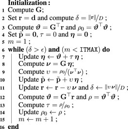
These problems can be overcame by solving the linear system using an iterative method. These methods produce a sequence of vectors that typically converge to the solution at a reasonable rate. The main computational cost associated with these methods is usually some matrix-vector products per iteration. The conjugate gradient (CG) is a very popular iterative method for solving linear systems in equivalent-layer methods. This method was originally developed to solve systems having a square and positive definite matrix. There are two adapted versions of the CG method. The first is called conjugate gradient normal equation residual (CGNR) Golub and Van Loan (2013, Section 11.3) or conjugate gradient least squares (CGLS) (Aster et al., 2019, p. 165) and is used to solve overdetermined problems (Eq. 22). The second is called conjugate gradient normal equation error (CGNE) method Golub and Van Loan (2013), sec. 11.3) and is used to solve the underdetermined problems (Eq. 23). Algorithm 1 outlines the CGLS method applied to the overdetermined problem (Eq. 22).

Algorithm 1. Generic pseudo-code for the CGLS applied to the overdetermined problem (Eq. 22) for the particular case in which H = I_P (Eq. 9; subsection 3.2), μ = 0 (Eq. 11), W_d = I_D (Eq. 12) and $\bar{\mathbf{p}}=\mathbf{0}$ (Eq. 14), where I_P and I_D are the identities of order P and D, respectively.

4 Floating-point operations

Two important factors affecting the efficiency of a given matrix algorithm are the storage and amount of required arithmetic. Here, we quantify this last factor associated with different computational strategies to solve the linear system of the equivalent-layer technique (Section 7). To do it, we opted by counting flops, which are floating point additions, subtractions, multiplications or divisions (Golub and Van Loan, 2013, p. 12–14). This is a non-hardware dependent approach that allows us to do direct comparison between different equivalent-layer methods. Most of the flops count used here can be found in Golub and Van Loan (2013, p. 12, 106, 107 and 164).

Let us consider the case in which the overdetermined problem (Eq. 22) is solved by Cholesky factorization (Eqs. 25, 26) directly for the parameter vector $\tilde{\mathbf{p}}$ by considering the particular case in which H = I_P (Eq. 9; Subsection 3.2), μ = 0 (Eq. 11), W_d = I_D (Eq. 12) and $\bar{\mathbf{p}}=\mathbf{0}$ (Eq. 14), where I_P and I_D are the identities of order P and D, respectively. Based on the information provided in Table 1, the total number of flops can be determined by aggregating the flops required for various computations. These computations include the matrix-matrix and matrix-vector products G^⊤G and G^⊤d, the Cholesky factor $\mathcal{G}$, and the solution of triangular systems. Thus, we can express the total number of flops as follows:

$f_{\mathtt{C}\mathtt{h}\mathtt{o}\mathtt{l}\mathtt{e}\mathtt{s}\mathtt{k}\mathtt{y}}=1/3D^3+2D^2+2\left(P^2+P\right)D.(27)$

The same particular overdetermined problem can be solved by using the CGLS method (Algorithm 1). In this case, we use Table 1 again to combine the total number of flops associated with the matrix-vector and inner products defined in line 3, before starting the iteration, and the 3 saxpys, 2 inner products and 2 matrix-vector products per iteration (lines 7–12). By considering a maximum number of iterations $\mathtt{I}\mathtt{T}\mathtt{M}\mathtt{A}\mathtt{X}$, we obtain

$f_{\mathtt{C}\mathtt{G}\mathtt{L}\mathtt{S}}=2PD+\mathtt{I}\mathtt{T}\mathtt{M}\mathtt{A}\mathtt{X}\left(4PD+4D\right).(28)$

The same approach used to deduce (Eqs. 27, 28) is applied to compute the total number of flops for the selected equivalent-layer methods discussed in Section 7.

TABLE 1

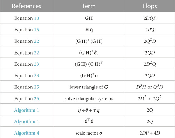
TABLE 1. Total number of flops associated with some useful terms according to Golub and Van Loan (2013, p. 12). The number of flops associated with Eqs. 25, 26 depends if the problem is over or underdetermined. Note that P = Q for the case in which H = I_P (Subsection 3.2). The term η ←ϑ + τ η is a vector update called saxpy (Golub and Van Loan, 2013, p. 4). The terms defined here are references to compute the total number of flops throughout the manuscript.

To simplify our analysis, we do not consider the number of flops required to compute the sensitivity matrix G (Eq. 3) or the matrix A associated with a given potential-field transformation (Eq. 4) because they depend on the specific harmonic functions g_ij and a_ij (Equations 2 and 5). We also neglect the required flops to compute H, W_d, W_q (Eqs. 9, 12 and 13), $\bar{\mathbf{p}}$ (Eq. 14), retrieve $\tilde{\mathbf{q}}$ from ${\tilde{\mathit{\delta }}}_q$ (Eq. 18) and computing δ_d (Eq. 19).

5 Numerical stability

All equivalent-layer methods aim at obtaining an estimate $\tilde{\mathbf{p}}$ for the parameter vector p (Eq. 3), which contains the physical property of the equivalent sources. Some methods do it by first obtaining an estimate $\tilde{\mathbf{q}}$ for the reparameterized parameter vector q (Eq. 9) and then using it to obtain $\tilde{\mathbf{p}}$ (Eq. 15). The stability of a solution $\tilde{\mathbf{p}}$ against noise in the observed data is rarely addressed. Here, we follow the numerical stability analysis presented in Siqueira et al. (2017).

For a given equivalent-layer method (Section 7), we obtain an estimate $\tilde{\mathbf{p}}$ assuming noise-free potential-field data d. Then, we create L different noise-corrupted data d^ℓ, ℓ ∈ {1: L}, by adding L different sequences of pseudorandom Gaussian noise to d, all of them having zero mean. From each d^ℓ, we obtain an estimate ${\tilde{\mathbf{p}}}^{\ell }$. Regardless of the particular equivalent-layer method used, the following inequality (Aster et al., 2019, p. 66) holds true:

$\mathrm{\Delta }{p}^{\ell }\le \kappa \mathrm{\Delta }{d}^{\ell },\ell \in \left\{1:L\right\},(29)$

where κ is the constant of proportionality between the model perturbation

$\mathrm{\Delta }{p}^{\ell }=\frac{\Vert {\tilde{\mathbf{p}}}^{\ell }-\tilde{\mathbf{p}}\Vert }{\Vert \tilde{\mathbf{p}}\Vert },\ell \in \left\{1:L\right\},(30)$

and the data perturbation

$\mathrm{\Delta }{d}^{\ell }=\frac{\Vert {\mathbf{d}}^{\ell }-\mathbf{d}\Vert }{\Vert \mathbf{d}\Vert },\ell \in \left\{1:L\right\},(31)$

with ‖ ⋅‖ representing the Euclidean norm. The constant κ acts as the condition number associated with the pseudo-inverse in a given linear inversion. The larger (smaller) the value of κ, the more unstable (stable) is the estimated solution. Because of that, we designate κ as stability parameter. Equation 29 shows a linear relationship between the model perturbation Δp^ℓ and the data perturbation Δd^ℓ (Eqs. 30 and 31). We estimate the κ (Eq. 29) associated with a given equivalent-layer method as the slope of the straight line fitted to the numerical stability curve formed by the L points $\left(\mathrm{\Delta }{p}^{\ell },\mathrm{\Delta }{d}^{\ell }\right)$.

6 Notation for subvectors and submatrices

Here, we use a notation inspired on that presented by Van Loan (1992, p. 4) to represent subvectors and submatrices. Subvectors of d, for example, are specified by d[i], where i is a list of integer numbers that “pick out” the elements of d forming the subvector d[i]. For example, i = (1, 6, 4, 6) gives the subvector $\mathbf{d}[\mathbf{i}]={[d_1{d}_6{d}_4{d}_6]}^{\top }$. Note that the list i of indices may be sorted or not and it may also have repeated indices. For the particular case in which the list has a single element i = (i), then it can be used to extract the ith element d_i ≡d[i] of d. Sequential lists can be represented by using the colon notation. We consider two types of sequential lists. The first has starting index is smaller than the final index and increment of 1. The second has starting index is greater than the final index and increment of −1. For example,

$\begin{array}{cc}\hfill \mathbf{i}=\left(3:8\right)& \iff \mathbf{d}\left[\mathbf{i}\right]={\left[d_3{d}_4\dots d_8\right]}^{\top }\hfill \\ \hfill \mathbf{i}=\left(8:3\right)& \iff \mathbf{d}\left[\mathbf{i}\right]={\left[d_8{d}_7\dots d_3\right]}^{\top }\hfill \\ \hfill \mathbf{i}=\left(:8\right)& \iff \mathbf{d}\left[\mathbf{i}\right]={\left[d_1{d}_2\dots d_8\right]}^{\top }\hfill \\ \hfill \mathbf{i}=\left(3:\right)& \iff \mathbf{d}\left[\mathbf{i}\right]={\left[d_3{d}_4\dots d_D\right]}^{\top }\hfill \end{array},$

where D is the number of elements forming d.

The notation above can also be used to define submatrices of a D × P matrix G. For example, i = (2, 7, 4, 6) and j = (1, 3, 8) lead to the submatrix

$\mathbf{G}\left[\mathbf{i},\mathbf{j}\right]=\left[\begin{array}{ccc}\hfill g_{21}\hfill & \hfill g_{23}\hfill & \hfill g_{28}\hfill \\ \hfill g_{71}\hfill & \hfill g_{73}\hfill & \hfill g_{78}\hfill \\ \hfill g_{41}\hfill & \hfill g_{43}\hfill & \hfill g_{48}\hfill \\ \hfill g_{61}\hfill & \hfill g_{63}\hfill & \hfill g_{68}\hfill \end{array}\right].$

Note that, in this case, the lists i and j “pick out”, respectively, the rows and columns of G that form the submatrix G[i, j]. The ith row of G is given by the 1 × P vector G[i, :]. Similarly, the D × 1 vector G[:, j] represents the jth column. Finally, we may use the colon notation to define the following submatrix:

$\mathbf{i}=\left(2:5\right),\mathbf{j}=\left(3:7\right)\iff \mathbf{G}\left[\mathbf{i},\mathbf{j}\right]=\left[\begin{array}{ccccc}\hfill g_{23}\hfill & \hfill g_{24}\hfill & \hfill g_{25}\hfill & \hfill g_{26}\hfill & \hfill g_{27}\hfill \\ \hfill g_{33}\hfill & \hfill g_{34}\hfill & \hfill g_{35}\hfill & \hfill g_{36}\hfill & \hfill g_{37}\hfill \\ \hfill g_{43}\hfill & \hfill g_{44}\hfill & \hfill g_{45}\hfill & \hfill g_{46}\hfill & \hfill g_{47}\hfill \\ \hfill g_{53}\hfill & \hfill g_{54}\hfill & \hfill g_{55}\hfill & \hfill g_{56}\hfill & \hfill g_{57}\hfill \end{array}\right],$

which contains the contiguous elements of G from rows 2 to 5 and from columns 3 to 7.

7 Computational strategies

The linear inverse problem of the equivalent-layer technique (Section 3) for the case in which there are large volumes of potential-field data requires dealing with.

(i) the large computer memory to store large and full matrices;

(ii) the long computation time to multiply a matrix by a vector; and

(iii) the long computation time to solve a large linear system of equations.

Here, we review some strategies aiming at reducing the computational cost of the equivalent-layer technique. We quantify the computational cost by using flops (Section 4) and compare the results with those obtained for Cholesky factorization and CGLS (Eqs. 27, 28). We focus on the overall strategies used by the selected methods.

7.1 Moving window

The initial approach to enhance the computational efficiency of the equivalent-layer technique is commonly denoted moving window and involves first splitting the observed data d_i, i ∈ {1: D}, into M overlapping subsets (or data windows) formed by D^m data each, m ∈ {1: M}. The data inside the mth window are usually adjacent to each other and have indices defined by an integer list i^m having D^m elements. The number of data D^m forming the data windows are not necessarily equal to each other. Each data window has a D^m × 1 observed data vector d^m ≡d[i^m]. The second step consists in defining a set of P equivalent sources with scalar physical property p_j, j ∈ {1: P}, and also split them into M overlapping subsets (or source windows) formed by P^m data each, m ∈ {1: M}. The sources inside the mth window have indices defined by an integer list j^m having P^m elements. Each source window has a P^m × 1 parameter vector p^m and is located right below the corresponding mth data window. Then, each d^m ≡d[i^m] is approximated by

${\mathbf{f}}^m={\mathbf{G}}^m{\mathbf{p}}^m,(32)$

where G^m ≡G[i^m, j^m] is a submatrix of G (Eq. 3) formed by the elements computed with Eq. 2 using only the data and equivalent sources located inside the window mth. The main idea of the moving-window approach is using the ${\tilde{\mathbf{p}}}^m$ estimated for each window to obtain 1) an estimate $\tilde{\mathbf{p}}$ of the parameter vector for the entire equivalent layer or 2) a given potential-field transformation t (Eq. 4). The main advantages of this approach is that 1) the estimated parameter vector $\tilde{\mathbf{p}}$ or transformed potential field are not obtained by solving the full, but smaller linear systems and 2) the full matrix G (Eq. 3) is never stored.

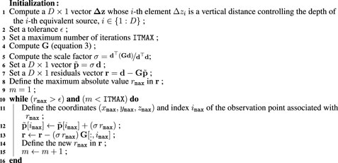
Leão and Silva (1989) presented a pioneer work using the moving-window approach. Their method requires a regularly-spaced grid of observed data on a horizontal plane z₀. The data windows are defined by square local grids of $\sqrt{D^{\prime }}\times \sqrt{D^{\prime }}$ adjacent points, all of them having the same number of points D′. The equivalent sources in the mth data window are located below the observation plane, at a constant vertical distance Δz₀. They are arranged on a regular grid of $\sqrt{P^{\prime }}\times \sqrt{P^{\prime }}$ adjacent points following the same grid pattern of the observed data. The local grid of sources for all data windows have the same number of elements P′. Besides, they are vertically aligned, but expands the limits of their corresponding data windows, so that D′ < P′. Because of this spatial configuration of observed data and equivalent sources, we have that G^m = G′ Eq. 32 for all data windows (i.e., ∀ m ∈ {1: M}), where G′ is a D′ × P′ constant matrix.

By omitting the normalization strategy used by Leão and Silva (1989), their method consists in directly computing the transformed potential field $t_c^m$ at the central point $(x_c^m,y_c^m,z_0+\mathrm{\Delta }{z}_0)$ of each data window as follows:

$t_c^m={\left({\mathbf{a}}^{\prime }\right)}^{\top }{\mathbf{B}}^{\prime }{\mathbf{d}}^m,m\in \left\{1:M\right\},(33)$

where a′ is a P′ × 1 vector with elements computed by Eq. 5 by using all equivalent sources in the mth window and only the coordinate of the central point in the mth data window and

${\mathbf{B}}^{\prime }={\left({\mathbf{G}}^{\prime }\right)}^{\top }{\left[{\mathbf{G}}^{\prime }{\left({\mathbf{G}}^{\prime }\right)}^{\top }+\mu {\mathbf{I}}_{D^{\prime }}\right]}^{-1}(34)$

is a particular case of matrix B associated with underdetermined problems Eq. 21 for the particular case in which H = W_q = I_P′ (Eqs. 9, 13), W_d = I_D′ (Eq. 12), $\bar{\mathbf{p}}=\mathbf{0}$ (Eq. 14), where I_P′ and I_D′ are identity matrices of order P′ and D′, respectively, and 0 is a vector of zeros. Due to the presumed spatial configuration of the observed data and equivalent sources, a′ and G′ are the same for all data windows. Hence, only the data vector d^m is modified according to the position of the data window. Note that Eq. 33 combines the potential-field transformation (Eq. 4) with the solution of the undetermined problem (Eq. 23).

The method proposed by Leão and Silva (1989) can be outlined by the Algorithm 2. Note that Leão and Silva (1989) directly compute the transformed potential $t_c^m$ at the central point of each data window without explicitly computing and storing an estimated for p^m (Eq. 32). It means that their method allows computing a single potential-field transformation. A different transformation or the same one evaluated at different points require running their moving-data window method again.

Algorithm 2. Generic pseudo-code for the method proposed by Leão and Silva (1989).

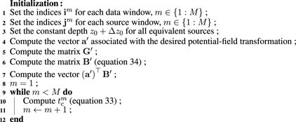
The total number of flops in Algorithm 2 depends on computing the P′ × D′ matrix B′ (Eq. 34) in line 6 and use it to define the 1 × P′ vector ${\left({\mathbf{a}}^{\prime }\right)}^{\top }{\mathbf{B}}^{\prime }$ (line 7) before starting the iterations and computing an inner product (Eq. 33) per iteration. We consider that the total number of flops associated with B′ is obtained by the matrix-matrix product ${\mathbf{G}}^{\prime }{\left({\mathbf{G}}^{\prime }\right)}^{\top }$, its inverse and then the premultiplication by ${\left({\mathbf{G}}^{\prime }\right)}^{\top }$. By using Table 1 and considering that inverse is computed via Cholesky factorization, we obtain that the total number of flops for lines 6 and 7 is 2(D′)²P′ + 7(D′)³/6 + 2(D′)²P′. Then, the total number of flops for Algorithm 2 is

$f_{\mathtt{L}\mathtt{S}\mathtt{8}\mathtt{9}}=7/6{\left(D^{\prime }\right)}^3+4P^{\prime }{\left(D^{\prime }\right)}^2+M2P^{\prime }.(35)$

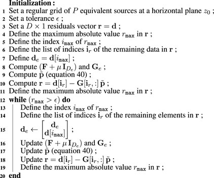
Soler and Uieda (2021) generalized the method proposed by Leão and Silva (1989) for irregularly spaced data on an undulating surface. A direct consequence of this generalization is that a different submatrix G^m ≡G[i^m, j^m] (Eq. 32) must be computed for each window. Differently from Leão and Silva (1989), Soler and Uieda (2021) store the computed ${\tilde{\mathbf{p}}}^m$ for all windows and subsequently use them to obtain a desired potential-field transformation (Eq. 4) as the superposed effect of all windows. The estimated ${\tilde{\mathbf{p}}}^m$ for all windows are combined to form a single P × 1 vector $\tilde{\mathbf{p}}$, which is an estimate for original parameter vector p (Eq. 3). For each data window, Soler and Uieda (2021) solve an overdetermined problem (Eq. 22) for ${\tilde{\mathbf{p}}}^m$ by using $\mathbf{H}={\mathbf{W}}_q={\mathbf{I}}_{P^m}$ (Eqs. 9, 13), ${\mathbf{W}}_d^m$ (Eq. 12) equal to a diagonal matrix of weights for the data inside the mth window and $\bar{p}=\mathbf{0}$ (Eq. 14), so that

$\left[{\left({\mathbf{G}}^m\right)}^{\top }{\mathbf{W}}_d^m{\mathbf{G}}^m+\mu {\mathbf{I}}_{P^{\prime }}\right]{\tilde{\mathbf{p}}}^m={\left({\mathbf{G}}^m\right)}^{\top }{\mathbf{W}}_d^m{\mathbf{d}}^m.(36)$

Unlike Leão and Silva (1989), Soler and Uieda (2021) do not adopt a sequential order of the data windows; rather, they adopt a randomized order of windows in their iterations. The overall steps of the method proposed by Soler and Uieda (2021) are defined by the Algorithm 3. For convenience, we have omitted the details about the randomized window order, normalization strategy employed and block-averaged sources layout proposed by those authors (see Subsection 2.1). Note that this algorithm starts with a residuals vector r that is iteratively updated. The iterative algorithm in Soler and Uieda (2021) estimates a solution (${\tilde{\mathbf{p}}}^m$ in Eq. 36 using the data and the equivalent sources that fall within a moving-data window; however, it calculates the predicted data and the residual data in the whole survey data. Next, the residual data that fall within a new position of the data window is used as input data to estimate a new solution within the data window which, in turn, is used to calculated a new predicted data and a new residual data in the whole survey data.

Algorithm 3. Generic pseudo-code for the method proposed by Soler and Uieda (2021).

The computational cost of Algorithm 3 can be defined in terms of the linear system (Eq. 36) to be solved for each window (line 10) and the subsequent updates in lines 11 and 12. We consider that the linear system cost can be quantified by the matrix-matrix and matrix-vector products ${\left({\mathbf{G}}^m\right)}^{\top }{\mathbf{G}}^m$ and ${\left({\mathbf{G}}^m\right)}^{\top }{\mathbf{d}}^m$, respectively, and solution of the linear system (line 10) via Cholesky factorization (Eqs. 25, 26). The following updates represent a saxpy without scalar-vector product (line 11) and a matrix-vector product (line 12). In this case, according to Table 1, the total number of flops associated with Algorithm 3 is given by:

$f_{\mathtt{S}\mathtt{U}\mathtt{2}\mathtt{1}}=M\left[1/3{\left(P^{\prime }\right)}^3+2\left(D^{\prime }\right){\left(P^{\prime }\right)}^2+\left(4D^{\prime }\right)P^{\prime }\right],(37)$

where P′ and D′ represent, respectively, the average number of equivalent sources and data at each window.

7.2 Column-action update

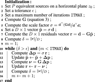
Cordell (1992) proposed a column-action update strategy similar to those applied to image reconstruction methods (e.g., Elfving et al., 2017). His approach, that was later used by Guspí and Novara (2009), relies on first defining one equivalent source located right below each observed data d_i, i ∈ {1: D}, at a vertical coordinate z_i + Δz_i, where Δz_i is proportional to the distance from the ith observation point (x_i, y_i, z_i) to its closest neighbor. The second step consists in updating the physical property p_j of a single equivalent source, j ∈ {1: D} and remove its predicted potential field from the observed data vector d, producing a residuals vector r. At each iteration, the single equivalent source is the one located vertically beneath the observation station of the maximum data residual. Next, the predicted data produced by this single source is calculated over all of the observation points and a new data residual r and the D × 1 parameter vector p containing the physical property of all equivalent sources are updated iteratively. During each subsequent iteration, Cordell’s method either incorporates a single equivalent source or adjusts an existing equivalent source to match the maximum amplitude of the current residual field. The convergence occurs when all of the residuals are bounded by an envelope of prespecified expected error. At the end, the algorithm produces an estimate $\tilde{\mathbf{p}}$ for the parameter vector yielding a predicted potential field f (Eq. 3) satisfactorily fitting the observed data d according to a given criterion. Note that the method proposed by Cordell (1992) iteratively solves the linear $\mathbf{G}\tilde{\mathbf{p}}\approx \mathbf{d}$ with a D × D matrix G. At each iteration, only a single column of G (Eq. 3) is used. An advantage of this column-action update approach is that the full matrix G is never stored.

Algorithm 4 delineates the Cordell’s method. We have introduced a scale factor σ to improve convergence. Note that a single column $\mathbf{G}[:,i_{\max }]$ of the D × D matrix G (Eq. 3) is used per iteration, where $i_{\max }$ is the index of the maximum absolute value in r. As pointed out by Cordell (1992), the method does not necessarily decrease monotonically along the iterations. Besides, the method may not converge depending on how the vertical distances Δz_i, i ∈ {1: D}, controlling the depths of the equivalent sources are set. According to Cordell (1992), the maximum absolute value $r_{\max }$ in r decreases robustly at the beginning and oscillates within a narrowing envelope for the subsequent iterations.

Algorithm 4. Generic pseudo-code for the method proposed by Cordell (1992).

Guspí and Novara (2009) generalized Cordell’s method to perform reduction to the pole and other transformations on scattered magnetic observations by using two steps. The first step involves computing the vertical component of the observed field using equivalent sources while preserving the magnetization direction. In the second step, the vertical observation direction is maintained, but the magnetization direction is shifted to the vertical. The main idea employed by both Cordell (1992) and Guspí and Novara (2009) is an iterative scheme that uses a single equivalent source positioned below a measurement station to compute both the predicted data and residual data for all stations. This approach entails a computational strategy where a single column of the sensitivity matrix G (Eq. 3) is calculated per iteration.

The total number of flops in Algorithm 4 consists in computing the scale factor σ (line 5), computing an initial approximation for the parameter vector and the residuals (lines 6 and 7) and finding the maximum absolute value in vector r (line 8) before the while loop. Per iteration, there is a saxpy (line 13) and another search for the maximum absolute value in vector r (line 14). By considering that selecting the maximum absolute value in a D × 1 vector is a D log₂(D) operation (e.g., Press et al., 2007, p. 420), we get from Table 1 that the total number of flops in Algorithm 38 is given by:

$f_{\mathtt{C}\mathtt{9}\mathtt{2}}=4D^2+6D+D{\log }_2\left(D\right)+\mathtt{I}\mathtt{T}\mathtt{M}\mathtt{A}\mathtt{X}\left[2D+D{\log }_2\left(D\right)\right].(38)$

7.3 Row-action update

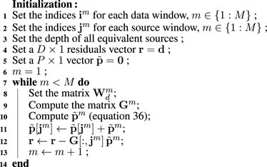
To reduce the total processing time and memory usage of equivalent-layer technique, Mendonça and Silva (1994) proposed a strategy called equivalent data concept. The equivalent data concept is grounded on the principle that there is a subset of redundant data that does not contribute to the final solution and thus can be dispensed. Conversely, there is a subset of observations, called equivalent data, that contributes effectively to the final solution and fits the remaining observations (redundant data). Iteratively, Mendonça and Silva (1994) selected the subset of equivalent data that is substantially smaller than the original dataset. This selection is carried out by incorporating one data point at a time.

The method presented by Mendonça and Silva (1994) is a type of algebraic reconstruction technique (ART) (e.g., van der Sluis and van der Vorst, 1987, p. 58) or row-action update (e.g., Elfving et al., 2017) to estimate a parameter vector $\tilde{\mathbf{p}}$ for a regular grid of P equivalent sources on a horizontal plane z₀. Such methods iterate on the linear system rows to estimate corrections for the parameter vector, which may substantially save computer time and memory required to compute and store the full linear system matrix along the iterations. The convergence of such methods strongly depends on the linear system condition. The main advantage of such methods is not computing and storing the full linear system matrix, but iteratively using its rows. In contrast to common row-action algorithms, the rows in Mendonça and Silva (1994) are not processed sequentially. Instead, in Mendonça and Silva (1994), the rows are introduced according to their residual magnitudes (maximum absolute value in r), which are computed based on the estimate over the equivalent layer from the previous iteration. The particular row-action method proposed by Mendonça and Silva (1994) considers that

$\mathbf{d}=\left[\begin{array}{c}\hfill {\mathbf{d}}_e\hfill \\ \hfill {\mathbf{d}}_r\hfill \end{array}\right],\mathbf{G}=\left[\begin{array}{c}\hfill {\mathbf{G}}_e\hfill \\ \hfill {\mathbf{R}}_r\hfill \end{array}\right],(39)$

where d_e and d_r are D_e × 1 and D_r × 1 vectors and G_e and G_r are D_e × P and D_r × P matrices, respectively. Mendonça and Silva (1994) designate d_e and d_r as, respectively, equivalent and redundant data. With the exception of a normalization strategy, Mendonça and Silva (1994) calculate a P × 1 estimated parameter vector $\tilde{\mathbf{p}}$ by solving an underdetermined problem (Eq. 23) involving only the equivalent data d_e (Eq. 39) for the particular case in which H = W_p = I_P (Eqs. 9, 13), ${\mathbf{W}}_d={\mathbf{I}}_{D_e}$ (Eq. 12) and $\bar{p}=\mathbf{0}$ (Eq. 14), which results in

$\begin{array}{c}\hfill \left(\mathbf{F}+\mu {\mathbf{I}}_{D_e}\right)\mathbf{u}={\mathbf{d}}_e\\ \hfill \tilde{\mathbf{p}}={\mathbf{G}}_e^{\top }\mathbf{u}\end{array},(40)$

where F is a computationally-efficient D_e × D_e matrix that approximates ${\mathbf{G}}_e{\mathbf{G}}_e^{\top }$. Mendonça and Silva (1994) presume that the estimated parameter vector $\tilde{\mathbf{p}}$ obtained from Eq. 40 leads to a D_r × 1 residuals vector

$\mathbf{r}={\mathbf{d}}_r-{\mathbf{G}}_r\tilde{\mathbf{p}}(41)$

having a maximum absolute value $r_{\max }\le ϵ$, where ϵ is a predefined tolerance.

The overall method of Mendonça and Silva (1994) is defined by Algorithm 5. It is important noting that the number D_e of equivalent data in d_e increases by one per iteration, which means that the order of the linear system in Eq. 40 also increases by one at each iteration. Those authors also propose a computational strategy based on Cholesky factorization (e.g., Golub and Van Loan, 2013, p. 163) for efficiently updating $\left(\mathbf{F}+\mu {\mathbf{I}}_{D_e}\right)$ at a given iteration (line 16 in Algorithm 5) by computing only its new elements with respect to those computed in the previous iteration.

Algorithm 5. Generic pseudo-code for the method proposed by Mendonça and Silva (1994).

7.4 Reparameterization

Another approach for improving the computational performance of equivalent-layer technique consists in setting a P × Q reparameterization matrix H (Eq. 9) with Q ≪ P. This strategy has been used in applied geophysics for decades (e.g., Skilling and Bryan, 1984; Kennett et al., 1988; Oldenburg et al., 1993; Barbosa et al., 1997) and is known as subspace method. The main idea relies in reducing the linear system dimension from the original P-space to a lower-dimensional subspace (the Q-space). An estimate $\tilde{\mathbf{q}}$ for the reparameterized parameter vector q is obtained in the Q-space and subsequently used to obtain an estimate $\tilde{\mathbf{p}}$ for the parameter vector p (Eq. 3) in the P-space by using Eq. 9. Hence, the key aspect of this reparameterization approach is solving an appreciably smaller linear inverse problem for $\tilde{\mathbf{q}}$ than that for the original parameter vector $\tilde{\mathbf{p}}$ (Eq. 3).

Oliveira Jr. et al. (2013) have used this approach to describe the physical property distribution on the equivalent layer in terms of piecewise bivariate polynomials. Specifically, their method consists in splitting a regular grid of equivalent sources into source windows inside which the physical-property distribution is described by bivariate polynomial functions. The key aspect of their method relies on the fact that the total number of coefficients required to define the bivariate polynomials is considerably smaller than the original number of equivalent sources. Hence, they formulate a linear inverse problem for estimating the polynomial coefficients and use them later to compute the physical property distribution on the equivalent layer.

The method proposed by Oliveira Jr. et al. (2013) consists in solving an overdetermined problem (Eq. 22) for estimating the polynomial coefficients $\tilde{\mathbf{q}}$ with W_d = I_D (Eq. 12) and $\bar{q}=\mathbf{0}$ (Eq. 14), so that

$\left({\mathbf{H}}^{\top }{\mathbf{G}}^{\top }\mathbf{G}\mathbf{H}+\mu {\mathbf{W}}_q\right)\tilde{\mathbf{q}}={\mathbf{H}}^{\top }{\mathbf{G}}^{\top }\mathbf{d},(42)$

where W_q = H^⊤W_p H is defined by a matrix W_p representing the zeroth- and first-order Tikhonov regularization (e.g., Aster et al., 2019, p. 103). Note that, in this case, the prior information is defined in the P-space for the original parameter vector p and then transformed to the Q-space. Another characteristic of their method is that it is valid for processing irregularly-spaced data on an undulating surface.

Mendonça (2020) also proposed a reparameterization approach for the equivalent-layer technique. Their approach, however, consists in setting H as a truncated singular value decomposition (SVD) (e.g., Aster et al., 2019, p. 55) of the observed potential field. Differently from Oliveira Jr. et al. (2013), however, the method of Mendonça (2020) requires a regular grid of potential-field data on horizontal plane. Another difference is that these authors uses W_q = I_Q (Eq. 13), which means that the regularization is defined directly in the Q-space.

We consider an algorithm (not shown) that solves the overdetermined problem (Eq. 22) by combining the reparameterization with CGLS method (Algorithm 1). It starts with a reparameterization step defined by defining a matrix C = G H (Eq. 10). Then, the CGLS (Algorithm 1) is applied by replacing G with C. In this case, the linear system is solved by the reparameterized parameter vector $\tilde{\mathbf{q}}$ instead of $\tilde{\mathbf{p}}$. At the end, the estimated $\tilde{\mathbf{q}}$ is transformed into $\tilde{\mathbf{p}}$ (Eq. 15). Compared to the original CGLS shown in Algorithm 1, the algorithm discussed here has the additional flops associated with the matrix-matrix product to compute C and the matrix-vector product of Eq. 15 outside the while loop. Then, according to Table 1, the total number of flops given by:

$f_{\mathtt{r}\mathtt{e}\mathtt{p}\mathtt{a}\mathtt{r}\mathtt{a}\mathtt{m}.}=2Q\left(DP+D\right)+2PQ+\mathtt{I}\mathtt{T}\mathtt{M}\mathtt{A}\mathtt{X}\left(4QD+4D\right).(43)$

The important aspect of this approach is that, for the case in which Q ≪ P (Eq. 9), the number of flops per iteration can be substantially decreased with respect to those associated with Algorithm 1. In this case, the flops decrease per iteration compensates the additional flops required to compute C and obtain $\tilde{\mathbf{p}}$ from $\tilde{\mathbf{q}}$ (Eq. 15).

7.5 Sparsity induction

Li and Oldenburg (2010) proposed a method that applies the discrete wavelet transform to introduce sparsity into the original dense matrix G (Eq. 3). Those authors approximate a planar grid of potential-field data by a regularly-spaced grid of equivalent sources, so that the number of data D and sources P is the same, i.e., D = P. Specifically, Li and Oldenburg (2010) proposed a method that applies the wavelet transform to the original dense matrix G and sets to zero the small coefficients that are below a given threshold, which results in an approximating sparse representation of G in the wavelet domain. They first consider the following approximation

${\mathbf{d}}_w\approx {\mathbf{G}}_s{\mathbf{p}}_w,(44)$

where

${\mathbf{d}}_w=\mathcal{W}\mathbf{d},{\mathbf{p}}_w=\mathcal{W}\mathbf{p},(45)$

are the observed data and parameter vector in the wavelet domain; $\mathcal{W}$ is a D × D orthogonal matrix defining a discrete wavelet transform; and G_s is a sparse matrix obtained by setting to zero the elements of

${\mathbf{G}}_w=\mathcal{W}\mathbf{G}{\mathcal{W}}^{\top }(46)$

with absolute value smaller than a given threshold.

Li and Oldenburg (2010) solve a normalized inverse problem in the wavelet domain. Specifically, they first define a matrix

${\mathbf{G}}_L={\mathbf{G}}_s{\mathbf{L}}^{-1}(47)$

and a normalized parameter vector

${\mathbf{p}}_L=\mathbf{L}{\mathbf{p}}_w,(48)$

where L is a diagonal and invertible matrix representing an approximation of the first-order Tikhonov regularization in the wavelet domain. Then they solve an overdetermined problem (Eq. 22) to obtain an estimate ${\tilde{\mathbf{p}}}_L$ for p_L (Eq. 48), with G_L (Eq. 47), H = I_P (Eq. 9), μ = 0 (Eq. 11), W_d = I_D (Eq. 12) and $\bar{p}=\mathbf{0}$ (Eq. 14) via conjugate-gradient method (e.g., Golub and Van Loan, 2013; Section 11.3). Finally, Li and Oldenburg (2010) compute an estimate $\tilde{\mathbf{p}}$ for the original parameter vector given by

$\tilde{\mathbf{p}}={\mathcal{W}}^{\top }\left({\mathbf{L}}^{-1}{\tilde{\mathbf{p}}}_L\right),(49)$

where the term within parenthesis is an estimate ${\tilde{\mathbf{p}}}_w$ of the parameter vector p_w (Eq. 45) in the wavelet domain and matrix ${\mathcal{W}}^{\top }$ represents an inverse wavelet transform.

Barnes and Lumley (2011) also proposed a computationally efficient method for equivalent-layer technique by inducing sparsity into the original sensitivity matrix G (Eq. 3). Their approach consists in setting a P × Q reparameterization matrix H (Eq. 9) with Q ≈ 1.7 P. Note that, differently from Oliveira Jr. et al. (2013) and Mendonça (2020), Barnes and Lumley (2011) do not use the reparameterization with the purpose of reducing the number of the parameters. Instead, they use a reparameterization scheme that groups distant equivalent sources into blocks by using a bisection process. This scheme leads to a quadtree representation of the physical-property distribution on the equivalent layer, so that matrix GH (Eq. 10) is notably sparse. Barnes and Lumley (2011) explore this sparsity in solving the overdetermined problem for $\tilde{\mathbf{q}}$ (Eq. 42) via conjugate-gradient method (e.g., Golub and Van Loan, 2013; sec. 11.3).

It is difficult to predict the exact sparsity obtained from the methods proposed by Li and Oldenburg (2010) and Barnes and Lumley (2011) because it depends on several factors, including the observed potential-field data. According to Li and Oldenburg (2010), their wavelet approach results in a sparse matrix having $\approx 2\%$ of the elements in G_w (Eq. 46). The reparameterization proposed by Barnes and Lumley (2011) leads to a sparse matrix G H (Eq. 10) with only $\approx 1\%$ of non-zero elements. These sparsity patterns can be efficiently explored, for example, in computing the required matrix-vector products along the iterations of the CGLS method (Algorithm 1).

7.6 Iterative methods using the full matrix $\mathbf{G}$

Xia and Sprowl (1991) introduced an iterative method for estimating the parameter vector $\tilde{\mathbf{p}}$ (Eq. 3), which was subsequently adapted to the Fourier domain by Xia et al. (1993). Their method uses the full and dense sensitivity matrix G (Eq. 3) (without applying any compression or reparameterization, for example,) to compute the predicted data at all observation points per iteration. More than two decades later, Siqueira et al. (2017) have proposed an iterative method similar to that presented by Xia and Sprowl (1991). The difference is that Siqueira et al.’s algorithm was deduced from the Gauss’ theorem (e.g., Kellogg, 1967, p. 43) and the total excess of mass (e.g., Blakely, 1996, p. 60). Besides, Siqueira et al. (2017) have included a numerical analysis showing that their method produces very stable solutions, even for noise-corrupted potential-field data.

The iterative method proposed by Siqueira et al. (2017) is outlined in Algorithm 6, presumes an equivalent layer formed by monopoles (point masses) and can be applied to irregularly-spaced data on an undulating surface. Instead of using the element of area originally proposed by Siqueira et al. (2017), we introduce the scale factor σ, which can be automatically computed from the observed potential-field data. Note that the residuals r are used to compute a correction Δp for the parameter vector at each iteration (line 11), which requires a matrix-vector product involving the full matrix G. Interestingly, this approach for estimating the physical property distribution on an equivalent layer is the same originally proposed by Bott (1960) for estimating the basement relief under sedimentary basins. The methods of Xia and Sprowl (1991) and Siqueira et al. (2017) were originally proposed for processing gravity data, but can be potentially applied to any harmonic function because they actually represent iterative solutions of the classical Dirichlet’s problem or the first boundary value problem of potential theory (Kellogg, 1967, p. 236) on a plane.

Algorithm 6. Generic pseudo-code for the iterative method proposed by Siqueira et al. (2017).

Recently, Jirigalatu and Ebbing (2019) presented another iterative method for estimating a parameter vector $\tilde{\mathbf{p}}$ (Eq. 3). With the purpose of combining different potential-field data, their method basically modifies that shown in Algorithm 6 by changing the initial approximation and the iterative correction for the parameter vector. Specifically, Jirigalatu and Ebbing (2019) replace line 5 by $\tilde{\mathbf{p}}=\mathbf{0}$, where 0 is a vector of zeros, and line 11 by Δp = ω G^⊤r, where ω is a positive scalar defined by trial and error. Note that this modified approach requires two matrix-vector products involving the full matrix G per iteration. To overcome the high computational cost of these two products, Jirigalatu and Ebbing (2019) set an equivalent layer formed by prisms and compute their predicted potential field in the wavenumber domain by using the Gauss-FFT technique Zhao et al. (2018).

The iterative method proposed by Siqueira et al. (2017) (Algorithm 6) requires computing the scale factor σ (line 5), computing an initial approximation for the parameter vector and the residuals (lines 6 and 7) before the main loop. Inside the main loop, there is a half saxpy (lines 11 and 12) to update the parameter vector, a matrix-vector product (line 13) and the residuals update (line 14). Then, we get from Table 1 that the total number of flops is given by:

$f_{\mathtt{S}\mathtt{O}\mathtt{B}\mathtt{1}\mathtt{7}}=4D^2+6D+\mathtt{I}\mathtt{T}\mathtt{M}\mathtt{A}\mathtt{X}\left(2D^2+3D\right).(50)$

Note that the number of flops per iteration in $f_{\mathtt{S}\mathtt{O}\mathtt{B}\mathtt{1}\mathtt{7}}$ (Eq. 50) has the same order of magnitude, but is smaller than that in $f_{\mathtt{C}\mathtt{G}\mathtt{L}\mathtt{S}}$ (Eq. 28).

7.7 Iterative deconvolution

Recently, Takahashi et al. (2020, 2022) proposed the convolutional equivalent-layer method, which explores the structure of the sensitivity matrix G (Eq. 3) for the particular case in which 1) there is a single equivalent source right below each potential-field datum and 2) both data and sources rely on planar and regularly spaced grids. Specifically, they consider a regular grid of D potential-field data at points (x_i, y_i, z₀), i ∈ {1: D}, on a horizontal plane z₀. The data indices i may be ordered along the x − or y − direction, which results in an x − or y − oriented grid, respectively. They also consider a single equivalent source located right below each datum, at a constant vertical coordinate z₀ + Δz, Δz > 0. In this case, the number of data and equivalent sources are equal to each other (i.e., D = P) and G (Eq. 3) assumes a doubly block Toeplitz (Jain, 1989, p. 28) or block-Toeplitz Toeplitz-block (BTTB) (Chan and Jin, 2007, p. 67) structure formed by N_B × N_B blocks, where each block has N_b × N_b elements, with D = N_B N_b. This particular structure allows formulating the product of G and an arbitrary vector as a fast discrete convolution via Fast Fourier Transform (FFT) (Van Loan, 1992; Section 4.2).

Consider, for example, the particular case in which N_B = 4, N_b = 3 and D = 12. In this case, G (Eq. 3) is a 12 × 12 block matrix given by

$\mathbf{G}={\left[\begin{array}{cccc}\hfill {\mathbf{G}}^0\hfill & \hfill {\mathbf{G}}^1\hfill & \hfill {\mathbf{G}}^2\hfill & \hfill {\mathbf{G}}^3\hfill \\ \hfill {\mathbf{G}}^{-1}\hfill & \hfill {\mathbf{G}}^0\hfill & \hfill {\mathbf{G}}^1\hfill & \hfill {\mathbf{G}}^2\hfill \\ \hfill {\mathbf{G}}^{-2}\hfill & \hfill {\mathbf{G}}^{-1}\hfill & \hfill {\mathbf{G}}^0\hfill & \hfill {\mathbf{G}}^1\hfill \\ \hfill {\mathbf{G}}^{-3}\hfill & \hfill {\mathbf{G}}^{-2}\hfill & \hfill {\mathbf{G}}^{-1}\hfill & \hfill {\mathbf{G}}^0\hfill \end{array}\right]}_{D\times D},(51)$

where each block Gⁿ, n ∈ {(1 − N_B): (N_B − 1)}, is a 3 × 3 Toeplitz matrix. Takahashi et al. (2020, 2022) have deduced the specific relationship between blocks Gⁿ and G⁻ⁿ and also between a given block Gⁿ and its transposed ${\left({\mathbf{G}}^n\right)}^{\top }$ according to the harmonic function g_ij (Eq. 2) defining the element ij of the sensitivity matrix G (Eq. 3) and the orientation of the data grid.

Consider the matrix-vector products

$\mathbf{G}\mathbf{v}=\mathbf{w}(52)$

and

${\mathbf{G}}^{\top }\mathbf{v}=\mathbf{w},(53)$

involving a D × D sensitivity matrix G (Eq. 3) defined in terms of a given harmonic function g_ij (Eq. 2), where

$\mathbf{v}={\left[\begin{array}{c}\hfill {\mathbf{v}}^0\hfill \\ \hfill ⋮\hfill \\ \hfill {\mathbf{v}}^{N_B-1}\hfill \end{array}\right]}_{D\times 1},\mathbf{w}={\left[\begin{array}{c}\hfill {\mathbf{w}}^0\hfill \\ \hfill ⋮\hfill \\ \hfill {\mathbf{w}}^{N_B-1}\hfill \end{array}\right]}_{D\times 1},(54)$

are arbitrary partitioned vectors formed by N_B sub-vectors vⁿ and wⁿ, n ∈ {0: (N_B − 1)}, all of them having N_b elements. Eqs. 52, 53 can be computed in terms of an auxiliary matrix-vector product

${\mathbf{G}}_c{\mathbf{v}}_c={\mathbf{w}}_c,(55)$

where

${\mathbf{v}}_c={\left[\begin{array}{c}\hfill {\mathbf{v}}_c^0\hfill \\ \hfill ⋮\hfill \\ \hfill {\mathbf{v}}_c^{N_B-1}\hfill \\ \hfill \mathbf{0}\hfill \end{array}\right]}_{4D\times 1},{\mathbf{w}}_c={\left[\begin{array}{c}\hfill {\mathbf{w}}_c^0\hfill \\ \hfill ⋮\hfill \\ \hfill {\mathbf{w}}_c^{N_B-1}\hfill \\ \hfill \mathbf{0}\hfill \end{array}\right]}_{4D\times 1},(56)$

are partitioned vectors formed by 2N_b × 1 sub-vectors

${\mathbf{v}}_c^n={\left[\begin{array}{c}\hfill {\mathbf{v}}^n\hfill \\ \hfill \mathbf{0}\hfill \end{array}\right]}_{2N_b\times 1},{\mathbf{w}}_c^n={\left[\begin{array}{c}\hfill {\mathbf{w}}^n\hfill \\ \hfill \mathbf{0}\hfill \end{array}\right]}_{2N_b\times 1},(57)$

and G_c is a 4D × 4D doubly block circulant (Jain, 1989, p. 28) or block-circulant circulant-block (BCCB) (Chan and Jin, 2007, p. 76) matrix. What follows aims at explaining how the original matrix-vector products defined by Eqs. 52, 53, involving a D × D BTTB matrix G exemplified by Eq. 51, can be efficiently computed in terms of the auxiliary matrix-vector product given by Eq. 55, which has a 4D × 4D BCCB matrix G_c.

Matrix G_c (Eq. 55) is formed by 2N_B × 2N_B blocks, where each block ${\mathbf{G}}_c^n$, n ∈ {(1 − N_B): (N_B − 1)} is a 2N_b × 2N_b circulant matrix. For the case in which the original matrix-vector product is that defined by Eq. 52, the first column of blocks forming the BCCB matrix G_c is given by

${\mathbf{G}}_c\left[:,:2N_b\right]={\left[\begin{array}{c}\hfill {\mathbf{G}}_c^0\hfill \\ \hfill {\mathbf{G}}_c^{-1}\hfill \\ \hfill ⋮\hfill \\ \hfill {\mathbf{G}}_c^{1-N_B}\hfill \\ \hfill \mathbf{0}\hfill \\ \hfill {\mathbf{G}}_c^{N_B-1}\hfill \\ \hfill ⋮\hfill \\ \hfill {\mathbf{G}}_c^1\hfill \end{array}\right]}_{4D\times 2N_b},(58)$

with blocks ${\mathbf{G}}_c^n$ having the first column given by

$\begin{array}{ll}\hfill {\mathbf{G}}_c^n\left[:,1\right]& ={\left[\begin{array}{c}\hfill {\mathbf{G}}^n\left[:,1\right]\hfill \\ \hfill 0\hfill \\ \hfill {\left({\mathbf{G}}^n\left[1,N_b:2\right]\right)}^{\top }\hfill \end{array}\right]}_{2N_b\times 2N_b},\hfill \\ \hfill & n\in \left\{\left(1-N_B\right):\left(N_B-1\right)\right\},\hfill \end{array}(59)$

where Gⁿ are the blocks forming the BTTB matrix G (Eq. 51). For the case in which the original matrix-vector product is that defined by Eq. 53, the first column of blocks forming the BCCB matrix G_c is given by

${\mathbf{G}}_c\left[:,:2N_b\right]={\left[\begin{array}{c}\hfill {\mathbf{G}}_c^0\hfill \\ \hfill {\mathbf{G}}_c^1\hfill \\ \hfill ⋮\hfill \\ \hfill {\mathbf{G}}_c^{N_B-1}\hfill \\ \hfill \mathbf{0}\hfill \\ \hfill {\mathbf{G}}_c^{1-N_B}\hfill \\ \hfill ⋮\hfill \\ \hfill {\mathbf{G}}_c^{-1}\hfill \end{array}\right]}_{4D\times 2N_b},(60)$

with blocks ${\mathbf{G}}_c^n$ having the first column given by

${\mathbf{G}}_c^n\left[:,1\right]={\left[\begin{array}{c}\hfill {\left({\mathbf{G}}^n\left[1,:\right]\right)}^{\top }\hfill \\ \hfill 0\hfill \\ \hfill {\mathbf{G}}^n\left[N_b:2,1\right]\hfill \end{array}\right]}_{2N_b\times 2N_b},n\in \left\{\left(1-N_B\right):\left(N_B-1\right)\right\}.(61)$

The complete matrix G_c (Eq. 55) is obtained by properly downshifting the block columns G_c[:,: 2N_b] defined by Eq. 58 or 60. Similarly, the nth block ${\mathbf{G}}_c^n$ of G_c is obtained by properly downshifting the first columns ${\mathbf{G}}_c^{\ell }[:,1]$ defined by Eq. 59 or 61.

Note that G_c (Eq. 55) is a 4D × 4D matrix and G (Eq. 51) is a D × D matrix. It seems weird to say that computing G_cv_c is more efficient than directly computing Gv. To understand this, we need first to use the fact that BCCB matrices are diagonalized by the 2D unitary discrete Fourier transform (DFT) (e.g., Davis, 1979, p. 31). Because of that, G_c can be written as

${\mathbf{G}}_c={\left({\mathcal{F}}_{2N_B}\otimes {\mathcal{F}}_{2N_b}\right)}^{*}\mathbf{\Lambda }\left({\mathcal{F}}_{2N_B}\otimes {\mathcal{F}}_{2N_b}\right),(62)$

where the symbol “⊗” denotes the Kronecker product (e.g., Horn and Johnson, 1991, p. 243), ${\mathcal{F}}_{2N_B}$ and ${\mathcal{F}}_{2N_b}$ are the 2N_B × 2N_B and 2N_b × 2N_b unitary DFT matrices (e.g., Davis, 1979, p. 31), respectively, the superscritpt “*” denotes the complex conjugate and Λ is a 4D × 4D diagonal matrix containing the eigenvalues of G_c. Due to the diagonalization of the matrix G_c, Eq. 55 can be rewritten by using Eq. 62 and premultiplying both sides of the result by $\left({\mathcal{F}}_{2N_B}\otimes {\mathcal{F}}_{2N_b}\right)$, i.e.,

$\mathbf{\Lambda }\left({\mathcal{F}}_{2N_B}\otimes {\mathcal{F}}_{2N_b}\right){\mathbf{v}}_c=\left({\mathcal{F}}_{2N_B}\otimes {\mathcal{F}}_{2N_b}\right){\mathbf{w}}_c.(63)$

By following Takahashi et al. (2020), we rearrange Equation 63 as follows

$\mathcal{L}◦\left({\mathcal{F}}_{2N_B}{\mathcal{V}}_c{\mathcal{F}}_{2N_b}\right)={\mathcal{F}}_{2N_B}{\mathcal{W}}_c{\mathcal{F}}_{2N_b}(64)$

where “◦” denotes the Hadamard product (e.g., Horn and Johnson, 1991, p. 298) and $\mathcal{L}$, ${\mathcal{V}}_c$ and ${\mathcal{W}}_c$ are 2N_B × 2N_b matrices obtained by rearranging, along their rows, the elements forming the diagonal of Λ (Eq. 62), vector v_c and vector w_c (Eq. 56), respectively. Then, by premultiplying both sides of Eq. 64 by ${\mathcal{F}}_{2N_B}^{*}$ and then postmultiplying both sides by ${\mathcal{F}}_{2N_b}^{*}$, we obtain

${\mathcal{F}}_{2N_B}^{*}\left[\mathcal{L}◦\left({\mathcal{F}}_{2N_B}{\mathcal{V}}_c{\mathcal{F}}_{2N_b}\right)\right]{\mathcal{F}}_{2N_b}^{*}={\mathcal{W}}_c.(65)$

Finally, we get from Eq. 62 that matrix $\mathcal{L}$ can be computed by using only the first column G_c[:, 1] of the BCCB matrix G_c (Eq. 55) according to (Takahashi et al., 2020)

$\mathcal{L}=\sqrt{4D}{\mathcal{F}}_{2N_B}\mathcal{C}{\mathcal{F}}_{2N_b},(66)$

where $\mathcal{C}$ is a 2N_B × 2N_b matrix obtained by rearranging, along its rows, the elements of G_c[:, 1] (Eq. 55). It is important noting that the matrices $\mathcal{C}$ and $\mathcal{L}$ (Eq. 66) associated with the BTTB matrix G (Eq. 51) are different from those associated with G^⊤.

The whole procedure to compute the original matrix-vector products Gv (Eq. 52) and G^⊤v (Eq. 53) consists in 1) rearranging the elements of the vector v and the first column G[:, 1] of matrix G into the matrices ${\mathcal{V}}_c$ and $\mathcal{C}$ (Eqs. 65, 66), respectively; 2) computing terms ${\mathcal{F}}_{2N_B}\mathcal{A}{\mathcal{F}}_{2N_b}$ and ${\mathcal{F}}_{2N_B}^{*}\mathcal{A}{\mathcal{F}}_{2N_b}^{*}$, where $\mathcal{A}$ is a given matrix, and a Hadamard product to obtain ${\mathcal{W}}_c$ (Eq. 65); and 3) retrieve the elements of vector w (Eq. 52) from ${\mathcal{W}}_c$ (Eq. 65). It is important noting that the steps (i) and (iii) do not have any computational cost because they involve only reorganizing elements of vectors and matrices. Besides, the terms ${\mathcal{F}}_{2N_B}\mathcal{A}{\mathcal{F}}_{2N_b}$ and ${\mathcal{F}}_{2N_B}^{*}\mathcal{A}{\mathcal{F}}_{2N_b}^{*}$ in step (ii) represent, respectively, the 2D Discrete Fourier Transform (2D-DFT) and the 2D Inverse Discrete Fourier Transform (2D-IDFT) of $\mathcal{A}$. These transforms can be efficiently computed by using the 2D Fast Fourier Transform (2D-FFT). Hence, the original matrix-vector products Gv (Eq. 52) and G^⊤v (Eq. 53) can be efficiently computed by using the 2D-FFT.

Algorithm 7 and Algorithm 8 show pseudo-codes for the convolutional equivalent-layer method proposed by Takahashi et al. (2020, 2022). Note that those authors formulate the overdetermined problem (Eq. 22) of obtaining an estimate $\tilde{\mathbf{p}}$ for the parameter vector p (Eq. 3) as an iterative deconvolution via conjugate gradient normal equation residual (CGNR) Golub and Van Loan (2013, sec. 11.3) or conjugate gradient least squares (CGLS) (Aster et al., 2019, p. 165) method. They consider H = I_P (Eq. 9), μ = 0 (Eq. 11), W_d = W_q = I_P (Eqs. 12, 13) and $\bar{\mathbf{p}}=\mathbf{0}$ (Eq. 14). As shown by Takahashi et al. (2020, 2022), the CGLS produces stable estimates $\tilde{\mathbf{p}}$ for the parameter vector p (Eq. 3) in the presence of noisy potential-field data d. This is a well-known property of the CGLS method (e.g., Aster et al., 2019, p. 166).

Algorithm 7. Generic pseudo-code for the convolutional equivalent-layer method proposed by Takahashi et al. (2020, 2022).

Algorithm 8. Pseudo-code for computing the generic matrix-vector products given by Eqs. 52, 53 via fast 2D discrete convolution for a given vector v (Eq. 54) and matrix $\mathcal{L}$ (Eq. 66).

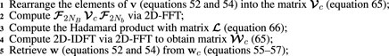
The key aspect of Algorithm 7 is replacing the matrix-vector products of CGLS (Algorithm 1) by fast convolutions (Algorithm 8). A fast convolution requires one 2D-DFT, one 2D-IDFT and an entrywise product of matrices. We consider that the 2D-DFT/IDFT are computed with 2D-FFT and requires λ (4D) log₂(4D) flops, where λ = 5 is compatible with a radix-2 FFT (Van Loan, 1992, p. 16), and the entrywise product 24D flops because it involves two complex matrices having 4D elements (Golub and Van Loan, 2013, p. 36). Hence, Algorithm 8 requires λ (16D) log₂(4D) + 26D flops, whereas a conventional matrix-vector multiplication involving a D × D matrix requires 2D² (Table 1). Finally, Algorithm 7 requires two 2D-FFTs (lines 4 and 5), one fast convolution and an inner product (line 8) previously to the while loop. Per iteration, there are three saxpys (lines 12, 15 and 16), two inner products (lines 14 and 17) and two fast convolutions (lines 13 and 17), so that:

$f_{\mathtt{T}\mathtt{O}\mathtt{B}\mathtt{2}\mathtt{0}}=\lambda \left(16D\right){\log }_2\left(4D\right)+26D+\mathtt{I}\mathtt{T}\mathtt{M}\mathtt{A}\mathtt{X}\left[\lambda \left(16D\right){\log }_2\left(4D\right)+58D\right].(67)$

7.8 Direct deconvolution

The method proposed by Takahashi et al. (2020, 2022) can be reformulated to avoid the iterations of the conjugate gradient method. This alternative formulation consists in considering that v = p and w = d in Eq. 52, where p is the parameter vector (Eq. 3) and d the observed data vector. In this case, the equality “=” in Eq. 52 becomes an approximation “≈ ”. Then, Eq. 64 is manipulated to obtain

${\mathcal{V}}_c\approx {\mathcal{F}}_{2N_B}^{*}\left[\left({\mathcal{F}}_{2N_B}{\mathcal{W}}_c{\mathcal{F}}_{2N_b}\right)◦\breve{\mathcal{L}}\right]{\mathcal{F}}_{2N_b}^{*},(68)$

where

$\breve{\mathcal{L}}={\mathcal{L}}^{*}\oslash \left(\mathcal{L}◦{\mathcal{L}}^{*}+\zeta \mathbf{1}\right),(69)$

1 is a 4D × 4D matrix of ones, “⊘” denotes entrywise division and ζ is a positive scalar. Note that ζ = 0 leads to $\mathbf{1}\oslash \mathcal{L}$. In this case, the entrywise division may be problematic due to the elements of $\mathcal{L}$ having absolute value equal or close to zero. So, a small ζ is set to avoid this problem in Eq. 69. Next, we use $\breve{\mathcal{L}}$ to obtain a matrix ${\mathcal{V}}_c$ from Eq. 68. Finally, the elements of the estimated parameter vector $\tilde{\mathbf{p}}$ are retrieved from the first quadrant of ${\mathcal{V}}_c$. This procedure represents a direct deconvolution (e.g., Aster et al., 2019, p. 220) using a Wiener filter (e.g., Gonzalez and Woods, 2002, p. 263).

The required total number of flops associated with the direct deconvolution aggregates one 2D-FFT to compute matrix $\mathcal{L}$ (Eq. 66), one entrywise product $\mathcal{L}◦{\mathcal{L}}^{*}$ involving complex matrices and one entrywise division to compute $\breve{\mathcal{L}}$ (Eq. 69) and a fast convolution (Algorithm 8) to evaluate Eq. 68, which results in:

$f_{\mathtt{d}\mathtt{e}\mathtt{c}\mathtt{o}\mathtt{n}\mathtt{v}.}=\lambda \left(12D\right){\log }_2\left(4D\right)+72D.(70)$

Differently from the convolutional equivalent-layer method proposed by Takahashi et al. (2020, 2022), the alternative direct deconvolution presented here produces an estimated parameter vector $\tilde{\mathbf{p}}$ directly from the observed data d, in a single step, avoiding the conjugate gradient iterations. On the other hand, the alternative method presented here requires estimating a set of tentative parameter vectors $\tilde{\mathbf{p}}$ for different predefined ζ. Besides, there must be criterion to chose the best $\tilde{\mathbf{p}}$ from this tentative set. This can be made, for example, by using the well-known L-curve (Hansen, 1992). From a computational point of view, the number of CGLS iterations in the method proposed by Takahashi et al. (2020, 2022) is equivalent to the number of tentative estimated parameter vectors required to form the L-curve in the proposed direct deconvolution.

8 Numerical simulations

8.1 Flops count

Figure 1 shows the total number of flops for solving the overdetermined problem (Eq. 22) with different equivalent-layer methods (Eqs. 27, 28, 35, 37, 38, 43, 50, 67 and 70), by considering the particular case in which H = I_P (Eq. 9; Subsection 3.2), μ = 0 (Eq. 11), W_d = I_D (Eq. 12) and $\bar{\mathbf{p}}=\mathbf{0}$ (Eq. 14), where I_P and I_D are the identities of order P and D, respectively. The flops are computed for different number of potential-field data ranging from 10,000 to 1,000,000. Figure 1 shows that the moving data-window strategy by using Leão and Silva’s 1989 method and direct deconvolution are the fastest methods.

FIGURE 1

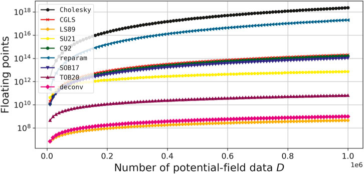
FIGURE 1. Total number of flops for different equivalent-layer methods (Eqs. 27, 28, 35, 37, 38, 43, 50, 67, and 70). The number of potential-field data D varies from 10,000 to 1,000,000.

The control parameters to run the equivalent-layer methods shown in Figure 1 are the following: 1) in CGLS, reparameterization approaches (e.g., Oliveira Jr. et al., 2013; Mendonça, 2020), Siqueira et al. (2017), and Takahashi et al. (2020) (Eqs. 28, 38, 43, 50, 67) we set $\mathtt{I}\mathtt{T}\mathtt{M}\mathtt{A}\mathtt{X}=50$; 2) Cordell (1992) we set ITMAX = 10 D; 3) in Leão and Silva (1989) (Eq. (35)) we set D′ = 49 (7 × 7) and P′ = 225 (15 × 15); and 4) in Soler and Uieda (2021) (Eq. (37)) we set D′ = P′ = 900 (30 × 30).

8.2 Synthetic potential-field data

We create a model composed of several rectangular prisms that can be split into three groups. The first is composed of 300 small cubes (not shown) with top at 0 m and side lengths defined according to a pseudo-random variable having uniform distribution from 100 to 200 m. Their density contrasts are defined by a pseudo-random variable uniformly distributed from 1,000 to 2000 kg/m³. These prisms produce the short-wavelength component of the simulated gravity data. The 4 prisms forming the second group of our model (indicated by A-D in Figure 2) have tops varying from 10 to 100 m and bottom from 1,010 to 1,500 m. They have density contrasts of 1,500, −1800, −3,000 and 1,200 kg/m³ and side lengths varying from 1,000 to 4,000 m. These prisms produce the mid-wavelength component of the simulated gravity data. There is also a single prism (indicated by E in Figure 2) with top at 1,000 m, bottom at 1,500 m and side lengths of 4,000 and 6,000 m. This prism has density contrast is −900 kg/m³ and produces the long-wavelength of our synthetic gravity data.

FIGURE 2

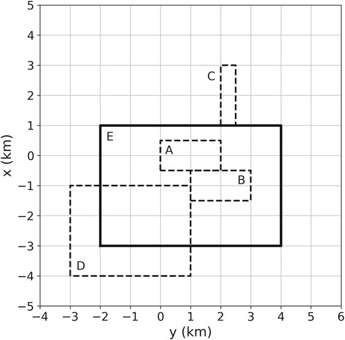
FIGURE 2. Synthetic prisms used in numerical simulations. The prisms A to D with horizontal projections represented by dashed lines have density contrasts of, respectively, 1,500, −1800, −3,000 and 1,200 kg/m³, tops varying from 10 to 100 m, bottom from 1,010 to 1,500 m and side lengths varying from 1,000 to 4,000 m. The prism E with horizontal projection represented by solid lines has a density contrast −900 kg/m³, top at 1,000 m, bottom at 1,500 m and side lengths of 4,000 and 6,000 m. Our model also have 300 additional small cubes (not shown), with top at 0 m and side lengths defined according to a pseudo-random variable having uniform distribution from 100 to 200 m. Their density contrasts vary randomly from 1,000 to 2000 kg/m³.

We have computed noise-free gravity disturbance and gravity-gradient tensor components produced by our model (Figure 2) on a regularly spaced grid of 50 × 50 points at z = −100 m (Figure 3). We have also simulated additional L = 20 gravity disturbance data sets d^ℓ, ℓ ∈ {1: L}, by adding pseudo-random Gaussian noise with zero mean and crescent standard deviations to the noise-free data (not shown). The standard deviations vary from 0.5% to 10% of the maximum absolute value in the noise-free data, which corresponds to 0.21 and 4.16 mGal, respectively.

FIGURE 3

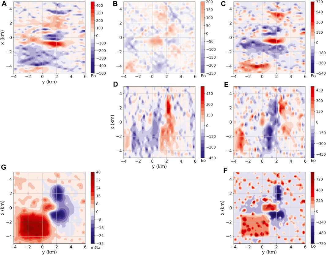
FIGURE 3. Noise-free gravity data produced by an ensemble of rectangular prisms (Figure 2). The data are located on a regular grid of 50×50 points. Panels (A–F) show, respectively, the xx, xy, xz, yy, yz and zz component of the gravity-gradient tensor in Eötvös (E). Panel (G) shows the gravity disturbance in milligals (mGal).

8.3 Stability analysis and gravity-gradient components

We set a planar equivalent layer of point masses having one source below each datum at a constant vertical coordinate z ≈ 512.24 m. This depth was set by following the Dampney’s (1969) criterion (see Subsection 2.1), so that the vertical distance Δz between equivalent sources and the simulated data is equal to 3× the grid spacing (Δx = Δy ≈ 204.08 m). Note that, in this case, the layer has a number of sources p equal to the number of data D.

We have applied the Cholesky factorization (Eqs. 25, 26), CGLS (Algorithm 1), column-action update method of Cordell (1992) (Algorithm 4), the iterative method of Siqueira et al. (2017) (Algorithm 6), the iterative deconvolution (Algorithm 7 and Algorithm 8) proposed by Takahashi et al. (2020) and the direct deconvolution (Eqs. 68 and 69) with four different values for the parameter ζ to the 21 gravity data sets.

For each method, we have obtained one estimate $\tilde{\mathbf{p}}$ from the noise-free gravity data d and L = 20 estimates ${\tilde{\mathbf{p}}}^{\ell }$ from the noise-corrupted gravity data d^ℓ, ℓ ∈ {1: L}, for the planar equivalent layer of point masses, totaling 21 estimated parameter vectors and 20 pairs $\left(\mathrm{\Delta }{p}^{\ell },\mathrm{\Delta }{d}^{\ell }\right)$ of model and data perturbations (Eqs. 30, 31). Figure 4 shows the numerical stability curves computed with each method for the synthetic gravity data.

FIGURE 4

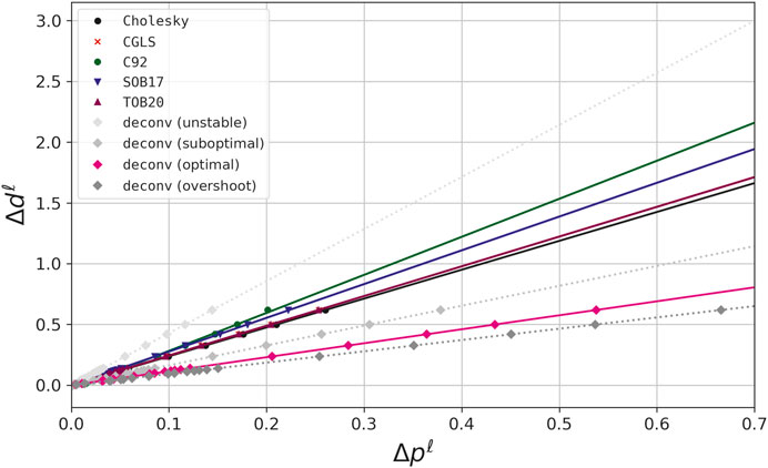
FIGURE 4. Numerical stability curves obtained for the 21 synthetic gravity data sets by using the Cholesky factorization with μ ≈2×10⁻²; column-action update $(\mathtt{C}\mathtt{9}\mathtt{2})$ with 25,000 iterations (10× the number D of potential-field data); CGLS, iterative method $(\mathtt{S}\mathtt{O}\mathtt{B}\mathtt{1}\mathtt{7})$ and iterative deconvolution $(\mathtt{T}\mathtt{O}\mathtt{B}\mathtt{2}\mathtt{0})$ with 50 iterations each (Algorithm 1, Algorithm 6 and Algorithm 7); and the direct deconvolution $(\mathtt{d}\mathtt{e}\mathtt{c}\mathtt{o}\mathtt{n}\mathtt{v}.)$ computed with four different values for ζ (Eq. 69): 0, 10^–18 (overshoot), 10^–22 (optimal) and 10^–28 (suboptimal). The stability parameter κ (Eq. 29) obtained for the eight curves described above are 2.37 $(\mathtt{C}\mathtt{h}\mathtt{o}\mathtt{l}\mathtt{e}\mathtt{s}\mathtt{k}\mathtt{y})$; 2.45 $(\mathtt{C}\mathtt{G}\mathtt{L}\mathtt{S})$; 3.13 $(\mathtt{C}\mathtt{9}\mathtt{2})$; 2.78 $(\mathtt{S}\mathtt{O}\mathtt{B}\mathtt{1}\mathtt{7})$; 2.44 $(\mathtt{T}\mathtt{O}\mathtt{B}\mathtt{2}\mathtt{0})$; 4.28, 1.63, 1.15 and 0.93 ($\mathtt{d}\mathtt{e}\mathtt{c}\mathtt{o}\mathtt{n}\mathtt{v}.$ with null, suboptimal, optimal and overshoot ζ).

All these 21 estimated parameters vectors were obtained by solving the overdetermined problem (Eq. 22) with the same method for the particular case in which H = I (Eq. 9; Subsection 3.2), W_d = W_q = I (Eqs. 12, 13) and $\bar{\mathbf{p}}=\mathbf{0}$ (Eq. 14), where I is the identity of order D.

Figure 4 shows how the numerical stability curves vary as the level of the noise is increased. We can see that for all methods, a linear tendency is observed as it is expected. The inclination of the straight line indicates the stability of each method. As shown in Figure 4, the direct deconvolution with ζ = 0 exhibits a high slope, which indicates high instability and emphasizes the necessity of using the Wiener filter (ζ > 0 in Eq. 69).

The estimated stability parameters κ (Eq. 29) obtained for the Cholesky factorization, CGLS and iterative deconvolution are close to each other (Figure 4). They are slightly smaller than that obtained for the iterative method of Siqueira et al. (2017). Note that by varying the parameter ζ (Eq. 69) it is possible to obtain different stability parameters κ for the direct deconvolution. There is no apparent rule to set ζ. A practical criterion can be the maximum ζ producing a satisfactory data fit. Overshoot values tend to exaggeratedly smooth the predicted data. As we can see in Figure 4, the most unstable approaches are the direct deconvolution with null ζ $(\mathtt{d}\mathtt{e}\mathtt{c}\mathtt{o}\mathtt{n}\mathtt{v}.\mathtt{u}\mathtt{n}\mathtt{s}\mathtt{t}\mathtt{a}\mathtt{b}\mathtt{l}\mathtt{e})$, followed by the column-action update $(\mathtt{C}\mathtt{9}\mathtt{2})$.

We inverted the noise-corrupted gravity disturbance with the highest noise level (not shown) to estimate an equivalent layer (not shown) via iterative deconvolution (Algorithm 7). Figure 5G shows the residuals (in mGal) between the predicted and noise-corrupted gravity disturbances. As we can see, the residuals are uniformly distributed on simulated area and suggest that the equivalent layer produces a good data fit. This can be verified by inspecting the histogram of the residuals between the predicted and noise-corrupted gravity disturbances shown in panel (G) of Figure 6.

FIGURE 5

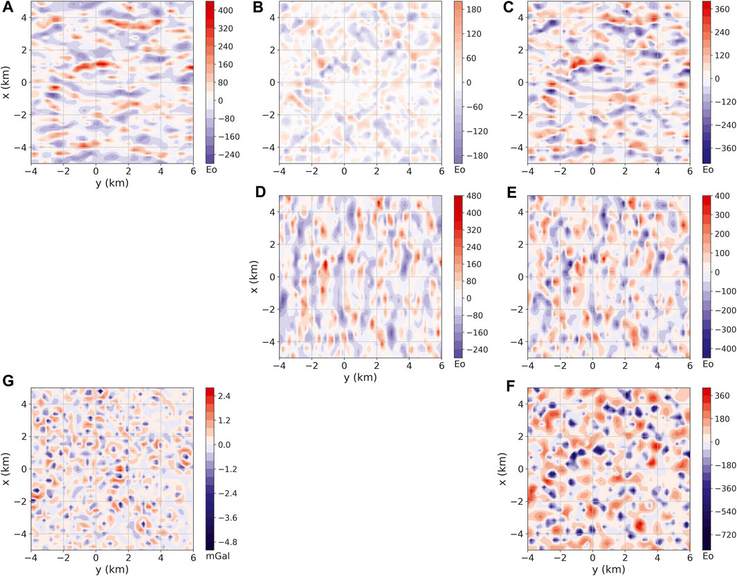
FIGURE 5. Residuals between the gravity data predicted by the equivalent layer estimated with the iterative deconvolution $(\mathtt{T}\mathtt{O}\mathtt{B}\mathtt{2}\mathtt{0})$ (Algorithm 7). The inverse problems was solved by using the noise-corrupted gravity disturbance having the maximum noise level (not shown). Panels (A–F) show the residuals between the predicted and noise-free gravity gradient data (Figure 3) associated with the xx, xy, xz, yy, yz and zz components of the gravity-gradient tensor, respectively. The values are in Eötvös. (G) Shows the residuals between the predicted and noise-corrupted gravity disturbances. The values are in milligals (mGal).

FIGURE 6

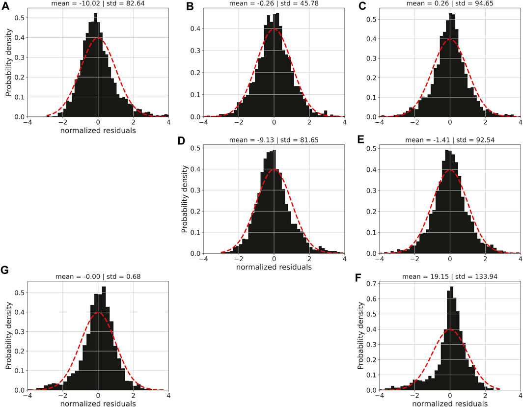
FIGURE 6. Histograms of the residuals shown in Figure 5. The residuals were normalized by removing the mean and dividing the difference by the standard deviation. Panels (A–F) show the histograms associated with the xx, xy, xz, yy, yz and zz components of the gravity-gradient tensor, respectively. (G) Shows the histogram of the residuals between the predicted and noise-corrupted gravity disturbances.

Using the estimated layer, we have computed the gravity-gradient data (not shown) at the observations points. Figure 5A–F show the residuals (in Eötvös) between the predicted (not shown) and noise-free gravity-gradient data (Figure 3). These figures show that the iterative deconvolution (Algorithm 7) could predict the six components of the gravity-gradient tensor with a good precision, which can also be verified in the corresponding histograms shown in Figure 6.

In the Supplementary Material, we show the residuals between the gravity data predicted by the equivalent layer estimated by using the following methods: 1) the CGLS method (Algorithm 1); 2) the Cholesky factorization (Eqs. 25, 26); 3) the iterative method proposed by Siqueira et al. (2017) (Algorithm 6); 4) the direct deconvolution with optimal value of ζ = 10^–22 (Eq. 69); and 5) the iterative method proposed by Cordell (1992) (Algorithm 4).

9 Applications to field data

In this section, we show the results obtained by applying the iterative deconvolution (Algorithm 7) to a field data set over the Carajás Mineral Province (CMP) in the Amazon craton (Moroni et al., 2001; Villas and Santos, 2001). This area (Figure 7) is known for its intensive mineral exploration such as iron, copper, gold, manganese, and, recently, bauxite.

FIGURE 7

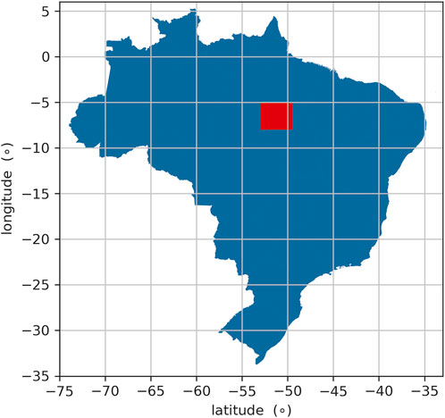
FIGURE 7. Location of the Carajás Mineral Province (CMP), Brazil. The coordinates are referred to the WGS-84 datum. The study area (shown in red) is located at the UTM zone 22S.

9.1 Geological setting

The Amazon Craton is one of the largest and least-known Archean-Proterozoic areas in the world, comprehending a region with a thousand square kilometers. It is one of the main tectonic units in South America, which is covered by five Phanerozoic basins: Maranhão (Northeast), Amazon (Central), Xingu-Alto Tapajós (South), Parecis (Southwest), and Solimões (West). The Craton is limited by the Andean Orogenic Belt to the west and the by Araguaia Fold Belt to the east and southeast. The Amazon craton has been subdivided into provinces according to two models, one geochronological and the other geophysical-structural (Amaral, 1974; Teixeira et al., 1989; Tassinari and Macambira, 1999). Thus, seven geological provinces with distinctive ages, evolution, and structural patterns can be observed, namely,: 1) Carajás with two domains - the Mesoarchean Rio Maria and Neoarchean Carajás; 2) Archean-Paleoproterozoic Central Amazon, with Iriri-Xingu and Curuá-Mapuera domains; 3) Trans-Amazonian (Ryacian), with the Amapá and Bacajá domains; 4) the Orosinian Tapajós-Parima, with Peixoto de Azevedo, Tapajós, Uaimiri, and Parima domains; 5) Rondônia-Juruena (Statherian), with Jamari, Juruena, and Jauru domains; 6) The Statherian Rio Negro, with Rio Negro and Imeri domains; and 7) Sunsás (Meso-Neoproterozoic), with Santa Helena and Nova Brasilândia domains (Santos et al., 2000). Nevertheless, we focus this work only on the Carajás Province.

The Carajás Mineral Province (CMP) is located in the east-southeast region of the craton (Figure 7), within an old tectonically stable nucleus in the South American Plate that became tectonically stable at the beginning of Neoproterozoic (Salomao et al., 2019). This area has been the target of intensive exploration at least since the final of the ’60s, after the discovery of large iron ore deposits. There are several greenstone belts in the region, among them are the Andorinhas, Inajá, Cumaru, Carajás, Serra Leste, Serra Pelada, and Sapucaia (Santos et al., 2000). The mineralogic and petrologic studies in granite stocks show a variety of minerals found in the province, such as amphibole, plagioclase, biotite, ilmenite, and magnetite (Cunha et al., 2016).

9.2 Potential-field data

The field data used here were obtained from an airborne survey conducted by Lasa Prospecções S/A. and Microsurvey Aerogeofísica Consultoria Científica Ltda. between April/2013 and October/2014. The survey area covers $\approx 58000{\mathrm{k}\mathrm{m}}^2$ between latitudes −8°/− 5° and longitudes −53°/− 49.5° referred to the WGS-84 datum. We obtained the horizontal coordinates x and y already in the UTM zone 22S. The flight and tie lines are spaced at 3 km and 12 km, with orientation along directions N − S and E − W, respectively. The data are placed at an approximately constant distance of 900 m above the ground. Figure 8 shows the D = 500, 000 aerogravimetric data on a grid of 1,000 × 500 observation points with Δx = 358.12 m and Δy = 787.62 m.

FIGURE 8

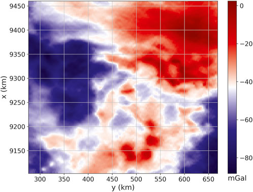
FIGURE 8. Field aerogravimetric data over Carajás, Brazil. There are D =500,000 observations located on regular grid of 1,000×500 points.

9.3 Potential-field transformation

We applied the equivalent-layer technique to the observed data (Figure 8) with the purpose of illustrating how to estimate the gravity-gradient tensor over the study area. We used an equivalent layer layout with one source located below each datum (so that P = D) on a horizontal plane having a vertical distance Δz ≈ 2362.86 m from the observation plane. This setup is defined by setting Δz ≈ 3 dy, which follows the same strategy of Reis et al. (2020). We solve the linear inverse problem for estimating the physical-property distribution on the layer by using the iterative deconvolution (Algorithm 7) with a maximum number of 50 iterations. Actually, the algorithm have converged with only 18 iterations.

Figure 9G shows the histogram of the residuals between the predicted (not shown) and observed data (Figure 8). As we can see, the iterative deconvolution produced an excellent data fit. By using the estimated layer, we have computed the gravity-gradient tensor components at the observation points. The results are shown in Figure 9A–F.

FIGURE 9

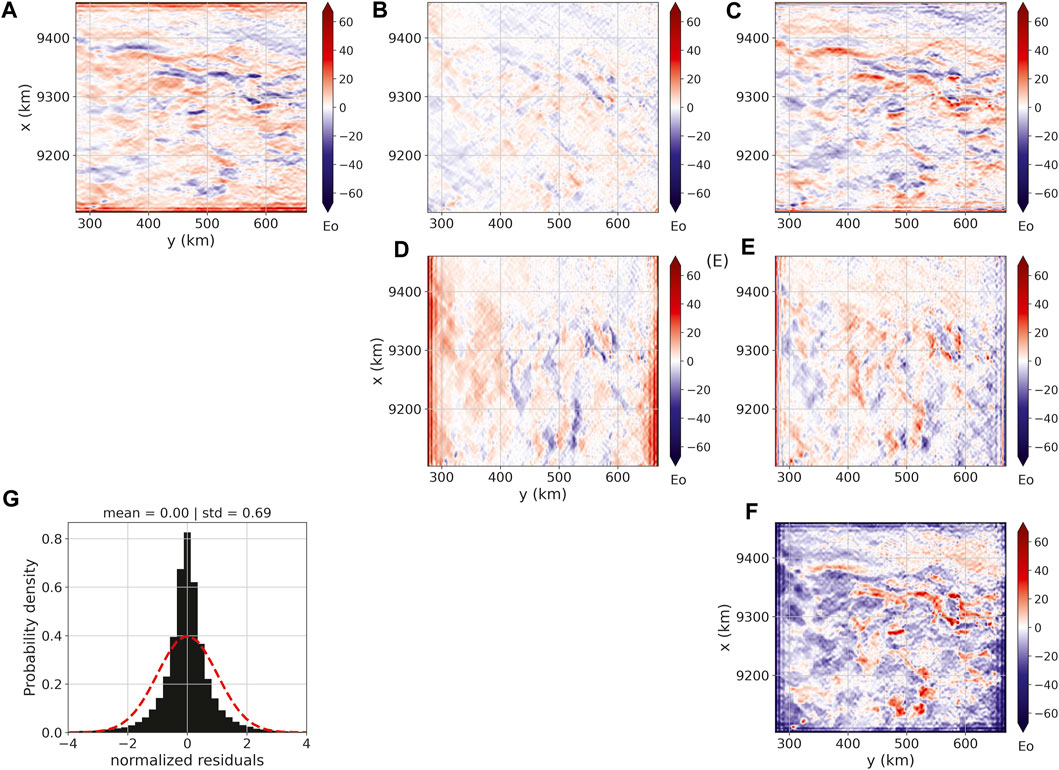
FIGURE 9. Estimated gravity-gradient tensor components over Carajás, Brazil. Panels (A–F) show, respectively, the xx, xy, xz, yy, yz and zz components of the gravity-gradient tensor in Eötvös. Panel (G) shows the histogram of the residuals between predicted data (not shown) and field data (Figure 8). The residuals were normalized by removing the mean and dividing the difference by the standard deviation. The results were generated by applying the iterative deconvolution $(\mathtt{T}\mathtt{O}\mathtt{B}\mathtt{2}\mathtt{0})$ (Algorithm 7) with 50 iterations.

Considering the processing time, the iterative deconvolution took $\approx 1.98\mathrm{s}$ to execute the 18 iterations for estimating the physical-property distribution on the layer by inverting the D = 500, 000 observed data. The code was run in a modest computer with 16, 0 GiB of memory and processor 12th Gen Intel^® Core™ i9 − 12900H × 20. Given the estimated equivalent layer, the gravity-gradient components shown in Figure 9 were computed in $\approx 3.41\mathrm{s}$. These results demonstrate the efficiency of the iterative deconvolution method in processing large datasets.

10 Discussion

The review discusses strategies utilized to reduce the computational cost of the equivalent-layer technique for processing potential-field data. These strategies are often combined in developed methods to efficiently handle large-scale data sets. Next, the computational strategies are addressed. All results shown here were generated with the Python package gravmag (https://doi.org/10.5281/zenodo.8284769). The datasets generated for this study can be found in the online repository: https://github.com/pinga-lab/eqlayer-review-computational.

The first one is the moving data-window scheme spanning the data set. This strategy solves several much smaller, regularized linear inverse problems instead of a single large one. Each linear inversion is solved using the potential-field observations and equivalent sources within a given moving window and can be applied to both regularly or irregularly spaced data sets. If the data and the sources are distributed on planar and regularly spaced grids, this strategy offers a significant advantage because the sensitivity submatrix of a given moving window remains the same for all windows. Otherwise, the computational efficiency of the equivalent-layer technique using the moving-window strategy decreases because the sensitivity submatrix for each window must be computed.

The second and third strategies, referred to as the column-action and row-action updates, involve iteratively calculating a single column and a single row of the sensitivity matrix, respectively. By following the column-action update strategy, a single column of the sensitivity matrix is calculated during each iteration. This implies that a single equivalent source contributes to the fitting of data in each iteration. Conversely, in the row-action update strategy, a single row of the sensitivity matrix is calculated per iteration, which means that one potential-field observation is incorporated in each iteration, forming a new subset of equivalent data much smaller than the original data. Both strategies (column- and row-action updates) have a great advantage because a single column or a single row of the sensitivity matrix is calculated iteratively. However, to our knowledge, the strategy of the column-action update presents some issues related to convergence, and the strategy of the row-action update can also have issues if the number of equivalent data is not significantly smaller than the original number of data points.

The fourth strategy is the sparsity induction of the sensitivity matrix using wavelet compression, which involves transforming a full sensitivity matrix into a sparse one with only a few nonzero elements. The developed equivalent-layer methods using this strategy achieve sparsity by setting matrix elements to zero if their values are smaller than a predefined threshold. We highlight two methods that employ the sparsity induction strategy. The first method, known as wavelet-compression equivalent layer, compresses the coefficients of the original sensitivity matrix using discrete wavelet transform, achieves sparsity in the sensitivity matrix, and solves the inverse problem in the wavelet domain without an explicit regularization parameter. The regularized solution in the wavelet domain is estimated using a conjugate gradient (CG) least squares algorithm, where the number of iterations serves as a regularization factor. The second equivalent-layer method that uses the sparsity induction strategy applies quadtree discretization of the parameters over the equivalent layer, achieves sparsity in the sensitivity matrix, and solves the inverse problem using CG algorithm. In quadtree discretization, equivalent sources located far from the observation point are grouped together to form larger equivalent sources, reducing the number of parameters to be estimated. Computationally, the significant advantage of the equivalent-layer methods employing wavelet compression and quadtree discretization is the sparsity induction in the sensitivity matrix, which allows for fast iteration of the CG algorithm. However, we acknowledge that this strategy requires computing the full and dense sensitivity matrix, which can be considered a drawback when processing large-scale potential-field data.

The fifth strategy is the reparametrization of the original parameters to be estimated in the equivalent-layer technique. In this strategy, the developed equivalent-layer methods reduce the dimension of the linear system of equations to be solved by estimating a lower-dimensional parameter vector. We highlight two methods that used the reparametrization strategy: 1) the polynomial equivalent layer (PEL) and; 2) the lower-dimensional subspace of the equivalent layer. In the PEL, there is an explicit reparametrization of the equivalent layer by representing the unknown distribution over the equivalent layer as a set of piecewise-polynomial functions defined on a set of equivalent-source windows. The PEL method estimates the polynomial coefficients of all equivalent-source windows. Hence, PEL reduces the dimension of the linear system of equations to be solved because the polynomial coefficients within all equivalent-source windows are much smaller than both the number of equivalent sources and the number of data points. In the lower-dimensional subspace of the equivalent layer, there is an implicity reparametrization of the equivalent layer by reducing the linear system dimension from the original and large-model space to a lower-dimensional subspace. The lower-dimensional subspace is grounded on eigenvectors of the matrix composed by the gridded data set. The main advantage of the reparametrization of the equivalent layer is to deal with lower-dimensional linear system of equations. However, we acknowledge that this strategy may impose an undesirable smoothing effect on both the estimated parameters over the equivalent layer and the predicted data.

The sixth strategy involves an iterative scheme in which the estimated distribution over the equivalent layer is updated iteratively. Following this strategy, the developed equivalent-layer methods differ either in terms of the expression used for the estimated parameter correction or the domain utilized (wavenumber or space domains). The iterative estimated correction may have a physical meaning, such as the excess mass constraint. All the iterative methods are efficient as they can handle irregularly spaced data on an undulating surface, and the updated corrections for the parameter vector at each iteration are straightforward, involving the addition of a quantity proportional to the data residual. However, they have a disadvantage because the iterative strategy requires computing the full and dense sensitivity matrix to compute the predicted and residual data in all observation stations per iteration.

The seventh strategy is called iterative deconvolutional of the equivalent layer. This strategy deals with regularly spaced grids of data stations and equivalent sources which are located at a constant height and depth, respectively. Specifically, one source is placed directly below each observation station, which results in sensitivity matrices with a BTTB (Block-Toeplitz Toeplitz-Block) structure. It is possible to embed the BTTB matrix into a matrix of Block-Circulant Circulant-Block (BCCB) structure, which requires only one equivalent source. This allows for fast matrix-vector product using a 2D fast Fourier transform (2D FFT). As a result, the potential-field forward modeling can be calculated using a 2D FFT with only one equivalent source required. The main advantages of this strategy are that the entire sensitivity matrices do not need to be formed or stored; only their first columns are required. Additionally, it allows for a highly efficient iteration of the CG algorithm. However, the iterative deconvolutional of the equivalent layer requires observations and equivalent sources aligned on a horizontal and regularly-spaced grid.

The eigth strategy is a direct deconvolution method, which is a mathematical process very common in geophysics. However, to our knowledge, direct deconvolution has never been used to solve the inverse problem associated with the equivalent-layer technique. From the mathematical expressions in the iterative deconvolutional equivalent layer with BTTB matrices, direct deconvolution arises naturally since it is an operation inverse to convolution. The main advantage of applying the direct deconvolution strategy in the equivalent layer is that it avoids, for example, the iterations of the CG algorithm. However, the direct deconvolution is known to be an unstable operation. To mitigate this instability, the Wiener deconvolution method can be adopted.

Table 2 presents a list of computational strategies used in the equivalent-layer technique to reduce the computational demand. The table aims to emphasize the important characteristics, advantages, and disadvantages of each computational strategy. Additionally, it highlights the available methods that use each strategy.

TABLE 2

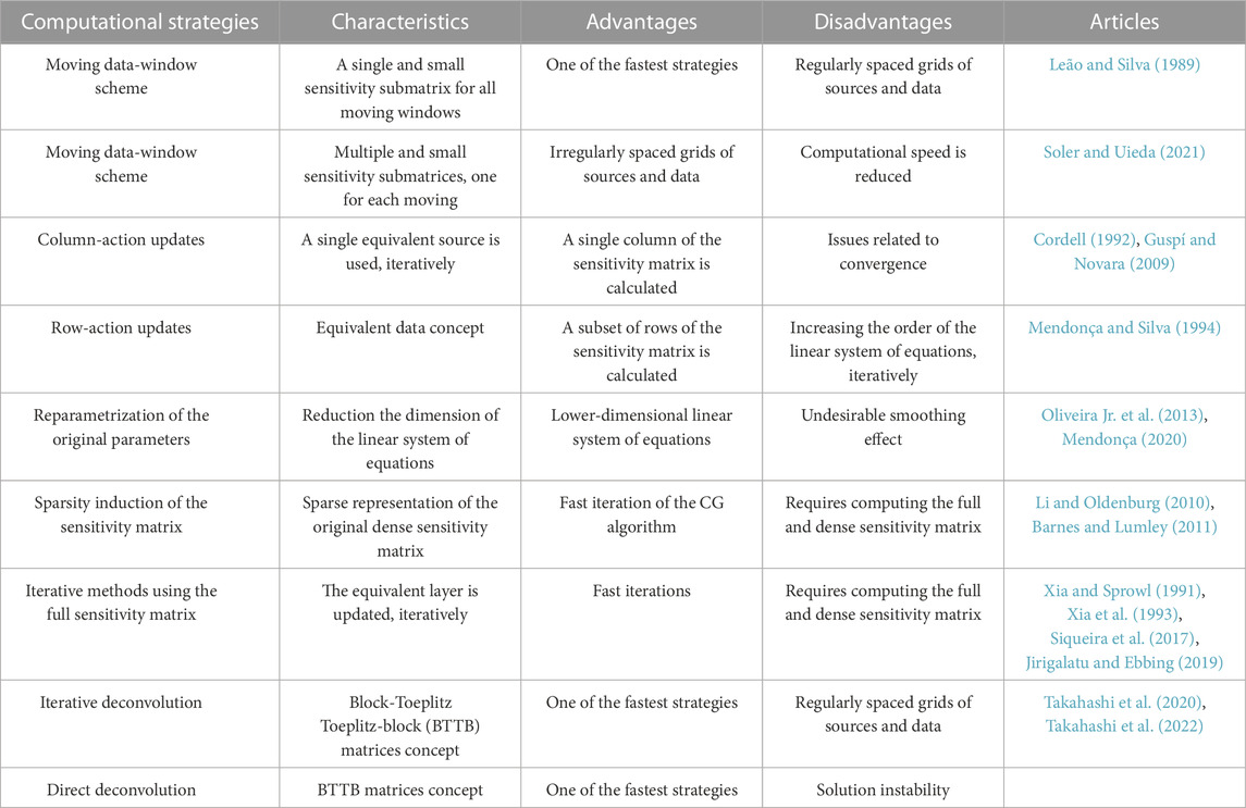
TABLE 2. Computational strategies to overcome the intensive computational cost of the equivalent-layer technique for processing potential-field data and the corresponding articles.

11 Conclusion

We have presented a comprehensive review of the strategies used to tackle the intensive computational cost associated with processing potential-field data using the equivalent-layer technique. Each of these strategies is rarely used individually; rather, some developed equivalent-layer methods combine more than one strategy to achieve computational efficiency when dealing with large-scale data sets. We focuses on the following specific strategies: 1) the moving data-window scheme; 2) the column-action and row-action updates; 3) the sparsity induction of the sensitivity matrix; 4) the reparametrization of the original parameters; 5) the iterative scheme using the full sensitivity matrix; 6) the iterative deconvolution; and 7) the direct deconvolution. Taking into account the mathematical bases used in the above-mentioned strategies, we have identified five groups: 1) the reduction of the dimensionality of the linear system of equations to be solved; 2) the generation of a sparse linear system of equations to be solved; 3) the explicit iterative method; 4) the improvement in forward modeling; and 5) the deconvolution using the concept of block-Toeplitz Toeplitz-block (BTTB) matrices.

We show in this review that the computational cost of the equivalent layer can vary from up to 10⁹ flops depending on the method without compromising the linear system stability. The moving data-window scheme and direct deconvolution are the fastest methods; however, they both have drawbacks. To be computationally efficient, the moving data-window scheme and the direct deconvolution require data and equivalent sources that are distributed on planar and regularly spaced grids. Moreover, they both requires choosing an optimun parameter of stabilization. We stress that the direct deconvolution has an aditional disadvantage in terms of a higher data residual and border effects over the equivalent layer after processing. These effects can be seen from the upward continuation of the real data from Carajás.

We draw the readers’ attention to the possibility of combining more than one aforementioned strategies for reducing the computational cost of the equivalent-layer technique.

Author contributions

VO and VB: Study conception and mathematical deductions. VO: Algorithms. VO and DT: Python codes and synthetic data applications. VO and AR: Real data applications. VO and VB: Result analysis and draft manuscript preparation.

Funding

VB was supported by fellowships from CNPq (grant 309624/2021-5) and FAPERJ (grant 26/202.582/2019). VO was supported by fellowships from CNPq (grant 315768/2020-7) and FAPERJ (grant E-26/202.729/2018). DT was supported by a Post-doctoral scholarship from CNPq (grant 300809/2022-0).

Acknowledgments

We thank the brazillian federal agencies CAPES, CNPq, state agency FAPERJ and Observatório Nacional research institute and Universidade do Estado do Rio de Janeiro.

Conflict of interest

The authors declare that the research was conducted in the absence of any commercial or financial relationships that could be construed as a potential conflict of interest.

Publisher’s note

All claims expressed in this article are solely those of the authors and do not necessarily represent those of their affiliated organizations, or those of the publisher, the editors and the reviewers. Any product that may be evaluated in this article, or claim that may be made by its manufacturer, is not guaranteed or endorsed by the publisher.

Supplementary material

The Supplementary Material for this article can be found online at: https://www.frontiersin.org/articles/10.3389/feart.2023.1253148/full#supplementary-material

References

Amaral, G. (1974). Geologia Pré-Cambriana da Região Amazônica. Ph.D. thesis, Universidade de ãão Paulo.

Google Scholar

Aster, R. C., Borchers, B., and Thurber, C. H. (2019). Parameter estimation and inverse problems. 3 edn. Elsevier.

Google Scholar

Barbosa, V. C. F., Silva, J. B., and Medeiros, W. E. (1997). Gravity inversion of basement relief using approximate equality constraints on depths. Geophysics 62, 1745–1757. doi:10.1190/1.1444275

CrossRef Full Text | Google Scholar

Barnes, G., and Lumley, J. (2011). Processing gravity gradient data. GEOPHYSICS 76, I33–I47. doi:10.1190/1.3548548

CrossRef Full Text | Google Scholar

Blakely, R. J. (1996). Potential theory in gravity and magnetic applications. Cambridge University press.

Google Scholar

Bott, M. H. P. (1960). The use of rapid digital computing methods for direct gravity interpretation of sedimentary basins. Geophys. J. Int. 3, 63–67. doi:10.1111/j.1365-246X.1960.tb00065.x

CrossRef Full Text | Google Scholar

Chan, R. H.-F., and Jin, X.-Q. (2007). An introduction to iterative Toeplitz solvers, 5. SIAM.

Google Scholar

Cordell, L. (1992). A scattered equivalent-source method for interpolation and gridding of potential-field data in three dimensions. Geophysics 57, 629–636. doi:10.1190/1.1443275

CrossRef Full Text | Google Scholar

Cunha, I. R., Dall’Agnol, R., and Feio, G. R. L. (2016). Mineral chemistry and magnetic petrology of the archean Planalto Suite, Carajás Province – amazonian Craton: implications for the evolution of ferroan archean granites. J. S. Am. Earth Sci. 67, 100–121. doi:10.1016/j.jsames.2016.01.007

CrossRef Full Text | Google Scholar

Dampney, C. N. G. (1969). The equivalent source technique. GEOPHYSICS 34, 39–53. doi:10.1190/1.1439996

CrossRef Full Text | Google Scholar

Davis, P. J. (1979). Circulant matrices. John Wiley & Sons, Inc.

Google Scholar

Elfving, T., Hansen, P. C., and Nikazad, T. (2017). Convergence analysis for column-action methods in image reconstruction. Numer. Algorithms 74, 905–924. doi:10.1007/s11075-016-0176-x

CrossRef Full Text | Google Scholar

Emilia, D. A. (1973). Equivalent sources used as an analytic base for processing total magnetic field profiles. GEOPHYSICS 38, 339–348. doi:10.1190/1.1440344

CrossRef Full Text | Google Scholar

Golub, G. H., and Van Loan, C. F. (2013). Johns hopkins studies in the mathematical sciences. 4 edn. Johns Hopkins University Press.Matrix computations.

Google Scholar

Gonzalez, R. C., and Woods, R. E. (2002). Digital image processing. 2 edn. Prentice Hall.

Google Scholar

Gonzalez, S. P., Barbosa, V. C. F., and Oliveira, V. C. (2022). Analyzing the ambiguity of the remanent-magnetization direction separated into induced and remanent magnetic sources. J. Geophys. Res. Solid Earth 127, 1–24. doi:10.1029/2022JB024151

CrossRef Full Text | Google Scholar

Guspí, F., Introcaso, A., and Introcaso, B. (2004). Gravity-enhanced representation of measured geoid undulations using equivalent sources. Geophys. J. Int. 159, 1–8. doi:10.1111/j.1365-246X.2004.02364.x

CrossRef Full Text | Google Scholar

Guspí, F., and Novara, I. (2009). Reduction to the pole and transformations of scattered magnetic data using Newtonian equivalent sources. GEOPHYSICS 74, L67–L73. doi:10.1190/1.3170690

CrossRef Full Text | Google Scholar

Hansen, P. C. (1992). Analysis of discrete ill-posed problems by means of the l-curve. SIAM Rev. 34, 561–580. doi:10.1137/1034115

CrossRef Full Text | Google Scholar

Hansen, R. O., and Miyazaki, Y. (1984). Continuation of potential fields between arbitrary surfaces. GEOPHYSICS 49, 787–795. doi:10.1190/1.1441707

CrossRef Full Text | Google Scholar

Horn, R. A., and Johnson, C. R. (1991). Topics in matrix analysis. 1 edn. Cambridge University Press.

Google Scholar

Jain, A. K. (1989). Fundamentals of digital image processing. 1 edn. Pearson.

Google Scholar

Jirigalatu, , and Ebbing, J. (2019). A fast equivalent source method for airborne gravity gradient data. Geophysics 84, G75–G82. doi:10.1190/GEO2018-0366.1

CrossRef Full Text | Google Scholar

Kellogg, O. D. (1967). Foundations of potential theory. Springer-Verlag. reprint from the first edition of 1929 edn.

Google Scholar

Kennett, B., Sambridge, M., and Williamson, P. (1988). Subspace methods for large inverse problems with multiple parameter classes. Geophys. J. Int. 94, 237–247. doi:10.1111/j.1365-246X.1988.tb05898.x

CrossRef Full Text | Google Scholar

Leão, J. W. D., and Silva, J. B. C. (1989). Discrete linear transformations of potential field data. Geophysics 54, 497–507. doi:10.1190/1.1442676

CrossRef Full Text | Google Scholar

Li, Y., Nabighian, M., and Oldenburg, D. W. (2014). Using an equivalent source with positivity for low-latitude reduction to the pole without striation. GEOPHYSICS 79, J81–J90. doi:10.1190/geo2014-0134.1

CrossRef Full Text | Google Scholar

Li, Y., and Oldenburg, D. W. (2010). Rapid construction of equivalent sources using wavelets. GEOPHYSICS 75, L51–L59. doi:10.1190/1.3378764

CrossRef Full Text | Google Scholar

Mendonça, C. A., and Silva, J. B. C. (1994). The equivalent data concept applied to the interpolation of potential field data. Geophysics 59, 722–732. doi:10.1190/1.1443630

CrossRef Full Text | Google Scholar

Mendonça, C. A. (2020). Subspace method for solving large-scale equivalent layer and density mapping problems. GEOPHYSICS 85, G57–G68. doi:10.1190/geo2019-0302.1

CrossRef Full Text | Google Scholar

Menke, W. (2018). Geophysical data analysis: Discrete inverse theory. 4 edn. Elsevier.

Google Scholar

Moroni, M., Girardi, V., and Ferrario, A. (2001). The Serra Pelada Au-pge deposit, Serra dos Carajás (pará state, Brazil): geological and geochemical indications for a composite mineralising process. Miner. Deposita 36, 768–785. doi:10.1007/s001260100201

CrossRef Full Text | Google Scholar

Oldenburg, D., McGillivray, P., and Ellis, R. (1993). Generalized subspace methods for large-scale inverse problems. Geophys. J. Int. 114, 12–20. doi:10.1111/j.1365-246X.1993.tb01462.x

CrossRef Full Text | Google Scholar

Oliveira, V. C., Barbosa, V. C. F., and Uieda, L. (2013). Polynomial equivalent layer. GEOPHYSICS 78, G1–G13. doi:10.1190/geo2012-0196.1

CrossRef Full Text | Google Scholar

Press, W. H., Teukolsky, S. A., Vetterling, W. T., and Flannery, B. P. (2007). Numerical recipes: The art of scientific computing. 3 edn. Cambridge University Press.

Google Scholar

Reis, A. L. A., Oliveira, V. C., and Barbosa, V. C. F. (2020). Generalized positivity constraint on magnetic equivalent layers. Geophysics 85, 1–45. doi:10.1190/geo2019-0706.1

CrossRef Full Text | Google Scholar

Roy, A. (1962). Ambiguity in geophysical interpretation. GEOPHYSICS 27, 90–99. doi:10.1190/1.1438985

CrossRef Full Text | Google Scholar

Salomao, G. N., Dall’Agnol, R., Angelica, R. S., Figueiredo, M. A., Sahoo, P. K., Medeiros-Filho, C. A., et al. (2019). Geochemical mapping and estimation of background concentrations in soils of Carajás mineral province, eastern Amazonian Craton, Brazil. Geochem. Explor. Environ. Anal. 19, 431–447. doi:10.1144/geochem2018-066

CrossRef Full Text | Google Scholar

Santos, J. O. S., Hartmann, L. A., Gaudette, H. E., Groves, D. I., Mcnaughton, M. J., and Fletcher, I. R. (2000). A new understanding of the provinces of the Amazon Craton based on integration of field mapping and U-Pb and Sm-Nd geochronology. Gondwana Res. 3, 453–488. doi:10.1016/S1342-937X(05)70755-3

CrossRef Full Text | Google Scholar

Silva, J. B. C. (1986). Reduction to the pole as an inverse problem and its application to low-latitude anomalies. GEOPHYSICS 51, 369–382. doi:10.1190/1.1442096

CrossRef Full Text | Google Scholar

Siqueira, F., Oliveira, V. C., and Barbosa, V. C. F. (2017). Fast iterative equivalent-layer technique for gravity data processing: A method grounded on excess mass constraint. GEOPHYSICS 82, G57–G69. doi:10.1190/GEO2016-0332.1

CrossRef Full Text | Google Scholar

Skilling, J., and Bryan, R. (1984). Maximum entropy image reconstruction-general algorithm. Mon. Notices R. Astronomical Soc. 211(1), 111. doi:10.1093/mnras/211.1.111

CrossRef Full Text | Google Scholar

Soler, S. R., and Uieda, L. (2021). Gradient-boosted equivalent sources. Geophys. J. Int. 227, 1768–1783. doi:10.1093/gji/ggab297

CrossRef Full Text | Google Scholar

Takahashi, D., Oliveira, V. C., and Barbosa, V. C. (2022). Convolutional equivalent layer for magnetic data processing. Geophysics 87, 1–59. doi:10.1190/geo2021-0599.1

CrossRef Full Text | Google Scholar

Takahashi, D., Oliveira, V. C., and Barbosa, V. C. F. (2020). Convolutional equivalent layer for gravity data processing. GEOPHYSICS 85, G129–G141. doi:10.1190/geo2019-0826.1

CrossRef Full Text | Google Scholar

Tassinari, C. C., and Macambira, M. J. (1999). Geochronological provinces of the amazonian craton. Episodes 22, 174–182. doi:10.18814/epiiugs/1999/v22i3/004

CrossRef Full Text | Google Scholar

Teixeira, W., Tassinari, C., Cordani, U. G., and Kawashita, K. (1989). A review of the geochronology of the Amazonian Craton: tectonic implications. Precambrian Res. 42, 213–227. doi:10.1016/0301-9268(89)90012-0

CrossRef Full Text | Google Scholar

van der Sluis, A., and van der Vorst, H. A. (1987). “Numerical solution of large, sparse linear algebraic systems arising from tomographic problems,” in Seismic tomography with applications in global seismology and exploration geophysics. Editor G. Nolet (D. Reidel Publishing Company). chap. 3. 49–83.

CrossRef Full Text | Google Scholar

Van Loan, C. F. (1992). Computational frameworks for the fast fourier transform. Front. Appl. Math. (SIAM). doi:10.1137/1.9781611970999

CrossRef Full Text | Google Scholar

Villas, R. N., and Santos, M. (2001). Gold deposits of the Carajás mineral province: deposit types and metallogenesis. Miner. Deposita 36, 300–331. doi:10.1007/s001260100178

CrossRef Full Text | Google Scholar

Xia, J., Sprowl, D. R., and Adkins-Heljeson, D. (1993). Correction of topographic distortions in potential-field data; a fast and accurate approach. Geophysics 58, 515–523. doi:10.1190/1.1443434

CrossRef Full Text | Google Scholar

Xia, J., and Sprowl, D. R. (1991). Correction of topographic distortion in gravity data. Geophysics 56, 537–541. doi:10.1190/1.1443070

CrossRef Full Text | Google Scholar

Zhao, G., Chen, B., Chen, L., Liu, J., and Ren, Z. (2018). High-accuracy 3D Fourier forward modeling of gravity field based on the Gauss-FFT technique. J. Appl. Geophys. 150, 294–303. doi:10.1016/j.jappgeo.2018.01.002

CrossRef Full Text | Google Scholar

Zidarov, D. (1965). Solution of some inverse problems of applied geophysics. Geophys. Prospect. 13, 240–246. doi:10.1111/j.1365-2478.1965.tb01932.x

CrossRef Full Text | Google Scholar