 Tobias Dürig
 Louise S. Schmidt
 Fabio Dioguardi
- 1Institute of Earth Sciences, University of Iceland, Reykjavík, Iceland
- 2Department of Geosciences, University of Oslo, Oslo, Norway
- 3Dipartimento di Scienze della Terra e Geoambientali, University of Bari, Bari, Italy
Tephra injected into the atmosphere by volcanic ash plumes poses one of the key hazards in explosive eruptions. Forecasting the atmospheric dispersal of volcanic ash requires good knowledge of the current eruption source parameters, in particular of the mass eruption rate (MER), which quantifies the mass flow rate of gas and tephra at the vent. Since this parameter cannot be directly measured in real-time, monitoring efforts aim to assess the MER indirectly, for example, by applying plume models that link the (relatively easily detectable) plume height with the mass flux at the vent. By comparing the model estimates with independently acquired fallout measurements from the 130 eruptions listed in the Independent Volcanic Eruption Source Parameter Archive (Aubry et al., J. Volcanol. Geotherm. Res., 2021, 417), we tested the success rates of six 0D plume models along with four different modelling approaches with the aim to optimize MER prediction. According to our findings, instead of simply relying on the application of one plume model for all situations, the accuracy of MER forecast can be increased by mixing the plume models via model weight factors when these factors are appropriately selected. The optimal choice of model weight factors depends on the availability and type of volcanological and meteorological information for the eruption monitored. A decision tree is presented that assists the reader in finding the optimal modelling strategy to ascertain highest MER forecast accuracy.
1 Introduction
Being a product of explosive eruptions, volcanic ash, when injected into the atmosphere, can pose a serious threat to aviation and air-travel infrastructure (Kienle et al., 1980; Grindle and Burcham, 2002). Therefore, when a volcano explosively erupts and a volcanic ash plume is formed, it is a critical task for monitoring scientists, volcano observatories and volcanic ash advisory centres (VAACs) to provide accurate forecasts on the movement of the emitted volcanic ash clouds and tephra sedimentation over the ground. This allows them to create maps and related quantitative forecast products with the expected atmospheric concentration of ash at various flight levels and times. Such forecasts are the product of atmospheric ash dispersion models (Dacre et al., 2011; Kristiansen et al., 2012; Beckett et al., 2015; Beckett et al., 2020; Dioguardi et al., 2020). These models require meteorological data (e.g., wind field, precipitation, etc.), usually coming from Numerical Weather Prediction models, and parameters characterizing the ash emission, usually referred to as Eruption Source Parameters (ESPs) (Beckett et al., 2020; Aubry et al., 2021). The latter describe the geometry of the source (e.g., the eruption column is modelled via a vertical line extending from the volcano summit to the top plume height h), the mass eruption rate (MER), which is defined as the mass flux (in kg s−1) of tephra injected into the atmosphere (Wilson and Walker, 1987; Sparks et al., 1997; Mastin et al., 2009; Bonadonna et al., 2016; Dioguardi et al., 2016; Aubry et al., 2017) and the tephra properties (size, density and shape).
Various methods have been developed to infer the MER, based on using video analyses of ash plumes and ejecta (Wilson and Self, 1980; Valade et al., 2014; Dürig et al., 2015a; Dürig et al., 2015b; Pioli and Harris, 2019; Tournigand et al., 2019), thermal infrared signatures (Harris, 2013; Harris et al., 2013; Ripepe et al., 2013; Cerminara et al., 2015), emitted infra-sound waves (Johnson and Ripepe, 2011; Ripepe et al., 2013), electrostatic field (Büttner et al., 2000; Calvari et al., 2012), interpretation of microwave radar signals (Montopoli, 2016; Marzano et al., 2020) or estimates from satellites (Pouget et al., 2013; Pavolonis et al., 2018; Gouhier et al., 2019; Bear-Crozier et al., 2020). When it comes to real-time MER assessment, however, many of these approaches are affected by large uncertainties as they often depend on assumptions of the source parameters that are difficult to be acquired in near real-time, such as the vent geometry (Dürig et al., 2015a).
A more common approach to assess the MER is therefore the use of plume models, which link the height of the eruptive column h with the mass flux at the vent. A large variety of such plume models exist (for in-depth overview see Costa et al., 2016), which can be grouped into “simple” 0D models, which are based on theoretical (Wilson and Walker, 1987; Woods, 1988) or empirical relationships (Sparks et al., 1997; Mastin et al., 2009; Gudmundsson et al., 2012; Aubry et al., 2023; Mereu et al., 2023), steady 1D models that are explicitly wind-affected (Bursik, 2001; Degruyter and Bonadonna, 2012; Devenish, 2013; Woodhouse et al., 2013; Mastin, 2014; de’Michieli Vitturi et al., 2015; Folch et al., 2016), unsteady 1D models (Scase and Hewitt, 2012; Dürig et al., 2015a; Dürig et al., 2015b; Woodhouse et al., 2016; Hochfeld et al., 2022), and more complex time-dependent multi-phase models in 2D (Neri et al., 1998) or 3D (Esposti Ongaro et al., 2007; Suzuki and Koyaguchi, 2012; Cerminara et al., 2016).
0D models are often the method of choice to monitor the MER in real-time, because they are fast and require only very few input parameters, which are relatively easy to obtain (Wilson and Walker, 1987; Sparks et al., 1997; Mastin et al., 2009; Aubry et al., 2017; Dürig et al., 2018; Dioguardi et al., 2020; Dürig et al., 2023). It has been suggested that the accuracy of a 0D models might be dependent on the eruptive conditions (e.g., wind speed, eruptive style, composition of magma), and consequently certain models might provide more accurate predictions under specific conditions than others (Dürig et al., 2018; Dioguardi et al., 2020; Aubry et al., 2023). An example of a near real-time eruption source parameter monitoring system that is based on this concept is the software REFIR (Dürig et al., 2018; Dioguardi et al., 2020). Instead of relying on the output of a single plume model, this monitoring software provides best estimates of MER by weighing the output of the six integrated plume models using weight factors, which are at present manually assigned by the operator. In this study we use a recently published database of independent eruption source parameters from 130 past eruptions (“IVESPA” database, Aubry et al., 2021) to statistically test the MER prediction capabilities of each of the six plume models implemented in REFIR. Furthermore, we examine how the success rates of model predictions can be increased by studying the dependencies of model prediction qualities on the eruptive conditions. The outcome of our study will help researchers who are monitoring an explosive eruption to improve the accuracy of real-time MER forecast by selecting the optimal plume model and/or model weight factors.
2 Materials and methods
2.1 Data
We used the eruptive events listed in the IVESPA (Independent Volcanic Eruption Source Parameters) database from Aubry et al. (2021) to test the modelling approaches. These entries include not only “complete” eruptions, but also individual phases to reflect the transitions between eruptive styles or column regimes in more complex eruptions. From the 134 eruptive events listed, 130 entries provide plume top heights, vent level altitude, duration of eruption and independent estimates (i.e., not inferred by reversed plume height modelling) of total erupted mass (MIVESPA). 64 of these entries provide information on the mass uncertainties, while no such information is given for the other 66 eruptive events. For this study, all top heights were converted to plume heights above vent level.
We used three different subsets of IVESPA for our analyses:
• “All” data (sample size N = 130, see Supplementary Table S1): this dataset includes all eruptive events listed in IVESPA with given plume heights, event durations and total erupted mass. For cases in which no information on the uncertainties of the total erupted mass was provided, an error of ±50% was assumed. This value represents the approximate average of mass uncertainties listed in IVESPA.
• “Precise” data (sample size N = 64, Supplementary Table S2): this dataset includes only the IVESPA entries with known uncertainties for total erupted mass. From all datasets tested, it can be seen as the most reliable dataset in terms of uncertainties.
• “Control” data (sample size N = 105, Supplementary Table S3): IVESPA contains also (albeit partly updated) data on eruptive events that had been originally used to calibrate the empirical models by Sparks et al. (1997) and Mastin et al. (2009). To avoid any potential circularity when testing the models, we also used the “control” data, which is a subset identical with “all” data, minus 25 entries that had been used to calibrate at least one of these plume models.
The values for wind speeds
All statements on statistical significance are based on the findings from two-tailed Student’s (Student, 1908) and Welch’s (Welch, 1947) t-tests. Which type of t-test was applied depends on the homogeneity of the datasets’ variances (Davis, 2002; Dürig et al., 2021). To find out if the tested datasets were homogeneous or heterogeneous, we used Levene tests (Levene, 1960).
2.2 Tested models
The six models tested in this study are named after their first authors and are described below.
The Wilson model is a simple numerical 0D model based on the buoyant plume theory by Morton et al. (1956), which estimates the mass eruption rate MER by:
with h, the height of the plume top (in m), as the only input parameter. The constant c is 236 m (s/kg)1/4.
The Sparks (Sparks et al., 1997) and Mastin (Mastin et al., 2009) models are 0D models, which calibrated both c and the exponent within Eq. 1 against data from historic eruptions to link plume top height h with the MER. The relationship found by Sparks et al. (1997) is:
where ρ is the dense-rock equivalent (DRE) density of the tephra within the plume and c is a constant of 1,670 m (s/kg)1/3.86.
The Mastin model is given by:
with c being 2000 m (s/kg)1/4.15 (Mastin et al., 2009).
Another empirical model studied is the Gudmundsson model, which was calibrated for the different eruptive phases of the 2010 Eyjafjallajökull eruption, Iceland (Gudmundsson et al., 2012).
This model uses the same constant c as the Mastin model. In addition, it introduces a dimensionless constant a which is calibrated to be 0.0564. In contrast to other models, the Gudmundsson model introduces an additional scale factor kI, which is dependent on the eruptive conditions, such as wind speed and/or eruptive style (Gudmundsson et al., 2012). For simplification, we used a value of 1.6 for all eruptions. This is the suggested optimal value for modelling the complete 2010 Eyjafjallajökull eruption (Gudmundsson et al., 2012). The Gudmundsson model is also the only model from those analysed in this study, which uses two different measures of plume height as input parameters: the average plume top height havg and the maximum plume top height hmax.
Being an explicitly wind-affected model, the Degruyter model (Degruyter and Bonadonna, 2012) was developed by combining the buoyant plume theory of Morton et al. (1956) and its modification by Hewett et al. (1971). It estimates the mass eruption rate by:
The subscripts a and 0 refer respectively to the atmosphere and volcanic source vent height. Therefore, the density of the atmosphere at vent level is given by ρa0. The plume height-averaged wind speed is defined as
with T0 being the magma temperature at the source, C0 the specific heat capacity of the magma, Tao the atmospheric temperature at the vent and Cao the specific heat capacity of the atmosphere at the vent.
The assessment of the plume height Hc used as model input parameter depends on the type of plume featured in the eruption and can in many cases not be simply assumed to be identical with the top height h (Mastin, 2014; Devenish, 2016; Dürig et al., 2023). This is due to the fact that the wind-affected plume models relate MER to the plume maximum centreline height Hc. If the plume trajectory is purely vertical, then Hc coincides with the top plume height h, otherwise the two heights do not coincide and can potentially lead to significantly different estimates of MER (Mastin, 2014; Devenish, 2016; Dürig et al., 2023).
The sixth and last model we tested was the Woodhouse model, which is given by a relationship derived from the application of the 1D model developed by Woodhouse et al. (2013) with β = 0.9. The Woodhouse model estimates the MER using:
where the wind shear from the ground to a reference height H1 is described by the parameter
V1 is the wind speed at reference height H1 = Hc (Woodhouse et al., 2013). Like the Degruyter model, Woodhouse uses Hc as main model input parameter.
2.3 Plume height corrections and entrainment coefficients
To distinguish the plume types, we use the scaled parameter Π, which describes the relative influence of buoyancy and cross-wind of windspeed
For consistency with published results in literature (Degruyter and Bonadonna, 2012; Bonadonna et al., 2015; Scollo et al., 2019; Aubry et al., 2023; Dürig et al., 2023), we used the entrainment coefficients α = 0.1 and β = 0.5 for the computation of Π. Following the approach applied in previous studies on paroxysms at Etna (Scollo et al., 2019) and on the ash plume of Eyjafjallajökull 2010 (Dürig et al., 2023), Eq. 9 can be used to discriminate three plume types (see Figure 1 in Mastin (2014)):
(i) buoyancy-dominated plumes, which rise vertically and are often referred to as “strong plumes” (Carey and Sparks, 1986; Mastin, 2014). They are characterized by Π > 0.5, and since the maximum elevation of the plume’s centreline coincides in such a case with the top height h, we can use this value for Hc.
(ii) wind-dominated plumes, which are often referred to as “weak plumes” (Carey and Sparks, 1986; Mastin, 2014). They feature a bent-over shape, since the wind is strong enough to push the column towards the side. Wind-dominated plumes are indicated by Π < 0.1 (Scollo et al., 2019; Aubry et al., 2023; Dürig et al., 2023), and Hc is defined as the maximum elevation of the column’s centreline. Assuming the plume’s cross-section to be circular, to obtain Hc, one has to subtract the plume radius R from the plume top height h.
(iii) intermediate plumes, also referred to as “transitional plumes” (Carey and Sparks, 1986; Mastin, 2014) are settled between the two end-member plume types with values of 0.1 ≤ Π ≤ 0.5. In such cases, the plume height h has to be corrected by a value that cannot be readily obtained, but ranges somewhere between 0 and R (Mastin, 2014).
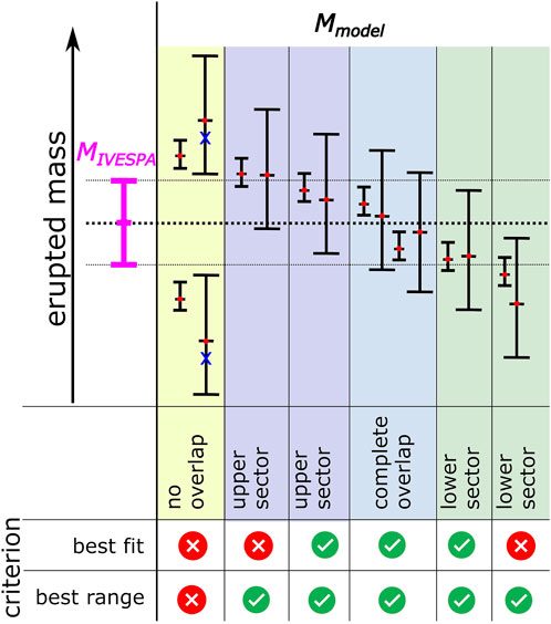
FIGURE 1. Conceptual illustration of the two matching criteria used in this study. To describe the predictive quality of a model (or model combination), the predicted range of the modelled mass Mmodel (examples indicated as black error bars) is compared with the measured range of erupted mass (magenta). Depending on the applied matching criterion, it was tested if a model prediction is successful (green check) or not (red cross). In this study, two criteria were used: “best fit” tests if the best estimate of the model lies within the range of MIVESPA. Two different definitions of best estimates are tested: CMER and FMER. In this illustration, the FMER is indicated by a red dot within the central horizontal black bar. For two examples, also the CMER is marked by blue crosses. The second criterion tests if the ranges of Mmodel and MIVESPA overlap, and is denoted “best range”.
For simplification, we followed the approach introduced by Scollo et al. (2019) and applied plume height corrections only for wind-dominated plumes, using an approximation for the plume radius R suggested by Devenish (2016). Thus Hc was obtained by:
To test the effect of the correction on the outcome, we also computed the “uncorrected” model outcome for Degruyter and Woodhouse, by assuming Hc = h for all cases. The uncorrected model results are marked by the suffix “uncor.”.
The Degruyter model (Eq. 5) and the plume height correction (Eq. 10) require knowledge of the entrainment coefficients. Based on theoretical considerations (e.g., Turner, 1986; Carazzo et al., 2006; Papanicolaou et al., 2008) and experimental findings (Dellino et al., 2014), the radial entrainment coefficient α is known to be ∼0.1. In contrast, the wind entrainment coefficient β is more challenging. The majority of suggested values for β gravitate around 0.5 (Huq and Stewart, 1996; Contini et al., 2011; Michaud-Dubuy et al., 2020), and this is also the value used in the studies of Degruyter and Bonadonna (2012) and Scollo et al. (2019). There are, however, also other studies that suggest different values for β, ranging between 0.1 and 1.0 (Bursik, 2001; Suzuki and Koyaguchi, 2012; Woodhouse et al., 2013). For example, a recent study on the ash plume for Eyjafjallajökull 2010 found that the prediction accuracy of the Degruyter model can be significantly improved when using a value of β = 0.3 (Dürig et al., 2023). Here, we therefore tested two values for β: 0.3 and 0.5 when computing Equations 5, 10. We note that the choice of β in Eq. 10 also influences the results of the Woodhouse model and is therefore always reported along with the results.
2.4 Matching criteria for finding optimal model solutions
To find out which of the tested approaches is most accurate in estimating the MER, we computed the predicted total erupted mass Mmodel, according to:
where t is the duration of the eruptive event. The uncertainties of Mmodel were estimated by using the endmember values (i.e., minimum and maximum values) for h and t, when computing MERmodel and Eq. 12. This results in a range of predicted mass eruption rate MERmodel and predicted erupted mass Mmodel, constrained by the endmembers MERmin and MERmax, and Mmin and Mmax, respectively. Since such an approach is not applicable for the Gudmundsson model (Eq. 4), only the best estimate for MER and Mmodel was computed for this model.
For each eruptive event, the predicted mass is compared to the independently assessed total erupted mass (MIVESPA) from the IVESPA database (Aubry et al., 2021), and the number of matches between Mmodel and MIVESPA is counted. The number of “successful” predictions is then referred to the total number of eruptive events tested, and this ratio is termed “success rate” S. The outcome of this approach is strongly dependent on the mathematical definition of the conditions, under which a prediction provides a match and therefore qualifies as “successful”. In this study we tested two different matching criteria (see Figure 1):
2.4.1 Fitting best estimate (“best fit”)
The simplest matching criterion is to check if the best estimate of the modelled mass Mbest lies within the range of the total erupted mass, thus:
where ΔMIVESPA is the total width of the error bars of erupted mass. The most common approach to obtain the best estimate Mbest is to apply Eq. 12 in combination with the mass eruption rate MERbest that results from plugging in the time-averaged plume height havg as either explicit or implicit model input, depending on whether a plume height correction is applied or not. The commonly defined best estimate of mass eruption rate, here termed as CMER (conventional mass eruption rate), is therefore:
While being simple and straightforward, this definition has a number of drawbacks. It completely neglects the attributed uncertainties in plume heights and duration. Furthermore, due to the highly non-linear correlation between MER and plume height,
An alternative definition of the best MER estimate, which also reflects the MER uncertainties was introduced as FMER (Dürig et al., 2018; 2022; Dioguardi et al., 2020) and is defined by:
In this study we tested the “best fit” matching criterion given in Eq. 13 with both variants of “best mass estimates”, CMER and FMER. In the schematic examples illustrated in Figure 1, Mbest that were computed based on FMER are indicated by a central red dot and black horizontal bar. For two cases, the location of Mbest (CMER) is indicated with blue crosses. These are always situated below Mbest (FMER).
As the only exception, since no comparable definitions for MERmin and MERmax exist for the Gudmundsson model, we used Eq. 4 for the computation of both CMERGud and FMERGud.
2.4.2 Overlapping ranges (“best range”)
The “best range” criterion is fulfilled when the range of the model-predicted mass Mmodel overlaps with the independently measured range of total erupted mass MIVESPA. In contrast to the “best fit” criterion, no definition of best estimate is required. We tested the “best range” criterion for all models, except for the Gudmundsson model, for which no range could be defined for MGud.
2.5 Types of optimized model solutions
In addition to testing the six models individually, we also examined linear combinations of these models. The strategy to combine the models via model weight factors Wmodel is, for example, used by the software REFIR for real-time prediction of the MER (Dürig et al., 2018; Dioguardi et al., 2020). According to this “mixing” strategy, the mass eruption rate is assessed by:
where the sum of the six model weight factors is 1. The range of predicted mass Mmix was computed with Eq. 12, analogue to the procedure for individual models.
A Matlab® script (see Supplementary File S1) was applied that iteratively computes Mmix for all possible combinations of model weight factors with step size 0.01. In a second step, for the selected matching criterion, the weight factor combinations with the highest success rate S were found. In cases where several weight factor solutions exist, we report the combination that i) involves the lowest number of models and ii) prioritizes the simple plume models (Wilson, Sparks, Mastin and, where applicable, Gudmundsson). This prioritization is chosen to minimize the uncertainties that result from combined model uncertainties and from the errors introduced by the additional input parameters required for the explicitly wind-affected models (Degruyter and Woodhouse).
We also examined if S can be further increased by “tailoring” the choice of the model and/or model weight factors to the eruptive conditions. For this purpose, we split the dataset introduced above as “all” into smaller subsets, grouped by:
• Magmatic composition: “basalt”, “andesitic basalt”, “andesite” and “dacite/rhyolite”;
• duration t: the events in the IVESPA database were classified according to their duration into the bins “t<1 h”; “1 h≤t<3 h”; “3 h≤t<12 h”; “12 h≤t<24 h”; “24 h≤t<72 h” and “t ≥72 h”;
• plume type: “buoyancy-dominated”, “intermediate” and “wind-dominated”;
• eruptive style: “magmatic”, “phreatomagmatic”, “unknown” and “phreatic”
• eruptive strength: using the MIVESPA-derived mass eruption rate as grouping variable, together with the bins: “MER<104”; “104≤MER<106”; “106≤MER<107”; “MER≥107”.
All grouping variables were provided by, or computed on the basis of the IVESPA database (Aubry et al., 2021). As illustrated in Figure 2, this results in the following types of model solutions for optimized S:
i. Optimal global model: representing the model that provides the highest success rate for a tested dataset (“all”, “precise” and “control”);
ii. Optimal situation-specific model: model with largest value for S for a specific eruptive condition (e.g., for magmatic eruptions with wind-dominated plumes);
iii. Optimal global mix: combination of model weight factors that provides the largest S for a tested dataset (“all”, “precise” and “control”);
iv. Optimal situation-specific mix: combination of model weight factors that provides the highest success rate for a specific eruptive conditions (e.g., for magmatic eruptions with wind-dominated plumes).
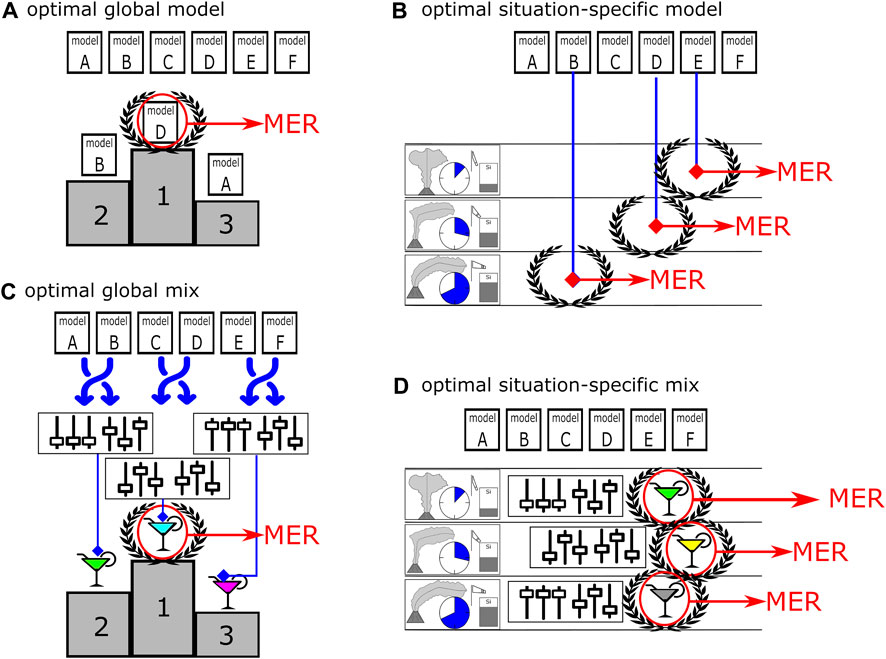
FIGURE 2. Tested types of optimized model solutions: (A) optimal global model is the model with the highest success rate, independent from the eruptive conditions; (B) optimal situation-specific model is the most successful model under a specific eruptive condition. (C) optimal global mix is given by the combination of model weight factors that result in the highest success rate for predicting all tested eruptive events. (D) optimal situation-specific mix is the combination of model weight factors for which the success rate is the highest under specific eruptive conditions. A model or mix marked with a laurel wreath illustrates the most successful solution.
3 Results
3.1 Global model comparisons using individual plume models
The estimates resulting from all tested models are shown in Figure 3 for all tested data subsets. In Figure 3A, the modelled erupted mass is plotted over the measured erupted mass MIVESPA for all 130 events (dataset “all”). This includes cases with unknown MIVESPA errors, for which a 50% uncertainty was assumed. An example of the uncertainties on the observed and simulated total erupted mass for the Wilson model is shown as error bars in Figure 3B. Figures 3C,D are analogue to Figure 3A, but they show the model results for the data subsets “precise” and “control”, respectively. The latter excludes events that were used for the calibration of the models Mastin and Sparks, while the former only includes data points with known mass errors.
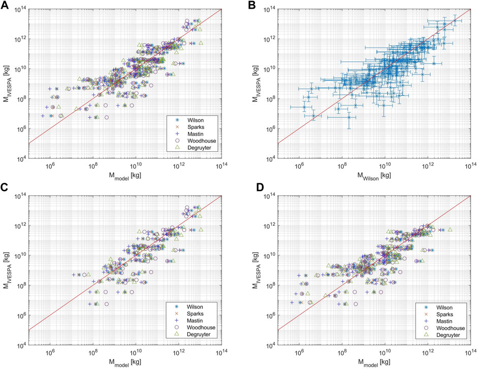
FIGURE 3. Test datasets used in this study: Modelled erupted mass Mmodel is plotted versus the total observed erupted mass MIVESPA as reported by Aubry et al. (2021). Modelled masses are based on the best FMER estimates. The Woodhouse and Degruyter model results were plume-height corrected, using β = 0.5 and β = 0.3, respectively. The red line indicates coordinates of perfect match between modelled and observed mass. (A) Dataset “all” includes all reported IVESPA entries and assumes the MIVESPA error to be 50% for all cases of unknown uncertainties. (B) Wilson model predictions vs. MIVESPA for dataset “all”. The error bars show the wide ranges of uncertainties associated with the observations and model predictions. (C) Model predictions for “precise” data, a subset of dataset “all” that only includes the events with complete information on the MIVESPA uncertainties. (D) Dataset “control” is another subset of dataset “all”, where all events used for the calibration of the Mastin and Sparks models were excluded.
Table 1 presents the success rates S resulting from applying the “best fit” matching criterion to the tested datasets. The values for S range from 7.8% (uncorrected Degruyter model with β = 0.5 and the “precise” subset) to 39.1% (Mastin model with the “precise” subset). When using the FMER definition of Eq. 15 for the “best fit” criterion, the success rates for Sparks, Mastin, uncorrected Woodhouse, plume-height corrected Woodhouse with β = 0.5 and plume-height corrected Degruyter with β = 0.3 are higher than when using the CMER definition of Eq. 14. Using the FMER definition when applying Mastin always leads to a significant increase of S. This finding is in agreement with the optimal MER prediction strategy reported for the different eruptive phases of Eyjafjallajökul 2010 (Dürig et al., 2022) and is further supported by similar results for Mastin with the data subsets “precise” and “control”, where the use of FMER instead of CMER leads to an increase in S from 26.6% to 39.1% and from 28.6% to 30.5%, respectively.
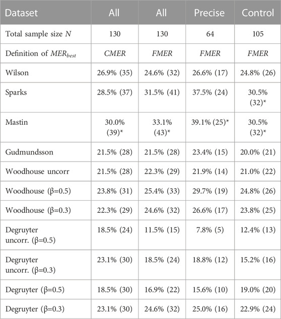
TABLE 1. Success rates S of models tested for three data subsets (“all”, “precise”, and “control”), when applying the “best fit” matching criterion. Numbers in brackets represent the counts of “successful” predictions, using the presented definition of the best MER estimates MERbest. Entries marked by an asterisk represent the highest success rates compared to those from other models.
The success rates S for the “best range” criterion are listed in Table 2. Since the “best range” criterion is less strict than the “best fit” criterion, the success rates are larger, ranging from 54.3% (uncorrected Degruyter with β = 0.5 for dataset “control”) to 84.4% (plume-height corrected Degruyter with β = 0.3 for dataset “precise”). This large variation in success rates demonstrates the importance of applying plume-height corrections, when using the Degruyter model. For both tested matching criteria, the highest success rates are achieved, when a plume height correction is applied, and a wind entrainment coefficient β = 0.3 is assumed. This is in agreement with the findings of Dürig et al. (2023).
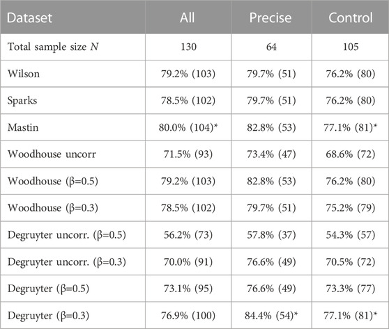
TABLE 2. Success rates S of models tested for three datasets (“all”, “precise”, and “control”), when applying the “best range” matching criterion. Numbers in brackets represent the counts of “successful” predictions. Entries marked by an asterisk represent the highest success rates compared to those from other models.
Also, the success rates of the other wind-affected plume model, Woodhouse, are improved when using corrected plume heights (Table 2). An important difference to the optimal correction for the Degruyter model, however, is that Woodhouse (which does not explicitly depend on β but is implicitly based on the assumption β = 0.9, i.e., for this model the variation of β only affects the top plume height correction) yields higher success rates when using β = 0.5 for the plume height correction with Eq. 10. These outcomes were confirmed for all tested datasets and matching criteria. For the rest of this study, we therefore exclusively focus on model versions with highest success rates, which are the plume height corrected models Degruyter with β = 0.3 and Woodhouse with β = 0.5.
The optimal global model (Figure 2A) depends on the choice of the matching criterion and partly on the tested dataset. When using the “best fit” criterion, Mastin yields the highest success rates for all tested datasets (accompanied by the other empirical 0D model Sparks for dataset “control”). When applying the “best range” criterion, Mastin is the optimal global model for dataset “all” (S = 80.0%), but for the dataset “precise”, Mastin is equally successful to plume-height corrected Woodhouse with β = 0.5 (S = 82.8%), and even excelled by (plume-height corrected) Degruyter with β = 0.3 (S = 84.4%). For dataset “control”, the optimal global models are Mastin and (plume-height corrected) Degruyter with β = 0.3 (S = 77.1%).
3.2 Situation-specific model comparisons
Table 3 shows the success rates of models tested for subsets of the dataset “all” grouped by specified eruptive conditions. For example, when the eruptive events from the IVESPA database are grouped by composition, we find that for basaltic eruptions the optimal situation-specific plume model (i.e., the model with highest S) is Mastin, whereas for eruptions producing andesitic basalts it is Woodhouse. Both models also show the largest success rates in predicting mass eruption rates of dacitic/rhyolitic eruptions. For andesitic eruptions, the most successful plume models are Wilson, Sparks, Mastin and Degruyter with success rates of 75.0%.
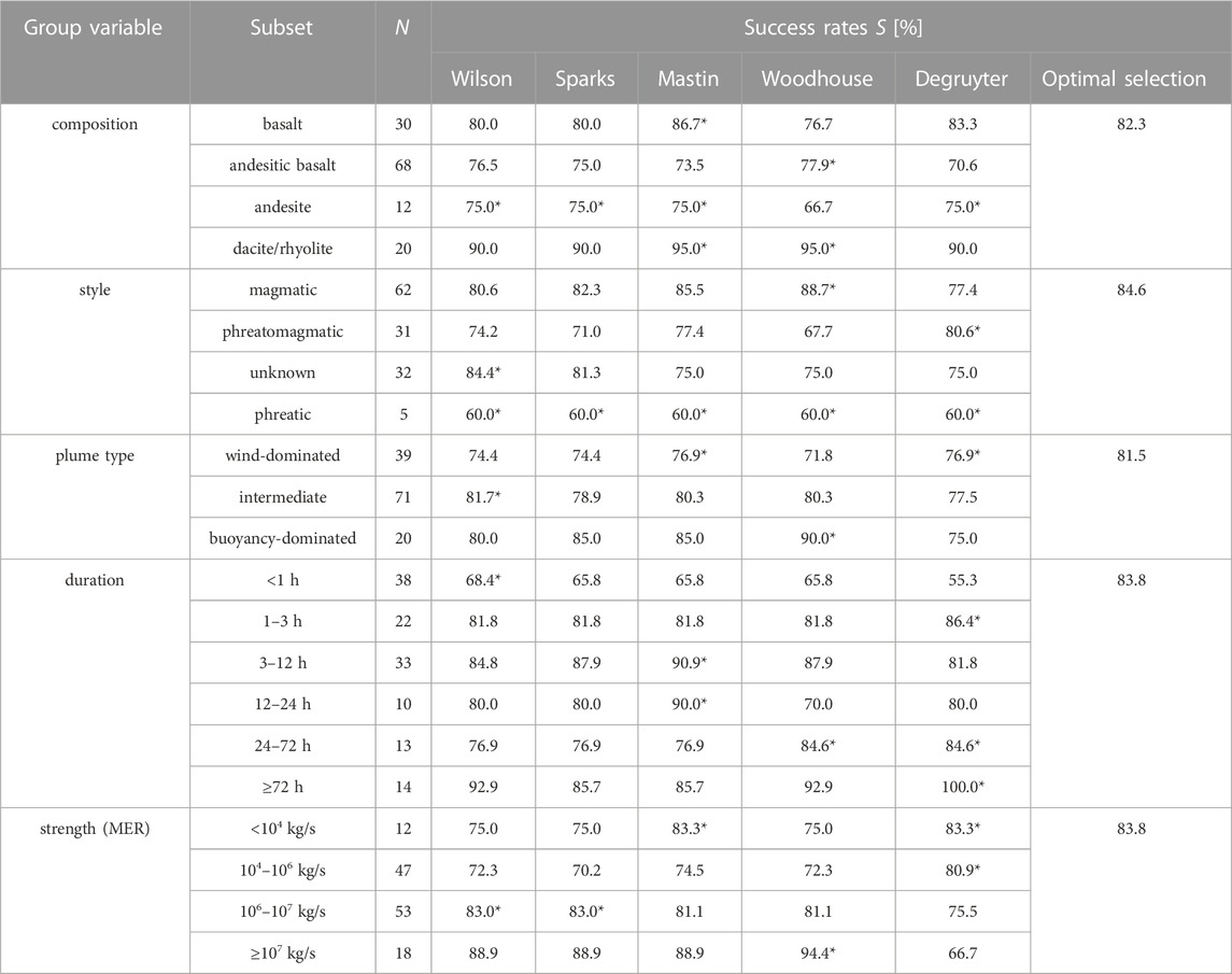
TABLE 3. Success rates S of plume models tested for N eruptive events from dataset “all” under the specified eruptive conditions. The “best range” matching criterion was applied. Optimal situation-specific models with largest S are marked with an asterisk. The rightmost column shows the success rates for selecting the optimal situation-specific model under the tested conditions. The Woodhouse and Degruyter models were computed with plume-height correction and with wind entrainment coefficients β= 0.5 and β= 0.3, respectively.
The success rates listed in Table 3 under “optimal selection” for each group variable were obtained by selecting the optimal situation-specific models and dividing the sum of the accurate predictions by 130, which is the total number of events tested. For example, when selecting Degruyter for wind-dominated plumes, Wilson for intermediate plumes and Woodhouse for buoyancy-dominated plumes, the success rate for this composition-specific optimal model selection strategy is 81.5%, hence slightly higher than the 80% of the global optimal model. Higher gains in S can be achieved, if one of the other tested grouping variables is used as discriminatory eruptive condition for selecting the optimal model. The grouping variable with the highest success rates for the optimal situation-specific model approach turns out to be eruptive style, with a gain in S of 4.6%, compared to the optimal global model predictions. The optimal style-specific models are Woodhouse and Degruyter for magmatic or phreatomagmatic eruptions, respectively, while it is Wilson for eruptions of unknown style. For modelling phreatic eruptions, the success rates appear to be independent from the choice of the model, but the sample size of 5 is too low for any further general inference from this result.
3.3 Optimal global mix solutions
In Table 4, model weight factors W are presented that lead, with Eq. 16, to the highest success rates S for the tested datasets and matching criteria. These weight factors characterize solutions for the optimal global mix (see Figure 2C). For example, for the dataset “all” with “best range” matching criterion, a success rate of 82.3% is obtained for mixing the models with WWilson = 0.20, WSparks = 0.20, WDegruyter = 0.15 and WWoodhouse = 0.45. We note that in contrast to this particular case, the solutions presented are generally not unique, which means that a large numbers of different weight factor solutions can lead to the same given maximum S. The number of solutions is listed as Y in Table 4. For “best fit”, the number of equivalent optimal global mix solutions Y ranges from 3 to 10, while for “best range”, Y ranges from 1 to 97.
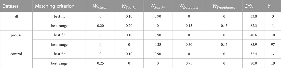
TABLE 4. Optimal global mix solutions: the presented model weight factors W are examples for solutions that result in the highest success rates for the given datasets and matching criteria. The number of all possible optimal solutions found is denoted Y. FMER was used for the “best fit” criterion. The presented results for the models Degruyter and Woodhouse are plume height corrected and used wind-entrainment coefficients of 0.3 and 0.5, respectively.
3.4 Optimal situation-specific mix solutions
Similar to the approach for the optimal situation-specific models (Table 3), it was examined for which grouping variable an optimal selection of weight factors would lead to the highest success rates. Testing dataset “all”, we found that if we distinguish by eruptive style and always select the optimal style-specific combination of weight factors, this results in a success rate of 38.5% with the “best fit” criterion and in 84.6% with the “best range” criterion. The latter value is the same as found for the optimal selection of style-specific models. In other words, within the analyzed step size of 0.01 no weight factor combination was found that would further improve S compared to the solutions listed for optimal style-specific model selection in Table 3. For other grouping variables, however, the combination of various models can lead to higher success rates (all solutions can be found in Supplementary Table S4).
When sorting the dataset by plume type, composition and duration, we find with “best range” optimal situation-specific mix solutions with success rates of 84.6%, 83.8% and 84.6%, respectively. With 85.4%, the highest success rates are obtained when sorting the dataset by eruptive strength, leading to optimal MER-specific mix solutions. An example of optimal composition-specific weight factor combinations is presented in Table 5.
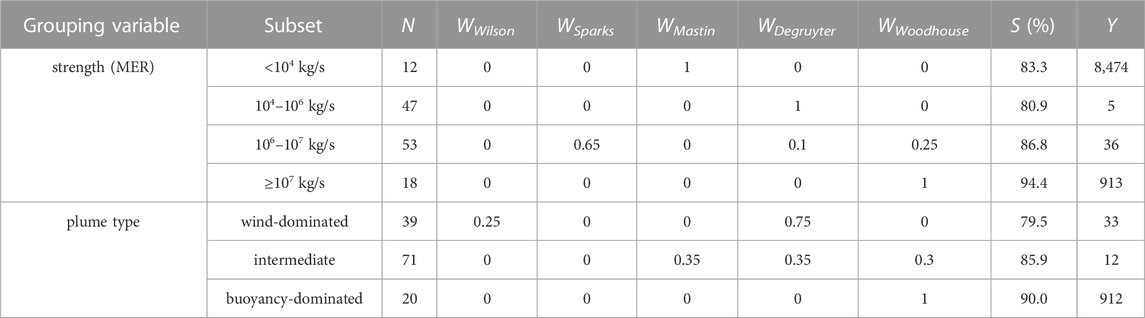
TABLE 5. Optimal situation-specific mix solutions: examples for model weight factors W that result in the highest success rates S for dataset “all” and the given eruptive conditions with “best range” matching criteria. The sample size of the subsets is labelled N, the number of possible optimal solutions is labelled Y. Degruyter and Woodhouse used plume height corrections and wind-entrainment coefficients of 0.3 and 0.5 respectively.
4 Discussion
4.1 Statistical trends for optimized model solutions
The maximum success rates for all tested model solutions, datasets and matching criteria are presented in Figure 4. From the datasets tested, the highest success rates for all model solution types are found for the dataset labelled “precise”. The same observation is made for the success rates of all models (see Tables 1, 2) or mix solutions (see Table 4). Assuming an error of 50% for cases of unknown mass uncertainty increases the sample size, but also introduces an additional source of error, which explains the slightly lower success rates for dataset “all”. The “control” data subset was specifically created to remove any potential bias on the empirical models caused by using the same datasets for testing as was used for calibration. When being tested with the “control” subset for both matching criteria, Mastin remains among the models with largest S. We therefore infer that Mastin can be seen as the “optimal global model” without falling into the trap of circular argumentation. If the aim is to obtain MER predictions without the requirement or knowledge of additional eruptive conditions, applying the Mastin model is a reasonable strategy. This approach is currently applied, e.g., at the London VAAC (Beckett et al., 2020). Our findings are also complementary to (and in good agreement with) findings from a recent study which tested models with the IVESPA data and found empirical models to be more accurate than more complex wind-affected models, including the (in their case uncorrected) Degruyter model (Aubry et al., 2023). While the exact values for S depend on the test dataset used, the general trends of S remain unaffected by the choice of the dataset.
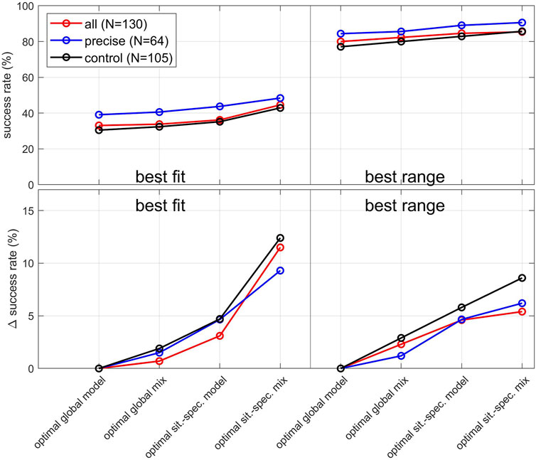
FIGURE 4. Overview of resulting success rates S. In the upper panel, the success rates for all tested MER model solutions are presented for all tested datasets and matching criteria. The lower panel presents the increase in S towards the success rate of the optimal global model, if one of the other model solutions is used instead.
The lower panel of Figure 4 displays the gains in S if optimized model solutions other than the optimal global model is applied. For example, with the “best range” matching criterion, S is increased by 1.2%–2.9% if, instead of simply using Mastin, an optimal combination of models (such as given by Table 4) is globally applied. The “best fit” matching criterion reveals similar gains in S. It is worth noting that for this matching criterion the same weight factor solutions are found for all tested datasets (Table 4): the highest success rates are achieved by using a model combination of 90% Mastin and 10% Sparks. By adding 10% of Sparks to the Mastin model predictions, the success rates of the optimal global mix slightly increased by 0.7%–1.9% (see also Table 1).
A further increase in S can be obtained by using situation-specific model solutions. When applying the “best fit” matching criterion with FMERs, the success rates of optimal situation-specific models range from 16.7% (Wilson, Sparks, Mastin for MER < 104 kg/s) to 65.0% (Sparks for buoyancy-dominated plumes). Mastin qualifies as the optimal situation-specific model for 14 of 21 tested eruptive conditions, Sparks for 6, Woodhouse for 4, and Gudmundsson and Wilson each for 2. If the “best range” matching criterion is used instead (see Table 3), both Mastin and Degruyter are optimal situation-specific models for 8 of 21 tested eruptive conditions, Woodhouse for 6, Wilson for 5, and Sparks for 2. The success rates range from 60% (for phreatic eruptions) to 100% (Degruyter for eruptions with more than 72 h duration). These findings demonstrate that when compared with each other, the tested plume models should not be regarded as generally “worse” or “better”, but rather as being more likely or less likely to provide an accurate MER prediction under given eruptive conditions.
4.2 Examination of “best range” matches
The “best range” matching criterion is a rather lenient one, which is in principle already fulfilled by the slightest overlap between measured and modelled mass. The type of overlap can be further statistically analyzed by distinguishing between three cases, which describes where the modelled mass lies compared to the measured, see Figure 1 for illustration. These are i) cases where the modelled mass is situated in the lower sector of MIVESPA; ii) cases where modelled mass and MIVESPA completely overlap; iii) cases where the modelled mass is situated in the upper sector of the MIVESPA, and therefore is higher than the measured range. The pie diagrams of Figure 5 are an example of such a statistical analysis. The sum of presented success rates for the lower sectors (green), upper sectors (dark blue) and for complete overlap (bright blue) coincide with the success rates for the “best range” criterion for different plume types, as presented in Table 3. For wind-affected plumes, the “best range” success rates of Mastin and Degruyter coincide, but the closer examination of Figure 5 reveals that the matches by Degruyter are more frequently characterized by a complete overlap than for Mastin (49% vs. 38%). Based on this result, it could be inferred that from the two models, Degruyter might have a higher likelihood for successful MER prediction for wind-affected plumes. We note, however, that a large percentage of complete overlap is only meaningful for cases where the error bars of the predicted MER are of comparable size to ΔMIVESPA. In cases where the model uncertainties are far larger, a high overlap is not necessarily an indicator for preciseness and should therefore not be over-interpretated.
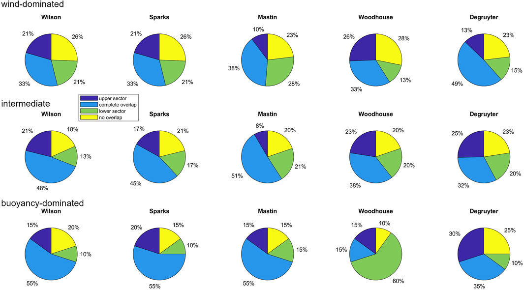
FIGURE 5. Overlap between measured total erupted mass MIVESPA and modelled mass for different plume types.
4.3 Effect of wind on MER predictions
When comparing the success rates for matches with the lower sector with those for matches with the upper sector, Mastin shows with 28% versus 10% a clear prevalence for the former. This indicates a tendency to underestimate the MER for wind-dominated plumes. The same bias is also visible for intermediate plumes (21% vs. 8%) but vanishes for buoyancy dominated plumes (15% vs. 15%). This dependency of prediction quality on windspeed is a phenomenon for simple empirical plume models that is well known from previous studies (Bursik, 2001; Mastin, 2014; Dürig et al., 2022) and was the main reason for the development of wind-affected plume models in the first place (e.g., Bursik, 2001; Degruyter and Bonadonna, 2012; Devenish, 2013; Woodhouse et al., 2013; Mastin, 2014; de’Michieli Vitturi et al., 2015; Folch et al., 2016). It is therefore an interesting side note that for intermediate plumes, Wilson, the simplest (and oldest) of all tested models, is the plume-type specific model with the highest success rates. The complexities of modelling wind-affected plumes are reflected by the fact that the success rates for wind-dominated plumes are significantly lower than for buoyancy-dominated plumes (see Table 3; Figure 5).
4.4 Effect of magmatic composition on model performance
The Gudmundsson model was developed to model the 2010 Eyjafjallajökull eruption, which produced basaltic andesites (Gudmundsson et al., 2012). Surprisingly, for Gudmundsson the “best fit” success rates for basaltic andesitic eruptions are the lowest (16.2%), while it shows its highest success rates for dacites/rhyolites (30%). This might indicate that the model scale factor kI is less dependent on composition than on other parameters, such as wind conditions and eruptive style.
The other two empirical models (Sparks and Mastin) are trained on datasets where basaltic eruptions are arguably underrepresented. However, we do not observe any significantly lower success rates for eruptive events of basaltic composition (Table 3). This finding speaks against a significant influence of a compositional bias in the underlying datasets.
4.5 Effect of eruptive style on MER predictions
The optimal style-specific models found were Woodhouse for magmatic and Degruyter for phreatomagmatic eruptions. Phreatomagmatic eruptions are characterized by a much larger water content in the plume, which significantly changes the heat capacity of the mixture (Sparks et al., 1997; Degruyter and Bonadonna, 2012). Unlike magmatic eruptions, for which the source of energy is provided by expanding gas, phreatomagmatic eruptions are driven by explosive molten fuel-coolant interaction (MFCI) (Zimanowski et al., 2015; White and Valentine, 2016). MFCI is a thermohydraulic mechanism that converts the heat of the magmatic melt into shock waves and mechanical stress, which drives the fragmentation of the melt and leads to the generation of ash particles (Dürig et al., 2012b; Dürig and Zimanowski, 2012; Dürig et al., 2020). The energy expended for both vaporization of the water and fragmentation of the melt results in a significant cooling of the fragmented melt (Spitznagel et al., 2013; Moitra et al., 2020). Consequently, the temperature of tephra in phreatomagmatic plumes is expected to be considerably lower than for ash columns resulting from magmatic explosions. Another important difference between phreatomagmatic and magmatic eruptions is the abundance of fine “interactive” ash particles in phreatomagmatic plumes that together with agglomeration effects, particle aggregation processes and the presence of fragmented host rock lead to differences in grain size distributions and the plume’s bulk density (Zimanowski et al., 2003; Dürig et al., 2012a; Dürig et al., 2020; Andrews et al., 2014; White and Valentine, 2016). All these factors influence the plume dynamics, which might not only explain why the models’ S are so different for both plume types, but also why the success rates for magmatic eruptions are generally higher (with a maximum “best range” S of 88.7%, see Table 3) than for the more varied phreatomagmatic eruptions (with a maximum S of 80.6%).
The results in Table 3 also show that a correct identification of the eruptive condition is crucial for an effective use of the situation-specific model strategies, because a misclassification would lead to significantly lower success rates. For example, let’s assume that a phreatomagmatic eruption is wrongly identified as magmatic. If the optimal style-specific model for magmatic eruptions (Woodhouse) is applied to phreatomagmatic eruptions, the success rates are not as expected (88.7%) but only 67.7%, which is lower than for any other of the tested models. Conversely, Degruyter has, with 77.4%, the lowest success rates of all models for magmatic eruptions. In both cases, the optimal global model (Mastin) yields higher success rates, which means that the situation-specific modelling strategy was not helpful, but in fact harmful for optimizing the forecast quality. This phenomenon is observed for all of the other grouping variables and datasets tested. We therefore conclude that the strategies of optimal situation-specific model (or optimal situation-specific mix) solutions should only be applied if the eruptive condition used for tailoring the modelling strategy is well known. Otherwise, it is highly recommended to fall back on the optimal global mix or optimal global model, which are both easier and more accurate than the situation-specific solutions.
4.6 Suggested quality optimization strategy for MER forecast
The only situation-specific mix solutions that have shown to be more successful than the optimal eruptive style-specific model solution are the MER-specific solutions (see example in Table 5). Using the MER for the decision of choosing the weight factors is, however, not expected to always be a very practical procedure, given that MER is the unknown parameter which we aim to simulate with the models. The only viable way for the MER-specific mix strategy to succeed is by applying an iterative procedure. Based on these considerations, we designed the procedure displayed in the flow chart in Figure 6 to forecast the MER in a real-time plume monitoring scenario with highest accuracy. First it is checked if meteorological data (required for the wind-affected plume models Woodhouse and Degruyter) are available. If this is not the case, we suggest using the optimal global model for MER forecast (i.e., Mastin). If meteorological data are available, in a next step the MER category of the current eruption is classified based on a preliminary MER estimated with the optimal global mix (Table 4).
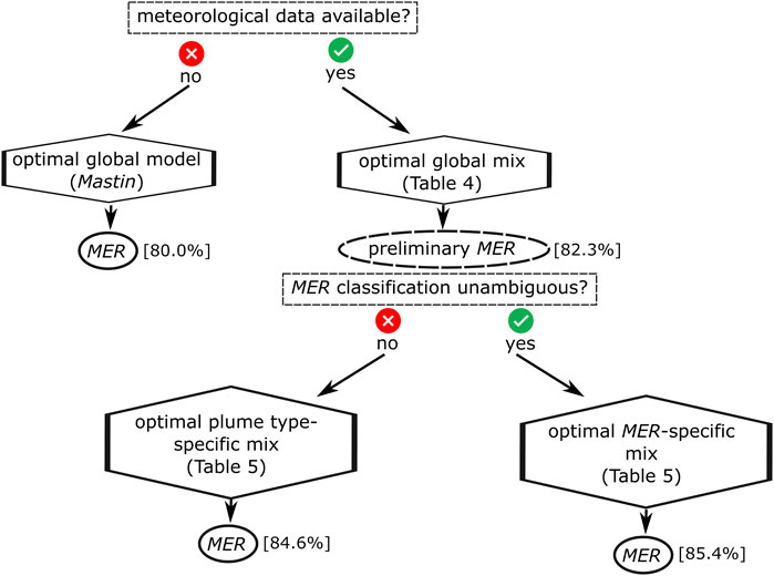
FIGURE 6. Decision tree to select the optimal MER modelling strategy. Values in square brackets indicate the success rates found with dataset “all” and “best range” matching criterion. The optimal choice of the modelling approach depends on the availability and quality of real-time information.
Examples for eruptions of unambiguous strengths are eruptions with a MER << 104 kg/s, MER >>107 kg/s or not significantly wind-affected eruptions with a mass eruption rate that is well limited within 104 kg/s and 106 kg/s. Based on the MER classification, the appropriate weight factors should be selected according to Table 5. Interestingly, for eruptions with MER <104 kg/s, Mastin has shown to be the optimal model, despite the fact that such weak eruptions were underrepresented in the dataset underlying this model (Mastin et al., 2009; Mastin, 2014). When it is not possible to constrain the category of eruptive strength with sufficient certainty, it is better to choose another grouping variable, despite the slightly lower success rates.
The optimal situation-specific mix solutions grouped by plume type, eruptive style and duration all have identical success rates of 84.6% (Supplementary Table S4). From these parameters, duration is realistically the least practical one for real-time monitoring purposes, due to its low predictability. Since a plume-type classification has to be conducted anyway to apply the necessary plume height corrections for the wind-affected plume models, we suggest using optimal situation-specific mix solutions tailored for plume-types. Suitable model weight factor settings are presented in Table 5.
4.7 IVESPA dataset uncertainties
The plume heights used for this study are taken from the IVESPA database, which were acquired by a multitude of different methods, including visual observations and measurements with radar, lidar or satellites (Aubry et al., 2021). This bears a potential of errors, since it has been shown that the MER prediction quality is dependent on the method of plume height source (Aubry et al., 2023). Future studies could therefore focus on subsets of dataset “all” that only contain events with known plume heights from one measurement technique. A similar approach was followed, for example, in recent studies on Eyjafjallajökull 2010 (Dürig et al., 2022) and Etna (Mereu et al., 2023). As demonstrated for the 2010 Eyjafjallajökull eruption, the temporal resolution of the plume height average has a significant impact on the outcome of the modelled MER (Dürig et al., 2022). All plume height values from IVESPA are averaged over the total duration of the eruptions, a parameter which itself varies considerably. While a single average value for plume height can be sufficient to constrain a rather short-lived event of, for example, less than 6 h duration, it is less useful for quantifying the strengths of long-lived eruptions that feature changing source and atmospheric conditions. The fact that we found different results for different durations reflects this effect.
The weather data from IVESPA used in our study are based on ERA5, which is probably the best global product available, but due to effect of necessary interpolation from grid points of the global model to the location of the volcano, there can be significant errors in, e.g., windspeed. However, it is expected that this error is small in comparison to the larger uncertainties introduced from plume height and duration.
4.8 Outlier events
Seven out of the 130 eruptive events from dataset “all” were identified as “outlier events” (see Supplementary Table S5). These are events for which the simulated mass never meets the “best range” matching criterion with the range of the measured erupted mass (MIVESPA), regardless of the type of optimized model solutions. All identified events are also part of the “precise” data subset.
In the following, the outlier events are listed and potential aggravating factors and circumstances are discussed that might have complicated the predictability of these outlier events:
(i) Redoubt Alaska 1989 December 19: this was a very short-lived phreatomagmatic eruption, which lasted only 9 min (Miller and Chouet, 1994). All tested models tested assume a steady plume, which is fed by a stream of ash and gas with a constant MER (Morton et al., 1956; Sparks et al., 1997). This assumption is not suitable for eruptions of very short duration (for example, when the ascent time of the ash column is in the same order of magnitude as the total duration of the eruption), or for pulsatile behavior with sufficiently long repose times (Dürig et al., 2015b). Therefore, all models underestimate the MER.
(ii) Soufrière Hills Montserrat 1997 September 26: this magmatic eruption lasted 60 min and was therefore also short-lived (Bonadonna and Costa, 2012). We suggest that the steady-state condition is not achieved and might be the main reason why none of the tested model solutions correctly predict the MER.
(iii) Merapi Indonesia 2010 November 4: this magmatic eruption lasted 36 h. It started with a climactic explosion, followed by intermittent explosions and featured source conditions of varied eruptive activity. An additional complicating circumstance was the observed occurrence of syn-eruptive pyroclastic flows that might have contributed to the rising dynamics of the eruption column (all information from: Surono et al., 2012). It is comprehensible that using only one value (the plume height averaged over the 36 h time interval) to describe the source conditions of this complex sequence of events is probably too simplistic to be able to accurately estimate the MER.
(iv) Eyjafjallajökull Iceland 2010 April 14–16: The first explosive phase of this eruption was driven by phreatomagmatic explosions and lasted 72 h (Dellino et al., 2012). All tested model solutions tested underestimate the erupted mass. It could be argued that the values given in the IVESPA database for MIVESPA (Aubry et al., 2021) might be too high: the total erupted mass reported in IVESPA also includes the tephra transported by jökulhaups. If, however, only the airborne tephra is considered, MIVESPA reduces from 1.3·1011 kg to 9.8·1010 kg (Table 1 in Gudmundsson et al., 2012), which matches all tested optimal situation-specific model solutions. This indicates that the water transported ash did not contribute to the formation of the plume, because it was trapped in the overlying glacier ice. We note that the lower value was also used as measured erupted mass in recent case studies on Eyjafjallajökull 2010 to investigate the effect of timing and wind on simple plume models (Dürig et al., 2022) and to examine plume height correction strategies for wind-affected plume models (Dürig et al., 2023).
(v) Cotopaxi Ecuador 2015, first phase: this phreatic event is with a (deposit-computed) MER of 3.1·103 kg/s (Bernard et al., 2016) within the lowest 10th percentile in terms of eruptive strength when compared to all events listed in IVESPA. The combination of eruptive style and the fact that it classifies as a very weak eruption might explain why all tested model solutions overestimate the total erupted mass.
(vi) Etna Italy 2016 May 21: based on fallout measurements, this eruption was an extremely weak eruption with a MER of only 0.7·103 kg/s, which puts this event in the lowest 5th percentile of all eruptions listed in IVESPA in terms of eruptive strength. The eruption took place at very windy conditions, with recorded windspeeds of 23.3 m/s on average. Furthermore, syn-eruptive lava flows and lava fountains were reported (all information from: Edwards et al., 2018). It is known that empirical plume models tend to underestimate the MER from wind-affected plumes (Bursik, 2001; Mastin, 2014; Dürig et al., 2022). We would therefore expect that modelling the MER of this eruption would struggle with an underestimation bias. However, we observe the opposite: all model solutions systematically overestimate the total erupted mass. We therefore infer that the syn-eruptive lava flows and lava fountains, which are probably not controlled by the same fragmentation processes and physics of brittle magma fragmentation observed in explosive volcanism (La Spina et al., 2021), might have played a significant role in contributing to the total heat budget that drove the ash plume in a sort of “hotplate effect”.
(vii) Chaitén Chile 2008 alpha layer: this rhyolitic eruptive event took place under very variable wind intensities and with relatively large average windspeeds of 16.2 m/s (Folch et al., 2008). The plume was issued from two vents, featuring a plume height of initially over 20 km, later dropping to 11–17 km (Folch et al., 2008; Major and Lara, 2013). The combination of the large variability in wind intensity and plume height, and the unusual dual vent configuration, might explain why it is so challenging to model this eruptive event.
4.9 Plume height as proxy for MER
The six models examined in this study have the advantage that they use with plume height h as main input parameter, which is relatively easy to obtain, despite the important limitation that the value can be dependent on the method of measurement itself (Dürig et al., 2022; Aubry et al., 2023). Relatively small errors in h, however, result in considerable uncertainties in MER, often covering one or more orders of magnitude (see Figure 3), due to the exponential relationship between MER and h. Applying the discussed strategies of mixing different plume height-based models cannot compensate for this effect, because it is intrinsic to all models tested.
Approaches for real-time MER forecast that do not use plume-height exist, but they require i) more sophisticated instruments and ii) knowledge of additional parameters that are often difficult to acquire. For example, MER prediction by infra-sound requires detailed information on the vent geometry (Johnson and Ripepe, 2011; Ripepe et al., 2013), without which the uncertainties are considerable (Dürig et al., 2015b). Other methods, like electric field measurements are still in development and need further calibration and testing under different eruptive conditions (Büttner et al., 2000; Calvari et al., 2012).
If instruments and necessary input data are available, the most promising strategy to better constrain the MER is to combine several independent prediction methods (e.g., estimates from infra-sound with the presented plume-height based 0D model forecasts).
5 Conclusion
In the present study we empirically examined the prediction accuracy of MER modelling strategies that are based on six plume models. Using three different subsets of the IVESPA database (Aubry et al., 2021), which contains independently obtained eruption source parameters of up to 130 eruptive events, we introduced two different matching criteria and tested for each case if the total erupted mass derived from fallout measurements fits the predicted erupted mass. The counts of matching predictions were summarized and referred to the number of compared events, resulting in percentage success rates S. Under the hypothesis that the likelihood of accurately predicting the MER of a future eruptive event is mirrored by the success rates, we present ways to optimize the discussed modelling strategies. It was shown that computing FMER (Eq. (15)) instead of using the averaged plume heights leads to higher success rates with the “best fit” matching criterion. The success rates of wind-affected plume models are significantly increased if a plume height correction according to Eq. 10 is applied. For the Degruyter model (Degruyter and Bonadonna, 2012) success rates were significantly higher when using a wind entrainment rate β of 0.3. The Woodhouse model (Woodhouse et al., 2013), however, shows higher success rates for β= 0.5.
According to our results, the expected accuracy of the modelling strategy depends on the amount (and quality) of volcanological, geological, geochemical and meteorological information that is available for the monitored eruption. If no real-time information other than plume height is available from the tested models, we suggest choosing the Mastin model (Mastin et al., 2009), as it has shown the highest success rates.
It was shown that instead of simply relying on the application of one plume model for all situations, the accuracy of real-time MER forecast could be further increased by a situation-specific selection of plume models or/and by mixing the different models by means of model weight factors. Based on these considerations, we introduce a decision tree that is designed to advice stake holders in their choice of the optimal modelling strategy (see Figure 6), when monitoring an eruption in real-time, e.g., with the monitoring software REFIR (Dürig et al., 2018; Dioguardi et al., 2020).
Data availability statement
The original contributions presented in the study are included in the article/Supplementary Material, further inquiries can be directed to the corresponding author.
Author contributions
TD, LS, and FD contributed to conception and design of the study. LS and TD coded the Matlab scripts used for the analysis presented in this study. TD conducted the statistical analysis and wrote the first draft of the manuscript. LS wrote sections of the manuscript. All authors contributed to the article and approved the submitted version.
Funding
TD was supported by the Icelandic Research Fund (Rannís), grant Nr. 206527-051. FD was supported by the RETURN Extended Partnership and received funding from the European Union NextGenerationEU (National Recovery and Resilience Plan–NRRP, Mission 4, Component 2, Investment 1.3—D.D. 1243 2/8/2022, PE0000005). This work contributes to project MAXI-Plume, supported by the Icelandic Research Fund (Rannís), grant Nr. 206527-051.
Acknowledgments
We thank Dr. Valerio Acocella and Luis E. Lara for editing, and Dr. Jorge E. Romero and an reviewer for their constructive comments that helped improve the manuscript.
Conflict of interest
The authors declare that the research was conducted in the absence of any commercial or financial relationships that could be construed as a potential conflict of interest.
Publisher’s note
All claims expressed in this article are solely those of the authors and do not necessarily represent those of their affiliated organizations, or those of the publisher, the editors and the reviewers. Any product that may be evaluated in this article, or claim that may be made by its manufacturer, is not guaranteed or endorsed by the publisher.
Supplementary material
The Supplementary Material for this article can be found online at: https://www.frontiersin.org/articles/10.3389/feart.2023.1250686/full#supplementary-material
References
Andrews, R. G., White, J. D. L., Dürig, T., and Zimanowski, B. (2014). Discrete blasts in granular material yield two-stage process of cavitation and granular fountaining. Geophys. Res. Lett. 41, 422–428. doi:10.1002/2013GL058526
Aubry, T. J., Jellinek, A. M., Carazzo, G., Gallo, R., Hatcher, K., and Dunning, J. (2017). A new analytical scaling for turbulent wind-bent plumes: comparison of scaling laws with analog experiments and a new database of eruptive conditions for predicting the height of volcanic plumes. J. Volcanol. Geotherm. Res. 343, 233–251. doi:10.1016/j.jvolgeores.2017.07.006
Aubry, T. J., Engwell, S., Bonadonna, C., Carazzo, G., Scollo, S., Van Eaton, A. R., et al. (2021). The independent volcanic eruption source parameter archive (IVESPA, version 1.0): A new observational database to support explosive eruptive column model validation and development. J. Volcanol. Geotherm. Res. 417, 107295. doi:10.1016/j.jvolgeores.2021.107295
Aubry, T. J., Engwell, S., Bonadonna, C., Mastin, L. G., Carazzo, G., Van Eaton, A. R., et al. (2023). New insights into the relationship between mass eruption rate and volcanic column height based on the IVESPA dataset. Geophys. Res. Lett. 50, e2022GL102633. doi:10.1029/2022GL102633
Bear-Crozier, A., Pouget, S., Bursik, M., Jansons, E., Denman, J., Tupper, A., et al. (2020). Automated detection and measurement of volcanic cloud growth: towards a robust estimate of mass flux, mass loading and eruption duration. Nat. Hazards 101, 1–38. doi:10.1007/s11069-019-03847-2
Beckett, F. M., Witham, C. S., Hort, M. C., Stevenson, J. A., Bonadonna, C., and Millington, S. C. (2015). Sensitivity of dispersion model forecasts of volcanic ash clouds to the physical characteristics of the particles. J. Geophys. Res. Atmos. 120, 11636–11652. doi:10.1002/2015JD023609
Beckett, F. M., Witham, C. S., Leadbetter, S. J., Crocker, R., Webster, H. N., Hort, M. C., et al. (2020). Atmospheric dispersion modelling at the London VAAC: A review of developments since the 2010 Eyjafjallajökull volcano ash cloud. Atmos. (Basel) 11, 352. doi:10.3390/atmos11040352
Bernard, B., Battaglia, J., Proaño, A., Hidalgo, S., Vásconez, F., Hernandez, S., et al. (2016). Relationship between volcanic ash fallouts and seismic tremor: quantitative assessment of the 2015 eruptive period at Cotopaxi volcano, Ecuador. Bull. Volcanol. 78, 80. doi:10.1007/s00445-016-1077-5
Bonadonna, C., and Costa, A. (2012). Estimating the volume of tephra deposits: A new simple strategy. Geology 40, 415–418. doi:10.1130/G32769.1
Bonadonna, C., Pistolesi, M., Cioni, R., Degruyter, W., Elissondo, M., and Baumann, V. (2015). Dynamics of wind-affected volcanic plumes: the example of the 2011 Cordón Caulle eruption, Chile. J. Geophys. Res. Solid Earth 120, 2242–2261. doi:10.1002/2014JB011478
Bonadonna, C., Cioni, R., Costa, A., Druitt, T., Phillips, J., Pioli, L., et al. (2016). MeMoVolc report on classification and dynamics of volcanic explosive eruptions. Bull. Volcanol. 78, 84. doi:10.1007/s00445-016-1071-y
Bursik, M. (2001). Effect of wind on the rise height of volcanic plumes. Geophys. Res. Lett. 28, 3621–3624. doi:10.1029/2001GL013393
Büttner, R., Zimanowski, B., and Röder, H. (2000). Short-time electrical effects during volcanic eruption: experiments and field measurements. J. Geophys. Res. Solid Earth 105, 2819–2827. doi:10.1029/1999JB900370
Calvari, S., Büttner, R., Cristaldi, A., Dellino, P., Giudicepietro, F., Orazi, M., et al. (2012). The 7 September 2008 Vulcanian explosion at Stromboli volcano: multiparametric characterization of the event and quantification of the ejecta. J. Geophys. Res. Solid Earth 117, B05201. doi:10.1029/2011JB009048
Carazzo, G., Kaminski, E., and Tait, S. (2006). The route to self-similarity in turbulent jets and plumes. J. Fluid Mech. 547, 137. doi:10.1017/S002211200500683X
Carey, S., and Sparks, R. S. J. (1986). Quantitative models of the fallout and dispersal of tephra from volcanic eruption columns. Bull. Volcanol. 48, 109–125. doi:10.1007/BF01046546
Cerminara, M., Esposti Ongaro, T., Valade, S., and Harris, A. J. L. (2015). Volcanic plume vent conditions retrieved from infrared images: A forward and inverse modeling approach. J. Volcanol. Geotherm. Res. 300, 129–147. doi:10.1016/j.jvolgeores.2014.12.015
Cerminara, M., Esposti Ongaro, T., and Berselli, L. C. (2016). ASHEE-1.0: a compressible, equilibrium–eulerian model for volcanic ash plumes. Geosci. Model Dev. 9, 697–730. doi:10.5194/gmd-9-697-2016
Contini, D., Donateo, A., Cesari, D., and Robins, A. G. (2011). Comparison of plume rise models against water tank experimental data for neutral and stable crossflows. J. Wind Eng. Ind. Aerodyn. 99, 539–553. doi:10.1016/j.jweia.2011.02.003
Costa, A., Suzuki, Y. J., Cerminara, M., Devenish, B. J., Ongaro, T. E., Herzog, M., et al. (2016). Results of the eruptive column model inter-comparison study. J. Volcanol. Geotherm. Res. 326, 2–25. doi:10.1016/j.jvolgeores.2016.01.017
Dacre, H. F., Grant, A. L. M., Hogan, R. J., Belcher, S. E., Thomson, D. J., Devenish, B. J., et al. (2011). Evaluating the structure and magnitude of the ash plume during the initial phase of the 2010 Eyjafjallajökull eruption using lidar observations and NAME simulations. J. Geophys. Res. 116, D00U03. doi:10.1029/2011JD015608
Davis, J. C. (2002). in Statistics and data analysis in geology. Editor M. Gerber 3rd edition (New York; Chichester; Brisbane: John Wiley & Sons).
de’Michieli Vitturi, M., Neri, A., and Barsotti, S. (2015). PLUME-MoM 1.0: A new integral model of volcanic plumes based on the method of moments. Geosci. Model Dev. 8, 2447–2463. doi:10.5194/gmd-8-2447-2015
Degruyter, W., and Bonadonna, C. (2012). Improving on mass flow rate estimates of volcanic eruptions. Geophys. Res. Lett. 39, 1–6. doi:10.1029/2012GL052566
Dellino, P., Gudmundsson, M. T., Larsen, G., Mele, D., Stevenson, J. A., Thordarson, T., et al. (2012). Ash from the Eyjafjallajökull eruption (Iceland): fragmentation processes and aerodynamic behavior. J. Geophys. Res. Solid Earth 117, B00C04. doi:10.1029/2011JB008726
Dellino, P., Dioguardi, F., Mele, D., D’Addabbo, M., Zimanowski, B., Büttner, R., et al. (2014). Volcanic jets, plumes, and collapsing fountains: evidence from large-scale experiments, with particular emphasis on the entrainment rate. Bull. Volcanol. 76, 834. doi:10.1007/s00445-014-0834-6
Devenish, B. J. (2013). Using simple plume models to refine the source mass flux of volcanic eruptions according to atmospheric conditions. J. Volcanol. Geotherm. Res. 256, 118–127. doi:10.1016/j.jvolgeores.2013.02.015
Devenish, B. J. (2016). Estimating the total mass emitted by the eruption of Eyjafjallajökull in 2010 using plume-rise models. J. Volcanol. Geotherm. Res. 326, 114–119. doi:10.1016/j.jvolgeores.2016.01.005
Dioguardi, F., Dürig, T., Engwell, S. L., Gudmundsson, M. T., and Loughlin, S. C. (2016). “Investigating source conditions and controlling parameters of explosive eruptions: some experimental-observational- modelling case studies,” in Updates in Volcanology - from volcano modelling to volcano geology. Editor K. Németh (Rijeka: InTech). doi:10.5772/63422
Dioguardi, F., Beckett, F., Dürig, T., and Stevenson, J. A. (2020). The impact of eruption source parameter uncertainties on ash dispersion forecasts during explosive volcanic eruptions. J. Geophys. Res. Atmos. 125, e2020JD032717. doi:10.1029/2020JD032717
Dürig, T., and Zimanowski, B. (2012). “Breaking news” on the formation of volcanic ash: fracture dynamics in silicate glass. Earth Planet. Sci. Lett. 335, 1–8. doi:10.1016/j.epsl.2012.05.001
Dürig, T., Mele, D., Dellino, P., and Zimanowski, B. (2012a). Comparative analyses of glass fragments from brittle fracture experiments and volcanic ash particles. Bull. Volcanol. 74, 691–704. doi:10.1007/s00445-011-0562-0
Dürig, T., Sonder, I., Zimanowski, B., Beyrichen, H., and Büttner, R. (2012b). Generation of volcanic ash by basaltic volcanism. J. Geophys. Res. Solid Earth 117. doi:10.1029/2011JB008628
Dürig, T., Gudmundsson, M. T., and Dellino, P. (2015a). Reconstruction of the geometry of volcanic vents by trajectory tracking of fast ejecta - the case of the Eyjafjallajökull 2010 eruption (Iceland). Earth, Planets Sp. 67, 64. doi:10.1186/s40623-015-0243-x
Dürig, T., Gudmundsson, M. T., Karmann, S., Zimanowski, B., Dellino, P., Rietze, M., et al. (2015b). Mass eruption rates in pulsating eruptions estimated from video analysis of the gas thrust-buoyancy transition—A case study of the 2010 eruption of Eyjafjallajökull, Iceland. Earth, Planets Sp. 67, 180. doi:10.1186/s40623-015-0351-7
Dürig, T., Gudmundsson, M. T., Dioguardi, F., Woodhouse, M., Björnsson, H., Barsotti, S., et al. (2018). REFIR- A multi-parameter system for near real-time estimates of plume-height and mass eruption rate during explosive eruptions. J. Volcanol. Geotherm. Res. 360, 61–83. doi:10.1016/j.jvolgeores.2018.07.003
Dürig, T., White, J. D. L., Murch, A. P., Zimanowski, B., Büttner, R., Mele, D., et al. (2020). Deep-sea eruptions boosted by induced fuel–coolant explosions. Nat. Geosci. 13, 498–503. doi:10.1038/s41561-020-0603-4
Dürig, T., Ross, P.-S., Dellino, P., White, J. D. L., Mele, D., and Comida, P. P. (2021). A review of statistical tools for morphometric analysis of juvenile pyroclasts. Bull. Volcanol. 83, 79. doi:10.1007/s00445-021-01500-0
Dürig, T., Gudmundsson, M. T., Ágústsdóttir, T., Högnadóttir, T., and Schmidt, L. S. (2022). The effect of wind and plume height reconstruction methods on the accuracy of simple plume models — A second look at the 2010 Eyjafjallajökull eruption. Bull. Volcanol. 84, 33. doi:10.1007/s00445-022-01541-z
Dürig, T., Gudmundsson, M. T., Dioguardi, F., and Schmidt, L. S. (2023). Quantifying the effect of wind on volcanic plumes: implications for plume modeling. J. Geophys. Res. Atmos. 128. doi:10.1029/2022JD037781
Edwards, M. J., Pioli, L., Andronico, D., Scollo, S., Ferrari, F., and Cristaldi, A. (2018). Shallow factors controlling the explosivity of basaltic magmas: the 17–25 May 2016 eruption of Etna Volcano (Italy). J. Volcanol. Geotherm. Res. 357, 425–436. doi:10.1016/j.jvolgeores.2018.05.015
Esposti Ongaro, T., Cavazzoni, C., Erbacci, G., Neri, A., and Salvetti, M. V. (2007). A parallel multiphase flow code for the 3D simulation of explosive volcanic eruptions. Parallel comput. 33, 541–560. doi:10.1016/j.parco.2007.04.003
Folch, A., Jorba, O., and Viramonte, J. (2008). Volcanic ash forecast – application to the May 2008 Chaitén eruption. Nat. Hazards Earth Syst. Sci. 8, 927–940. doi:10.5194/nhess-8-927-2008
Folch, A., Costa, A., and Macedonio, G. (2016). FPLUME-1.0: an integral volcanic plume model accounting for ash aggregation. Geosci. Model Dev. 9, 431–450. doi:10.5194/gmd-9-431-2016
Gouhier, M., Eychenne, J., Azzaoui, N., Guillin, A., Deslandes, M., Poret, M., et al. (2019). Low efficiency of large volcanic eruptions in transporting very fine ash into the atmosphere. Sci. Rep. 9, 1449. doi:10.1038/s41598-019-38595-7
Grindle, T. J., and Burcham, F. W. (2002). Even minor volcanic ash encounters can cause major damage to aircraft. ICAO J. 57, 12–14.
Gudmundsson, M. T., Thordarson, T., Höskuldsson, Á., Larsen, G., Björnsson, H., Prata, F. J., et al. (2012). Ash generation and distribution from the April-May 2010 eruption of Eyjafjallajökull, Iceland. Sci. Rep. 2, 572. doi:10.1038/srep00572
Harris, A. J. L., Delle Donne, D., Dehn, J., Ripepe, M., and Worden, A. K. (2013). Volcanic plume and bomb field masses from thermal infrared camera imagery. Earth Planet. Sci. Lett. 365, 77–85. doi:10.1016/j.epsl.2013.01.004
Harris, A. (2013). Thermal remote sensing of active volcanoes: A user’s manual. New York: Cambridge University Press. Available at: https://books.google.de/books?id=xY4oYzbH0ooC.
Hersbach, H., Bell, B., Berrisford, P., Biavati, G., Horányi, A., Muñoz Sabater, J., et al. (2018). ERA5: Fifth generation of ECMWF atmospheric reanalyses of the global climate. Copernicus Clim. Chang. Serv. Clim. Data Store CDS (accessedFebruary17, 2021).
Hersbach, H., Bell, B., Berrisford, P., Hirahara, S., Horányi, A., Muñoz-Sabater, J., et al. (2020). The ERA5 global reanalysis. Q. J. R. Meteorol. Soc. 146, 1999–2049. doi:10.1002/qj.3803
Hewett, T. A., Fay, J. A., and Hoult, D. P. (1971). Laboratory experiments of smokestack plumes in a stable atmosphere. Atmos. Environ. 5, 767–789. doi:10.1016/0004-6981(71)90028-X
Hochfeld, I., Hort, M., Schwalbe, E., and Dürig, T. (2022). Eruption dynamics of Anak Krakatau volcano (Indonesia) estimated using photogrammetric methods. Bull. Volcanol. 84, 73. doi:10.1007/s00445-022-01579-z
Huq, P., and Stewart, E. J. (1996). A laboratory study of buoyant plumes in laminar and turbulent crossflows. Atmos. Environ. 30, 1125–1135. doi:10.1016/1352-2310(95)00335-5
Johnson, J. B., and Ripepe, M. (2011). Volcano infrasound: A review. J. Volcanol. Geotherm. Res. 206, 61–69. doi:10.1016/j.jvolgeores.2011.06.006
Kienle, J., Kyle, P. R., Self, S., Motyka, R. J., and Lorenz, V. (1980). Ukinrek Maars, Alaska, I. April 1977 eruption sequence, petrology and tectonic setting. J. Volcanol. Geotherm. Res. 7, 11–37. doi:10.1016/0377-0273(80)90018-9
Kristiansen, N. I., Stohl, A., Prata, A. J., Bukowiecki, N., Dacre, H., Eckhardt, S., et al. (2012). Performance assessment of a volcanic ash transport model mini-ensemble used for inverse modeling of the 2010 Eyjafjallajökull eruption. J. Geophys. Res. Atmos. 117, D00U11. doi:10.1029/2011JD016844
La Spina, G., Arzilli, F., Llewellin, E. W., Burton, M. R., Clarke, A. B., Vitturi, M. D. M., et al. (2021). Explosivity of basaltic lava fountains is controlled by magma rheology, ascent rate and outgassing. Earth Planet. Sci. Lett. 553, 116658. doi:10.1016/j.epsl.2020.116658
Levene, H. (1960). “Robust tests for equality of variances,” in Contributions to probability and statistics: Essays in honor of harold hotelling. Editors I. Olkin, S. G. Ghurye, W. Hoeffding, W. G. Madow, and H. B. Mann (Menlo Park, CA: Stanford University Press), 278–292.
Major, J. J., and Lara, L. E. (2013). Overview of Chaitén volcano, Chile, and its 2008-2009 eruption. Andean Geol. 40 (2), 196–215. doi:10.5027/andgeoV40n2-a01
Marzano, F. S., Mereu, L., Scollo, S., Donnadieu, F., and Bonadonna, C. (2020). Tephra mass eruption rate from ground-based X-band and L-band microwave radars during the november 23, 2013, Etna paroxysm. IEEE Trans. Geosci. Remote Sens. 58, 3314–3327. doi:10.1109/TGRS.2019.2953167
Mastin, L. G., Guffanti, M., Servranckx, R., Webley, P., Barsotti, S., Dean, K., et al. (2009). A multidisciplinary effort to assign realistic source parameters to models of volcanic ash-cloud transport and dispersion during eruptions. J. Volcanol. Geotherm. Res. 186, 10–21. doi:10.1016/j.jvolgeores.2009.01.008
Mastin, L. G. (2014). Testing the accuracy of a 1-D volcanic plume model in estimating mass eruption rate. J. Geophys. Res. Atmos. 119, 2474–2495. doi:10.1002/2013JD020604
Mereu, L., Scollo, S., Garcia, A., Sandri, L., Bonadonna, C., and Marzano, F. S. (2023). A new radar-based statistical model to quantify mass eruption rate of volcanic plumes. Geophys. Res. Lett. 50, 1–10. doi:10.1029/2022GL100596
Michaud-Dubuy, A., Carazzo, G., and Kaminski, E. (2020). Wind entrainment in jets with reversing buoyancy: implications for volcanic plumes. J. Geophys. Res. Solid Earth 125, 1–10. doi:10.1016/j.jbiotec.2020.03.005
Miller, T. P., and Chouet, B. A. (1994). The 1989–1990 eruptions of Redoubt volcano: an introduction. J. Volcanol. Geotherm. Res. 62, 1–10. doi:10.1016/0377-0273(94)90025-6
Moitra, P., Sonder, I., and Valentine, G. A. (2020). The role of external water on rapid cooling and fragmentation of magma. Earth Planet. Sci. Lett. 537, 116194. doi:10.1016/j.epsl.2020.116194
Montopoli, M. (2016). Velocity profiles inside volcanic clouds from three-dimensional scanning microwave dual-polarization Doppler radars. J. Geophys. Res. Atmos. 121, 7881–7900. doi:10.1002/2015JD023464
Morton, B. R., Taylor, G., and Turner, J. S. (1956). Turbulent gravitational convection from maintained and instantaneous sources. Proc. R. Soc. Lond. Ser. A. Math. Phys. Sci. 234, 1–23. doi:10.1098/rspa.1956.0011
Neri, A., Papale, P., Macedonio, G., Neri, A., Macedonio, G., Papale, P., et al. (1998). The role of magma composition and water content in explosive eruptions: 2. Pyroclastic dispersion dynamics. J. Volcanol. Geotherm. Res. 87, 95–115. doi:10.1016/S0377-0273(98)00102-4
Papanicolaou, P. N., Papakonstantis, I. G., and Christodoulou, G. C. (2008). On the entrainment coefficient in negatively buoyant jets. J. Fluid Mech. 614, 447–470. doi:10.1017/S0022112008003509
Pavolonis, M. J., Sieglaff, J., and Cintineo, J. (2018). Automated detection of explosive volcanic eruptions using satellite-derived cloud vertical growth rates. Earth Sp. Sci. 5, 903–928. doi:10.1029/2018EA000410
Pioli, L., and Harris, A. J. L. (2019). Real-time geophysical monitoring of particle size distribution during volcanic explosions at stromboli volcano (Italy). Front. Earth Sci. 7, 1–13. doi:10.3389/feart.2019.00052
Pouget, S., Bursik, M., Webley, P., Dehn, J., and Pavolonis, M. (2013). Estimation of eruption source parameters from umbrella cloud or downwind plume growth rate. J. Volcanol. Geotherm. Res. 258, 100–112. doi:10.1016/j.jvolgeores.2013.04.002
Ripepe, M., Bonadonna, C., Folch, A., Delle Donne, D., Lacanna, G., Marchetti, E., et al. (2013). Ash-plume dynamics and eruption source parameters by infrasound and thermal imagery: the 2010 Eyjafjallajökull eruption. Earth Planet. Sci. Lett. 366, 112–121. doi:10.1016/j.epsl.2013.02.005
Scase, M. M., and Hewitt, R. E. (2012). Unsteady turbulent plume models. J. Fluid Mech. 697, 455–480. doi:10.1017/jfm.2012.77
Scollo, S., Prestifilippo, M., Bonadonna, C., Cioni, R., Corradini, S., Degruyter, W., et al. (2019). Near-real-time tephra fallout assessment at Mt. Etna, Italy. Remote Sens. 11, 2987. doi:10.3390/rs11242987
Sparks, R. S. J., Bursik, M. I., Carey, S. N., Gilbert, J. S., Glaze, L. S., Sigurdsson, H., et al. (1997). Volcanic plumes. Chichester: John Wiley & Sons.
Spitznagel, N., Dürig, T., and Zimanowski, B. (2013). Trigger - and heat-transfer times measured during experimental molten-fuel-interactions. AIP Adv. 3. doi:10.1063/1.4827023
Surono, , Jousset, P., Pallister, J., Boichu, M., Buongiorno, M. F., Budisantoso, A., et al. (2012). The 2010 explosive eruption of java’s Merapi volcano—a ‘100-year’ event. J. Volcanol. Geotherm. Res. 241–242, 121–135. doi:10.1016/j.jvolgeores.2012.06.018
Suzuki, Y. J., and Koyaguchi, T. (2012). 3-D numerical simulations of eruption column collapse: effects of vent size on pressure-balanced jet/plumes. J. Volcanol. Geotherm. Res. 221–222, 1–13. doi:10.1016/j.jvolgeores.2012.01.013
Tournigand, P.-Y., Fernández, J. J. P., Taddeucci, J., Perugini, D., Sesterhenn, J., and Palladino, D. M. (2019). Time evolution of transient volcanic plumes: insights from fractal analysis. J. Volcanol. Geotherm. Res. 371, 59–71. doi:10.1016/j.jvolgeores.2018.12.007
Turner, J. S. (1986). Turbulent entrainment: the development of the entrainment assumption, and its application to geophysical flows. J. Fluid Mech. 173, 431–471. doi:10.1017/S0022112086001222
Valade, S. A., Harris, A. J. L., and Cerminara, M. (2014). Plume Ascent Tracker: interactive Matlab software for analysis of ascending plumes in image data. Comput. Geosci. 66, 132–144. doi:10.1016/j.cageo.2013.12.015
Welch, B. L. (1947). The generalization of `Student’s’ problem when several different population variances are involved. Biometrika 34, 28–35. doi:10.2307/2332510
White, J. D. L., and Valentine, G. A. (2016). Magmatic versus phreatomagmatic fragmentation: absence of evidence is not evidence of absence. Geosphere 12, 1478–1488. doi:10.1130/GES01337.1
Wilson, L., and Self, S. (1980). Volcanic explosion clouds: density, temperature, and particle content estimates from cloud motion. J. Geophys. Res. 85, 2567. doi:10.1029/JB085iB05p02567
Wilson, L., and Walker, G. P. L. (1987). Explosive volcanic eruptions - VI. Ejecta dispersal in plinian eruptions: the control of eruption conditions and atmospheric properties. Geophys. J. Int. 89, 657–679. doi:10.1111/j.1365-246X.1987.tb05186.x
Woodhouse, M. J., Hogg, A. J., Phillips, J. C., and Sparks, R. S. J. (2013). Interaction between volcanic plumes and wind during the 2010 Eyjafjallajökull eruption, Iceland. J. Geophys. Res. Solid Earth 118, 92–109. doi:10.1029/2012JB009592
Woodhouse, M. J., Phillips, J. C., and Hogg, A. J. (2016). Unsteady turbulent buoyant plumes. J. Fluid Mech. 794, 595–638. doi:10.1017/jfm.2016.101
Woods, A. W. (1988). The fluid dynamics and thermodynamics of eruption columns. Bull. Volcanol. 50, 169–193. doi:10.1007/BF01079681
Zimanowski, B., Wohletz, K., Dellino, P., and Büttner, R. (2003). The volcanic ash problem. J. Volcanol. Geotherm. Res. 122, 1–5. doi:10.1016/s0377-0273(02)00471-7
Zimanowski, B., Büttner, R., Dellino, P., White, J. D. L., and Wohletz, K. H. (2015). “Magma–water interaction and phreatomagmatic fragmentation,” in The encyclopedia of volcanoes (Elsevier), 473–484. Available at: http://linkinghub.elsevier.com/retrieve/pii/B9780123859389000262.
Keywords: explosive volcanism, ash plumes, mass eruption rate, plume modelling, eruption source parameters
Citation: Dürig T, Schmidt LS and Dioguardi F (2023) Optimizing mass eruption rate estimates by combining simple plume models. Front. Earth Sci. 11:1250686. doi: 10.3389/feart.2023.1250686
Received: 30 June 2023; Accepted: 22 August 2023;
Published: 31 August 2023.
Edited by:
Luis E. Lara, Austral University of Chile, ChileReviewed by:
Masato Iguchi, Kyoto University, JapanJorge Eduardo Romero, Universidad de O'Higgins, Chile
Copyright © 2023 Dürig, Schmidt and Dioguardi. This is an open-access article distributed under the terms of the Creative Commons Attribution License (CC BY). The use, distribution or reproduction in other forums is permitted, provided the original author(s) and the copyright owner(s) are credited and that the original publication in this journal is cited, in accordance with accepted academic practice. No use, distribution or reproduction is permitted which does not comply with these terms.
*Correspondence: Louise S. Schmidt, bC5zLnNjaG1pZHRAZ2VvLnVpby5ubw==