
95% of researchers rate our articles as excellent or good
Learn more about the work of our research integrity team to safeguard the quality of each article we publish.
Find out more
ORIGINAL RESEARCH article
Front. Earth Sci. , 15 September 2023
Sec. Atmospheric Science
Volume 11 - 2023 | https://doi.org/10.3389/feart.2023.1239325
This article is part of the Research Topic The Evolution of the Stratospheric Ozone - Volume II View all 3 articles
 Iga Józefiak1*
 Timofei Sukhodolov2,3*
 Tatiana Egorova2
 Gabriel Chiodo4Thomas Peter4Harald Rieder5Jan Sedlacek2Andrea Stenke4,6,7Eugene Rozanov2,3,4
Photolysis of molecular oxygen (O2) sustains the stratospheric ozone layer and is thereby protecting living organisms on Earth by absorbing harmful ultraviolet radiation. In the past, atmospheric O2 levels were not constant, and their variations are thought to be responsible for the extinction of some species due to the thinning of the ozone layer. Over the Phanerozoic Eon (last ∼500 Mio years), the O2 volume mixing ratio ranged between 10% and 35% depending on the level of photosynthetic activity of plants and oceans. Previous estimates, mostly performed by simplified 1-D models, showed different ozone (O3) responses to atmospheric O2 changes within this range, such as monotonically positive or negative correlations, or displaying a maximum in the O3 column around a certain O2 level. Here, we assess the ozone layer sensitivity to atmospheric O2 varying between 5% and 40% with a state-of-the-art 3-D chemistry-climate model (CCM). Our findings show that the O3 layer thickness maximizes around the current mixing ratio of O2, 21% ± 5%, while lower or higher levels of O2 result globally in a reduction of total column O3. At low latitudes, the total column O3 is less sensitive to O2 variations, because of the “self-healing” effect, namely, a vertical dipole in the tropical ozone response. Mid- and high-latitude O3 columns that are largely affected by transport of O3 from the tropics, however, are much more sensitive to O2 with changes up to 20 DU even for small (±5%) O2 perturbations. We show that these variations are largely driven by the radiative impact of O3 on stratospheric temperatures and on the strength of the Brewer-Dobson circulation (BDC), indicating chemistry-radiation-transport feedback. High O2 cases result in an acceleration of the BDC and vice versa, which always works in favor of the negative part of the O3 anomaly dipole in the tropics being more effectively transported to the mid- and high-latitudes than the positive one. Although there are other factors strongly influencing O3/O2 relationship on the Phanerozoic Eon timescales that have not been considered here, our results and the presented mechanism bring useful insights for other studies focusing on the long-term O3/O2 relationship.
Ozone (O3) is an allotrope of oxygen (O2), which exists throughout the atmosphere. It is harmful to biological tissues and considered a criteria pollutant when present near the Earth’s surface (Lefohn et al., 2018). However, about 90% of the current atmospheric O3 resides in the stratosphere, forming the ozone layer, which protects life on Earth by absorbing harmful ultraviolet radiation (UV) (Herndon et al., 2018). Even small losses in stratospheric O3 can enhance surface UV levels and thus cause skin burns, the development of skin cancer, and eye diseases such as cataracts (Leaf, 1993).
In 1930, Chapman (1930) was the first to describe the basic reactions responsible for O3 production in a pure-oxygen atmosphere:
where R2 and R3 establish a fast cycle, leading to continuous absorption of light - mainly UV - and conversion of the absorbed energy into heat, whereas R1 and R4 are both slow, representing the source and sink of odd oxygen, [Ox] = [O] + [O3]. While stratospheric chemistry has subsequently been shown to be much more complex than oxygen-only chemistry, including interactions with nitrogen, hydrogen, chlorine, and bromine compounds (Brasseur and Solomon, 2005), R1-R4 do provide a good basis for the present study because R1 and R2 are the only O3 forming reactions in the stratosphere.
While the pre-biological atmosphere is thought to have been oxygen-free, today this molecule makes up ∼21% of the Earth’s atmosphere (Kump, 2008). During the Great Oxidation Event (Lyons et al., 2014) 2.4 billion years ago, as a result of rapid O2 accumulation, the Earth’s atmosphere had changed from a weakly reducing to a mildly oxidizing environment, which caused numerous existing species to vanish and marked itself as the beginning of oxygen-based life (Yano et al., 2015). In atmospheric models, the O2 mixing ratio is usually kept at ∼21%, since it is well mixed and did not undergo significant changes throughout the Holocene (which is a current geological epoch that began ∼11,700 years ago). However, over the Phanerozoic Eon (spanning the last 541 million years), O2 ranged from 10% to 35% (Berner et al., 2003). Recent research identified eight so-called “oxygen cycles” (Large et al., 2019), during which the O2 concentration fluctuated over the past. Generally speaking, O2 levels above 25% contributed to biological evolution, whereas O2 levels below 10% coincided with known mass extinction events (Large et al., 2019), though other mechanisms have also been inferred (Marshall et al., 2020). Photosynthesis by plants has been suggested as the principal driver for rising O2 levels over the Phanerozoic Eon (Lenton et al., 2016; Catling and Kasting, 2017; Adiatma et al., 2019), along with the oceans leading to the formation of black-shale and subsequent excess O2 production due to the burial of organic matter in the deep basins (Duursma and Boission, 1994).
The emergence of terrestrial land life has been linked with the protection against UV radiation by the ozone layer (Levine et al., 1979; Kasting and Donahue, 1980). This sparked modeling efforts to investigate the relationship between O3 and O2 using 1-D, 2-D and 3-D models. However, previous results are contradictory and disagree on the overall O3/O2 relationship (Berkner and Marshall, 1965; Ratner and Walker, 1972; Levine et al., 1979; Kasting and Donahue, 1980; Harfoot et al., 2007). Some research suggested a monotonically positive correlation between O2 mixing ratios and O3 columns (Berkner and Marshall, 1965; Levine et al., 1979; Kasting and Donahue, 1980). Other studies reported a monotonically negative correlation (Ratner and Walker, 1972), a maximum in O3 column around 50% (Kasting et al., 1985) or between 25% and 55% of the present atmospheric O2 (Kozakis et al., 2022) level and subsequent decrease with increasing O2. Most of the past research was performed for much lower-than-present oxygen levels organized around habitability questions, while the ozone responses to near-present or higher-than-present oxygen level has only briefly been touched. Moreover, previous studies were largely performed using 1-D models, which are unable to realistically treat even the vertical transport processes. Harfoot et al. (2007) was the first one to have used two reconstructed O2 histories and applied them in a 2-D model, suggesting a positive correlation between O2 mixing ratios and O3 columns throughout the Phanerozoic Eon. Recently, 3-D modeling studies have shed new light on this topic (Way et al., 2017; Cooke et al., 2022). However, the existing contradictions regarding the linearity of the relationship between O3/O2 mixing ratios under Phanerozoic O2 range remained largely unresolved.
These contradictory results question our understanding of the relationship between O3 and O2, given that stratospheric O3 formation requires only O2 and sunlight. Lately, there has been a lot of progress in investigating the broad dynamics-ozone feedback (Nowack et al., 2015; Oehrlein et al., 2020). However, the importance of this factor in the context of the O3/O2 relationship has not been explored yet. The latest overview of the O3/O2 relationship, presented by Ji et al. (2023), indicates the atmospheric transport of ozone as one of the most important sources of uncertainty that impact the ozone/oxygen dependencies. Our efforts, therefore, aim to reconcile the previous findings regarding the O3/O2 relationship under Phanerozoic O2 conditions with a state-of-the-art 3-D model and to investigate the potential role of an ozone-dynamics feedback in it.
In this study, we used the aerosol-chemistry-climate model (CCM) SOCOL-AERv2, which is a state-of-the-art global model described in detail by previous studies (Feinberg et al., 2019). In brief, SOCOL-AERv2 is a combination of the middle atmosphere version of the general circulation model (GCM) ECHAM5 (Roeckner et al., 2003), the chemical model (CTM) MEZON (Model for the Evaluation of oZONe trends, Egorova et al., 2003), and the interactive sulfate aerosol model AER (Sheng et al., 2015). Dynamical and chemical processes in the model are coupled through the exchange of three-dimensional fields of wind, temperature, radiatively active gasses and aerosols, and calculation of radiation fluxes and heating rates, which makes it a perfect tool to study feedbacks between the stratospheric processes. Sea surface temperatures are prescribed in the current model configuration. The model has 39 vertical levels from the surface till 0.01 hPa, and the horizontal resolution is set to 2.8° × 2.8°. In this study, the setting for all boundary conditions was unchanged with respect to present-day, except the O2 concentration. We carried out seven simulations with 5%, 10%, 15%, 21%, 25%, 30%, and 40% of atmospheric O2 to cover the range of O2 levels in the Phanerozoic Eon. The model was spun up till the ozone layer reached equilibrium, after which the following 10 years were analyzed. The 5% experiment seems extreme, as such an extremely low level of O2 would kill many living organisms simply due to insufficient amounts of this element (Rom, 1992). We nevertheless conducted this simulation to investigate potential non-linearities.
To illustrate the pure chemical effects with no horizontal transport of O3, we additionally used a 1-D radiative convective-photochemistry model (Egorova et al., 1997). It consists of radiation, chemistry, convective adjustment, and vertical diffusion modules and has 40 layers from 0 km to 100 km. The photochemical part of the model is not exactly the same as in SOCOL-AERv2, but it also calculates the distribution of chemical species of the O2, nitrogen, hydrogen, carbon, chlorine, and bromine groups that are important for the stratospheric O3, and we expect that the main differences between the CCM and the 1-D model are mostly due to missing transport. To reach the equilibrium state, we ran the model in each set-up for 50 years with a 2 h time step.
To test the sensitivity of our results to the background atmospheric state, we have conducted simulations with a slightly different SOCOL model version and different boundary conditions setup. We used SOCOL-MPIOM, which has no interactive aerosol module AER but is additionally coupled to the ocean-sea-ice model MPIOM (Stenke et al., 2013; Muthers et al., 2014). This model version has the same vertical resolution as SOCOL-AERv2, but a lower horizontal resolution of 3.75° × 3.75°. Background atmospheric state for this model version runs was set to the preindustrial conditions (Meinshausen et al., 2011), among which the most important for our study are no anthropogenic halogens in the atmosphere and lower greenhouse gas levels, compared to the SOCOL-AERv2 setup. Simulations were conducted for the same seven O2 levels as above for 40 years, among which the last 30 were used for the analysis. Discussion of the sensitivity runs is presented in Section 3.2.
It is important to note that our modeling setup is not realistically representative for Phanerozoic timescales, because it would require adaptations of many other boundary conditions besides O2 levels, such as orography, atmospheric pressure changes, orbital parameters, concentrations of greenhouse gasses and ozone-destroying substances, and an interactive ocean model to represent completely different climate states, under which those O2 variations took place. In our case, we are changing only one parameter at a time (the O2 concentration for chemistry calculations) to focus solely on the O3/O2 relationship effects and the role of atmospheric dynamics in them.
To explore the O3/O2 relationship we have performed multiple 1-D and 3-D model experiments, varying the O2 levels from 5% to 40%, while keeping all other boundary conditions unchanged. Figure 1A presents global mean total column O3 for these experiments. Our 1-D results demonstrate a negative relationship between atmospheric O2 and total O3 for the presented 5%–40% O2 cases. In contrast, the obtained 3-D results show a different shape, with the O2 levels close to the present day one (21%–25%) maximizing the global mean O3 column. In the 3-D results, there is a clear non-linearity in the O3/O2 relationship, suggesting the existence of compensating feedbacks in the atmosphere. Another interesting result is the asymmetry between O3 response in the high and low O2 cases, namely, for the O2 concentration of 5%, the O3 content is much lower than for 40% O2. This asymmetry is also clear from the UV index line, which shows that much more UV reaches the ground in the 5% case than in the 40% case. The obtained O3/O2 inverted U-shape is not only in contrast to our 1-D results but also the results of previous studies, which either presented a continuous positive correlation between O3 and O2 (Berkner and Marshall, 1965; Levine et al., 1979; Kasting and Donahue, 1980; Harfoot et al., 2007), or on the contrary found a negative correlation (Ratner and Walker, 1972), or suggested a similar shape to Figure 1A, however, with a maximum O3 concentration reached at ∼10.5% O2 (Kasting et al., 1985) or ∼5.25–11.55% O2 (Kozakis et al., 2022). Other 3-D modeling studies showed a similar shape to us up to the present O2 level but were either not performed for higher than present O2 cases (Way et al., 2017) or still showed a slightly higher than present globally averaged O3 column at the ∼30% O2 level (Cooke et al., 2022). Nevertheless, all models that simulate continuous increase of O3 with increasing O2 up till the present level also show the decrease of O3 sensitivity to O2 with increasing O2 levels (Ji et al., 2023).
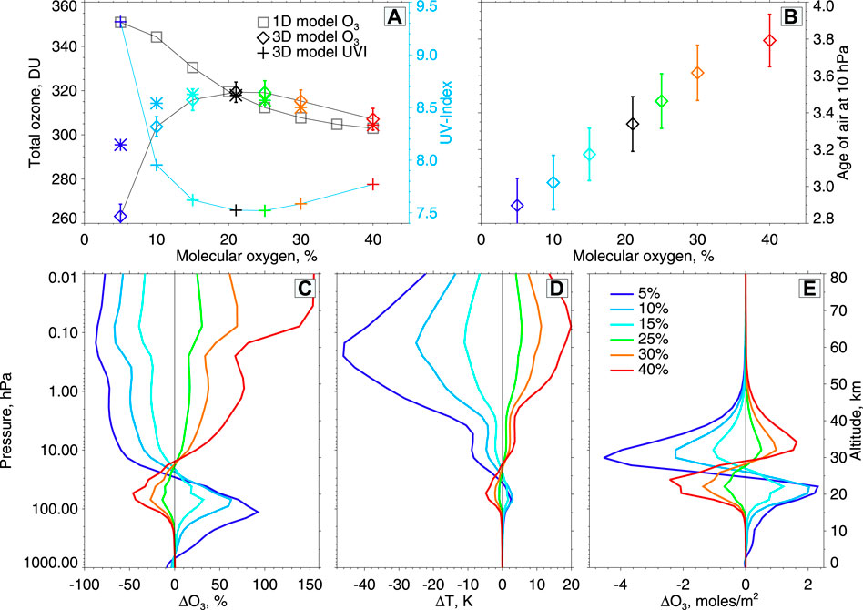
FIGURE 1. (A) Global mean total column O3 (in DU) for seven experiments differing by O2 levels (5%; 10%; 15%; 21%; 25%; 30%; 40%) obtained from a 1D model (grey squares) and 3D model (coloured diamonds) and the UV-index (UVI, coloured crosses with a black line) calculated from the 3D model O3 fields at local noon using an approximation from a previous study (Madronich, 2007). (B) Global mean age of air (in years) at 10 hPa for the seven experiments. (C) Difference between the sensitivity and the reference (O2 = 21%) experiments in the tropics (200S-200N) for O3 mixing ratio (in %) (D) Same difference for temperature (in K). (E) Same difference for O3 partial column (in molecules/m2). All results are averaged over the last 10 years of model integration. The error bars in panels a and b indicate 1σ uncertainty derived from the mean values for each of the 10 years.
To explain our results, we further highlight three mechanisms that dominate the global O3/O2 relationship in the considered 5%–40% O2 variation range: first, the “self-healing effect” of the ozone layer introducing a vertical dipole in the O3 response; second, an O2-dependent altitude and efficiency of maximum chemical O3 production via R2; and third, the subsequent changes in heating by O3 via R2 and R3 and, therefore, the speed of the Brewer-Dobson Circulation (BDC), which in turn determines O3 transport pathways (Dobson et al., 1929; Butchart, 2014) and distribution to mid- and high latitudes. These effects are separately discussed in detail below.
Although the total column O3 does not change dramatically with changing O2, the vertical O3 profile is strongly redistributed in the tropics, the main O3 production region (Figure 1E). This effect is known as “self-healing” and has been widely discussed in previous studies (Haigh and Pyle, 1982; Dutsch et al., 1991; Harfoot et al., 2007). For the low O2 cases, the lower levels of O3 in the upper parts of the stratosphere are compensated by the higher levels of O3 at lower altitudes, because lower O2 at high altitudes allows more O3-producing UV (<242 nm) to reach the lower layers. The situation is mirrored for the high O2 cases. The amplitude of this vertical redistribution is partly lowered by the reversed effects of the O3-destroying UV (>242 nm), so that the higher O3 production in the lower layers for the low O2 cases is also compensated by increased destruction through R3. These chemical-radiative effects of O2 on O3 can be well captured by both 1-D and 3-D models, but they do not explain the shape of the total O3 changes in Figure 1A, since the tropics still self-maintain a roughly constant amount of column-integrated O3.
The second important process influencing the O3/O2 relationships in the tropics is related to the air density’s impact on the effectiveness of O3 production, which we explain using Figures 1C, E. At present, the level of the most efficient O3 production is situated at an altitude of around 40 km (Seinfeld and Pandis, 2016). Manipulating atmospheric oxygen’s proportion moves the altitude of maximum O3 production up (in case of increased O2) or down (in case of decreased O2) (Ratner and Walker, 1972; Levine et al., 1979; Kasting and Donahue, 1980). In the case of a high O2 experiment (O2 = 40%) the level of production in the tropics goes up and then UV is absorbed at lower densities, which makes the process of O3 production less effective and results in the decrease in total O3 (Figure 1A). However, shifting the production region upwards does not affect R1; in all modeled cases, all photons with wavelengths shorter than 242 nm will be absorbed, and they will still produce the same amount of atomic oxygen in the total column. In contrast, R2 will be affected, because the higher the O2 photolysis region, the less “M” there is, so the larger the chance for O to get chemically paired up with other species (e.g., Cl or NO). Accordingly, in the low O2 case, it would be expected that more O3 would be produced, since the level of maximum production is shifted to lower altitudes, as it was presented by some previous studies based on 1-D models (Ratner and Walker, 1972; Levine et al., 1979; Kasting and Donahue, 1980). However, in our 3-D model case, the low O2 cases show less O3 in the total column in the O2 range where all ozone-producing photons are still fully absorbed in the atmosphere and not lost at the ground. This clearly differs from our 1-D results, as shown in Figure 1A, and undermines the explanation based on the air density’s influence. Therefore, the process responsible for the descending shape of the curve in Figure 1A for low O2 cases is most likely related to the third factor, namely, atmospheric transport.
The vertical dipole in O3 responses to atmospheric O2 changes has a direct impact on temperatures (Figure 1D). In the upper parts of the atmosphere, smaller O2 levels result in lower temperatures, and vice versa. Following the relative O3 changes in Figure 1C, the most pronounced temperature differences are found near the stratopause (1 hPa), with a warming of up to 20 K for the highest O2 case (red line) and a very strong cooling of around 45 K for the lowest O2 case (dark blue line). Around 20–30 hPa, there is a reversal of this pattern, but the temperature modulations in the lower stratosphere are less pronounced than those in the upper atmosphere. Temperature differences in the low-latitude stratosphere affect the global meridional circulation, overcompensating the air density’s effect and contributing to the shape of the curve in Figure 1A. The Brewer-Dobson circulation, induced by wave activity, introduces the meridional transport in the stratosphere (Plumb, 2002). Air is transported either through the deep branch, displacing tropical stratospheric air to the mid-latitudes and polar regions following the long route in the high stratosphere and mesosphere, or through the shallow branch, transporting air from the tropical lowermost stratosphere directly to mid-latitudes. To identify potential impacts of the temperature changes on stratospheric dynamics, we analyzed the simulated stratospheric mean age of air (AOA), implemented as an inert tracer with linearly increasing lower boundary conditions (“clock-tracer”) (Hall and Plumb, 1994). Figure 1B shows that the transport accelerates for the low O2 cases, which is proven by the relatively young AOA, and vice versa. This intensified transport out of the tropics seems to be the dominating process responsible for the inverted U-shaped curve in Figure 1A. An explanation of this nonlinear redistribution of O3 requires a closer inspection of regional differences in ozone and stratospheric dynamical changes, which is discussed further in Sections 3.2, 3.3, respectively.
Due to the “self-healing” effect explained earlier, the total O3 in the tropics is less sensitive to O2 changes than in high latitudes where larger differences are generally observed. This has been shown for the first time in the 2-D model study (Harfoot et al., 2007). In their study the tropics were less sensitive to O2 variations while high latitudes changes were more pronounced than in our simulations. For the 5% O2 case, however, there are still strong >40% changes even in the tropics, which is also seen in Figure 1E as a negative anomaly in the middle stratosphere being much larger than its lower counterpart. This could be related to either the ozone production profile being shifted to the troposphere, where the dynamical lifetime of ozone is shorter, or to the much faster BDC in the stratosphere that intensifies the transport of ozone from the tropics.
Both polar regions are significantly affected, however it is clear from Figure 2 that northern and southern high latitudes do not mirror each other but react differently to O2 changes. For example, the global mean total O3 for the 25% O2 case is identical to the reference case, however, the interhemispheric distribution differs: the 25% O2 case shows a decrease in the Northern Hemisphere (NH) and an increase in the Southern Hemisphere (SH). In contrast to the 2-D study (Harfoot et al., 2007), which observed a positive O3 change in high latitudes for the high O2 cases, all our experiments show negative O3 changes over northern high latitudes, with pronounced effects visible over Canada and Northern Europe even for the moderate O2 changes. The SH shows a different behavior, with high-latitude changes being negative for lower-than-present O2 levels, but positive for higher-than-present O2 experiments. Such interhemispheric asymmetry has also been shown by another 3-D study by Ji et al. (2023) using the WACCM6 model. These geographical redistributions can be predominantly explained by transport processes, which are particularly important in regions where the chemical lifetime is larger than dynamical timescales, i.e., in the lower stratosphere, where chemical species live long enough to be transported before being destroyed by catalytic cycles or photolysis (Dessler, 2000). Polar regions have very little O3 production in situ, therefore the amount of O3 highly depends on the transport from the tropics. The air transported through the deep and shallow branches of the BDC can mix on the way to the poles. However, whether this air gets to the poles or stays in the surf-zone depends on the strength of the polar vortex, which constitutes a transport barrier. If the vortex is strong and isolated, little mixing occurs between older air transported by the deep branch and younger air transported by the shallow branch, which is the case for the SH. However, in the NH, the polar vortex tends to be weaker due to the surface heterogeneity characterized by more pronounced waves, breaking the transport barrier of the vortex (Strahan et al., 2015). Such asymmetry between the strength of the polar vortices, making the NH more affected by the mixing with mid-latitudes and the SH more affected by the deep branch of the BDC in our model, is one of the dynamical effects, which explains some redistributions presented in Figure 2. To better understand such transport effects, it is necessary to closely analyze the vertical cross-sections of stratospheric changes, which is performed in the next section.
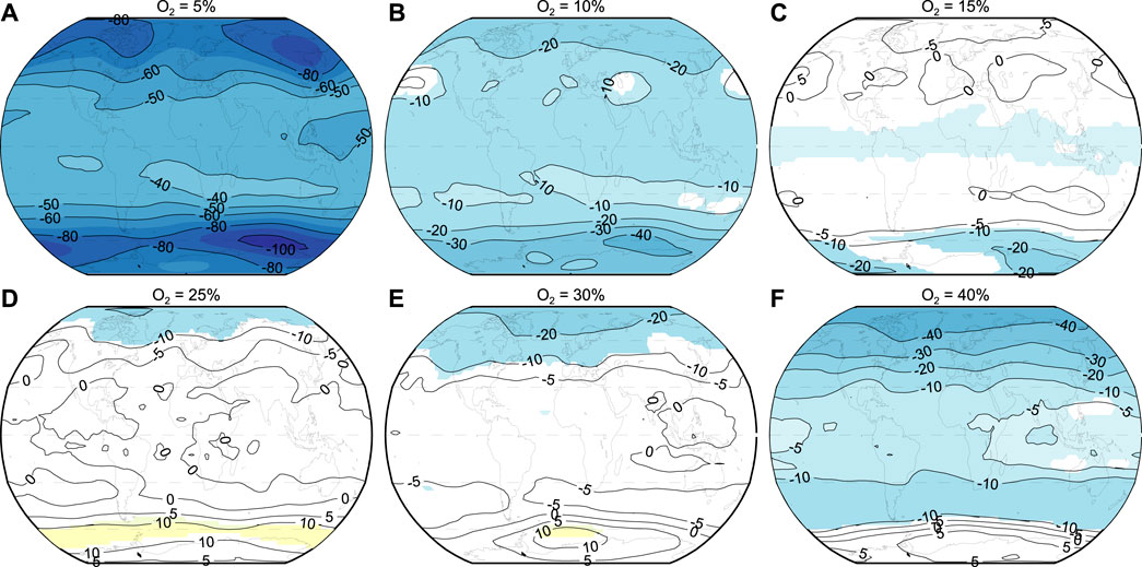
FIGURE 2. Total ozone column differences (in Dobson units) relative to the reference (O2 = 21%) experiment averaged over the last 10 years of integration. Each of the maps corresponds to the individual experiments with different molecular oxygen levels, specified above each panel (A–F). Horizontal dashed lines mark the −60, −30, 0, 30, and 60 deg latitudes. White areas indicate non-significance (at the 95% statistical significance level according to the Student t-test).
To understand varying responses of NH and SH to modeled O2 cases, the vertical cross-sections explaining the O3 transport pathways need to be discussed. Figures 3, 4 show seasonal mean changes in O3, temperature and zonal wind for the 10% and 40% O2 cases compared to the reference case for winter in the NH (DJF) (Figure 3) and in the SH (JJA) (Figure 4). To better understand the differences between the hemispheres, we discuss additional effects, which are based on the interaction and interdependency of O3, stratospheric transport, temperature and winds. All being linked to each other and coupled with previously discussed effects.
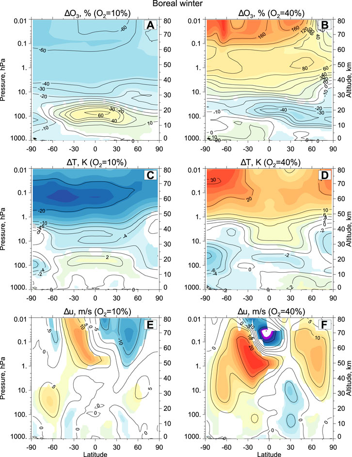
FIGURE 3. Zonal mean differences relative to the reference experiment (O2=21%) of: O3 volume mixing ratio [%] (A,B), temperature [K] (C,D), and zonal winds [m/s] (E,F). All averaged over the last 10 years of integration for boreal winter (December, January, February (DJF)). White areas indicate non-significance (at the 95% statistical significance level according to Student’s t-test). Panels a, c, e refer to our 10% O2 experiment, whereas b, d, f to our 40% O2 experiment. Coloured contours are discretized every 10% (for O3 volume mixing ratio in the panels a and b), every 2K (for temperature in the panels c and d), and every 5 m/s (for winds in the panels e and f). 10% was chosen as the low case, because it has a similar amplitude to 40% (judging from Figure 2C) and because it was the lowest O2 concentration over Phanerozoic Eon.
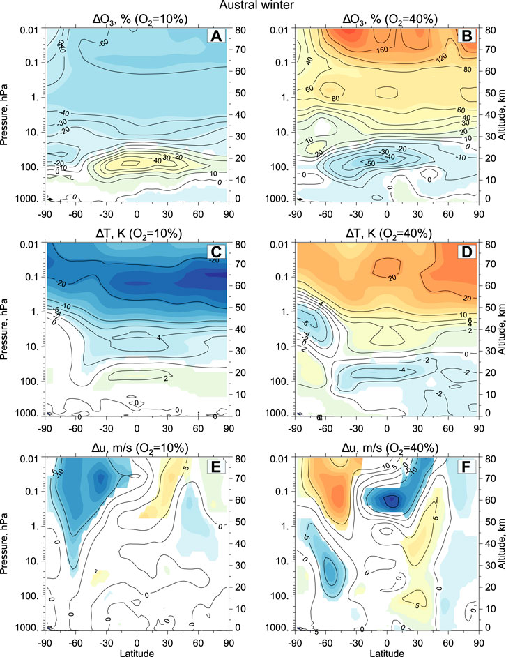
FIGURE 4. Same as Figure 3, but for austral winter [June, July, August (JJA)].
Figure 1B presents a deceleration of the BDC for the high O2 case, manifested through the older AOA, which implies a strongly isolated vortex. Conversely, for the low O2 case an intensification of the meridional circulation is observed, resulting in younger air, and the vortices become weaker which allows enhanced mixing. AOA changes range between around −10% and +10% for the low and high O2 cases, respectively. The change occurs all over the stratosphere but is more pronounced in its middle and lower parts. Zonal wind changes as shown in Figures 3E, F are consistent with these results. Looking at the 40% O2 case in Figure 3B, it can be seen that the low O3 anomaly propagates from the tropics to the mid-latitudes and further to the poles, due to the deceleration of the BDC. In that case, the shallow branch dominates, and the contribution of the high O3 subsidence in the mid-latitudes and in the vortex is largely decreased. In contrast, there is a clear dynamical non-linearity between high and low O2 cases. Looking at the 10% O2 case in Figure 3A, it is evident that the positive anomaly of the lower tropical stratosphere cannot propagate into middle and high latitudes as much as in the high O2 case. This can be explained by the decreased strength of the vortex (Figure 3E) and accelerated BDC. In that case, the shallow branch would still transport some part (about 20%–30%) of the anomaly to mid-latitudes, but there would be a much more pronounced effect of the negative anomaly, subsiding from above in the mid-latitudes and over the pole. Dynamics modify the importance of mixing in the middle stratosphere, which is clearly visible by the difference between the isolines of the O3 changes. Skewness of the isotherms in the lower-middle stratosphere suggests that the meridional temperature gradient is altered, which induces acceleration (40% O2 case) or deceleration (10% O2 case) of the polar vortices, based on the thermal wind formulation. This is also reflected in the panels a and b of Figures 3, 4, presenting O3 mixing ratio. The isolines for O3 anomalies in the middle stratosphere are much smoother (more horizontally linear) for the low O2 experiment, presenting the weak vortex and domination of subsidence, and much more skewed for the high O2 case, so the high latitudes are dominated by the lower part of the dipole.
In the SH, the same processes are operating, but the difference occurs due to the fact that the southern polar vortex is two times stronger in comparison to the northern one (Harvey et al., 2002). Looking at Figure 4, it is evident that the dynamical effect of the SH is different, which was also visible on the maps in Figure 2. For the 10% O2 case, the BDC accelerates, hence the AOA becomes younger. There occurs also a weakening of the polar vortex and a clear competition between the transport by the shallow branch and subsidence by the deep branch, with a pronounced domination of the latter one. This is also supported by the horizontally straight isolines of O3 in the middle stratosphere, which suggest the enhanced effect of the air coming from above. In contrast, looking at the 40% O2 case, it can be observed that the BDC is decelerated and there is a decrease of subsidence and clear domination of the negative anomaly coming through the shallow branch and mixing into the pole. In that case the polar vortex is generally stronger, however its strength in Figure 4 is not so pronounced and uniform, possibly due to the prescribed quasi-biennial oscillation in the model. It is worth noting that the acceleration of the BDC in the 10% O2 case indeed results in less O3 staying in the source region due to the fast transport, however for the same reason it also results in less O3 being destroyed. Conversely, in the 40% O2 case, a slower BDC can contribute to more O3 being destroyed, since there is more time for the destruction processes to take place.
To confirm further our conclusions about the interdependence of ozone, temperature, and transport, in Figure 5 we present the anomalies of the age of air, like other variables in Figures 3, 4, but annual mean. The Figure shows intensification of the transport related to deep branch of the BDC under the 10% experiment and the opposite under the 40% experiment, represented as AOA change of up-to ± half a year in the middle and the upper stratosphere. Both cases also illustrate that the transport change related to the shallow branch has an opposite sign, which is reflected as very low and statistically insignificant values in the lower and the lowermost stratosphere, indicating the competition between the transport changes through the shallow and deep branches.
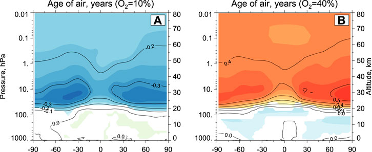
FIGURE 5. Annual and zonal mean differences of the age of air (years) in two oxygen experiments (O2=10% in (A) and O2=40% in (B)) relative to the reference experiment (O2=21%). Both are averaged over the last 10 years of integration. White areas indicate non-significance (at the 95% statistical significance level according to Student’s t-test).
Our analysis indicates that large low latitude changes in O3 alter the temperature regime of the stratosphere, inducing additional changes to dynamics and O3 transport that explains the non-linearity in the total O3 response at mid and high latitudes. Although this mechanism explains the majority of the observed signal, there are many additional feedback loops involved, which contribute to the overall picture. The strengthening and isolation of the vortex due to the temperature gradient would further contribute to the colder temperatures over the pole, affecting the formation of polar stratospheric clouds and related heterogeneous chemistry (Prather, 1992) and denitrification processes. Moreover, changes of temperature in other stratospheric regions would also influence the chemical reaction rates, while the change of available UV and oxidants at different heights would influence CH4 and N2O oxidation rates, both of which will modulate the speed of the O3 destruction by catalytic cycles. Temperature variations at the tropical tropopause might also affect the stratospheric water vapor content. A separate analysis reveals that H2O influx from the troposphere would increase by 30% in the low O2 case (10%) and decrease by 30% for the high O2 case (40%). This could contribute to the results of our study as water vapor provides a source for hydroxyl catalytic cycles, which dominate the O3 destruction above the stratopause (Stenke and Grewe, 2005).
To test the sensitivity of our findings to the underlying atmospheric state and potential biases in the model dynamics representation, we have rerun our experiments using another SOCOL model version, SOCOL-MPIOM (Muthers et al., 2014). This model employs an interactive ocean and has quite different behavior in terms of polar vortex biases and ozone-dynamics feedback compared to SOCOL-AERv2 (Friedel et al., 2023). In addition, it was used under the pre-industrial setup (year 1850) meaning lower greenhouse gas and ozone precursor levels and no anthropogenic halogens in the atmosphere. Comparison of the O3 column dependence on the O2 levels under two model setups is presented in Figure 6 for different latitude bands. SOCOL-MPIOM simulations mostly show the ozone column maximization around 15%–21% of O2, compared to the 21%–25% in the SOCOL-AERv2 case, with the largest differences appearing in the polar regions. Nevertheless, both modeling setups qualitatively still agree on the shape of the O3 dependence on O2, namely, increasing O3 column for lower than near-present O2 levels and decreasing O3 column for the higher than near-present O2 levels, as well as the higher amplitude of changes in the polar regions. This analysis illustrates that indeed some of the features discussed in the previous sections could be potentially affected by the model differences in the climatology of the stratospheric dynamics and composition, especially for small variations around the near-present level. However, the ozone-temperature-transport feedback would still act as an underlying modulating mechanism, favoring negative ozone column anomalies in the middle and higher latitudes even for the higher-than-present O2 levels.
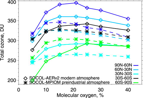
FIGURE 6. Total column O3 (in DU) for seven experiments differing by O2 levels (5%; 10%; 15%; 21%; 25%; 30%; 40%) obtained from a SOCOL-AERv2 model with modern atmospheric setting (solid line with a diamond sign) and from a SOCOL-MPIOM model with pre-industrial atmospheric conditions (dashed line with an asterisk sign). Different latitudinal bands are marked by colors.
It is important to note that the highlighted mechanism could act differently in the much lower pre-Phanerozoic O2 levels, as more ozone-producing UV will reach the troposphere. In addition, several studies have reported substantial climate effects due to O2 variations impacts on atmospheric pressure, such as global surface temperatures, water vapor concentrations, precipitation, and the hydrological cycle (Poulsen et al., 2015; Wade et al., 2019; Edkins and Davies, 2021). Such changes would impact the tropopause height and shape, tropospheric wave forcing, and states of the polar and subtropical jets, introducing additional modulation to the discussed stratospheric processes, which is not considered in our study as well as in other previous chemistry-focused studies. Thus, more research is needed to combine both factors and to test transport processes’ importance in other models under Phanerozoic and pre-Phanerozoic O2 variations.
Our findings show that total O3 peaks around the near-present O2 levels and alterations in the atmospheric O2 result in less total O3 being sustained globally. The study shows that a variety of complex processes influences the O3/O2 relationship. In the considered 5%–40% O2 range, the O3 changes for high and low O2 cases can be to a large extent explained by the combination of three processes, all interdependent and linked to each other: dynamical changes resulting from the acceleration/deceleration of the BDC, “self-healing” effect, and the air density’s influence on the O3 production in the total column. While the “self-healing” and air density effects dominate in the tropics, the changes in the dynamics are responsible for the more pronounced changes in the high latitudes. “Self-healing” introduces the vertical dipole in the low-latitude O3 and temperature changes and therefore modifies the dynamics, which always work in favor of the negative part of the tropical O3 anomaly that is effectively transported to the mid- and high-latitudes. These processes are summarized in Figure 7. Moreover, there exists an interhemispheric asymmetry, which is explained by the effect of enhanced mixing of the lowermost stratosphere in the NH and the dominating role of large-scale advective transport in the SH, which, however, could be different under different past geographical positioning of continents.
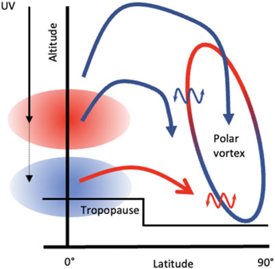
FIGURE 7. Schematic summary of the processes in the winter hemisphere illustrating the results of the study for the higher-than-present O2 levels. Black vertical lateral line represents the change in the UV incident flux, because of the ozone mixing ratio changes in the tropics, represented as reddish and bluish oval areas corresponding to the positive and negative ozone anomalies respectively due to the oxygen change. These variations cause the local temperature changes of the same sign, which further influences the speed of the polar vortex and triggers the change in the speed of the BDC, represented as blue lines for deceleration of the deep branch and red line for some acceleration of the shallow branch. The speed of the polar vortex modulates the mixing of the mid-latitude regions with the polar regions, represented by wavy arrows. For the lower-than-present O2 levels, colors would be inverted.
Our results are contrary to previous 1-D or 2-D studies covering the Phanerozoic Eon range, which either showed a positive monotonic correlation of global annual mean O3 and atmospheric O2 (Harfoot et al., 2007), reported an O3 decrease with atmospheric O2 (Ratner and Walker, 1972), or discovered a peak in O3 column around 0.5 of the present atmospheric level (Kasting et al., 1985), however have similarities with the recent 3-D modeling papers (Way et al., 2017; Ji et al., 2023). We argue that changes in the composition can affect the dynamics, e.g., via O3-induced changes in the BDC. Meridional ozone redistribution due to O2 changes has been shown for the first time in the 2D model study (Harfoot et al., 2007), however in their model it was predominantly defined by the transport of O3 by the deep branch of the BDC (middle and higher stratosphere) without any competing effects in the lower stratosphere and no interhemispheric asymmetries. This could be related to the simplifications of the 2-D transport and wave drag schemes. Three other recent studies (Way et al., 2017; Cooke et al., 2022; Ji et al., 2023) also exploited 3-D chemistry-climate models like in our case, however the main focuses of these studies have been different to ours and the linearity of the O3/O2 relationship has only briefly been touched. One of these studies showed a continuously linear O3/O2 relationship up to the present atmospheric level and to the one experiment that they performed with higher-than-present O2 (31.5%) (Cooke et al., 2022), whereas the other one showed a clear saturation of the O3/O2 relationship around the present level (Way et al., 2017), which is consistent with us, however with no experiments beyond that. Unfortunately, both studies did not present and discuss the details of their ozone and temperature changes in the stratosphere, which complicated the identification of potential reasons for this disagreement. Finally, our results generally agree with the latest paper by Ji et al. (2023), which further analyzed the Cooke et al. (2022) simulations and showed non-linearities in the high-latitude ozone column response and highlighted the potential importance of transport processes.
It should be emphasized that the intention of our model study is not to present new estimates of atmospheric O3 concentrations during the Phanerozoic Eon, but to investigate the details of the O3 response to atmospheric O2 concentration changes taking dynamical feedback effect into account. Therefore, our model’s set-up contains simplifications, such as the lack of an interactive ocean for the main model setup, as well as fixed air density, present-day composition (ODS, O3 precursors) and orography, explained in the methods section. However, under the realistic transient setup we would expect a stronger or weaker sensitivity of the system to the O2 changes, but not a qualitatively different result. This is because, for whatever climatic background, the O2 change would always result in a tropical O3 and temperature vertical dipole, which is known from the Chapman cycle and basic radiative transfer (Brassuer and Solomon, 2005). And similarly, the large temperature changes in the sun-lit stratosphere would also have to induce the rearrangement of the stratospheric circulation, despite the climatic setting used. In a realistic transient setup, there would indeed be many other strong and important factors, but the dynamics would still be acting behind as a modulator. This has been tested using another model as explained in the methods and in the last section of the results concerning sensitivity analysis. Therefore, our paper brings useful insights for other studies focusing on the long-term O3/O2 relationship, namely, the importance of the chemistry radiative transport feedback that can strongly shape the regional and global O3 response to the O2 changes.
The datasets presented in this study can be found in online repositories. The names of the repository/repositories and accession number(s) can be found below: https://doi.org/10.5281/zenodo.5733121.
IJ drafted most of the paper, analyzed the data, and visualized some of the results. TS supervised IJ, assisted in data analysis, and visualized the final results. TE and ER designed model experiments and performed main simulations. JS performed simulations with the SOCOL-MPIOM model. TP, HR, AS, and GC contributed with their expertise in atmospheric chemistry and dynamics and drafted parts of the text. All authors contributed to the article and approved the submitted version.
This research has been supported by the Schweizerischer Nationalfonds zur Förderung der Wissenschaftlichen Forschung (project POLE, Polar Ozone Layer Evolution; grant no. 200020- 182239) and by the Karbacher Fonds, Graubünden, Switzerland. GC also acknowledges funding from the Schweizerischer Nationalfonds zur Förderung der Wissenschaftlichen Forschung (Ambizione Grant N. PZ00P2_180043). The work was partially carried out at the St. Petersburg State University “Ozone Layer and Upper Atmosphere Research laboratory” with the support of the Government of the Russian Federation (grant no. 075-15-2021-583).
Model simulations have been performed on the ETH Zürich cluster EULER.
The authors declare that the research was conducted in the absence of any commercial or financial relationships that could be construed as a potential conflict of interest.
All claims expressed in this article are solely those of the authors and do not necessarily represent those of their affiliated organizations, or those of the publisher, the editors and the reviewers. Any product that may be evaluated in this article, or claim that may be made by its manufacturer, is not guaranteed or endorsed by the publisher.
Adiatma, Y. D., Saltzman, M. R., Young, S. A., Griffith, E. M., Kozik, N. P., Edwards, C. T., et al. (2019). Did early land plants produce a stepwise change in atmospheric oxygen during the Late Ordovician (Sandbian ∼458 Ma)? Palaeogeogr. Palaeoclimatol. Palaeoecol. 534, 109341. doi:10.1016/j.palaeo.2019.109341
Berkner, L. V., and Marshall, L. C. (1965). On the origin and rise of oxygen concentration in the Earth’s atmosphere. J. Atmos. Sci. 22, 225–261. doi:10.1175/1520-0469(1965)022<0225:otoaro>2.0.co;2
Berner, R. A., Beerling, D. J., Dudley, R., Robinson, J. M., and Wildman, R. A. (2003). Phanerozoic atmospheric oxygen. Annu. Rev. Earth Planet. Sci. 31, 105–134. doi:10.1146/annurev.earth.31.100901.141329
Brasseur, G. P., and Solomon, S. (2005). Aeronomy of the middle atmosphere. 3rd edn. Germany: Springer.
Butchart, N. (2014). The Brewer-Dobson circulation. Rev. Geophys. 52, 157–184. doi:10.1002/2013rg000448
Catling, D. C., and Kasting, J. F. (2017). Atmospheric evolution on inhabited and lifeless worlds. Cambridge: Cambridge University Press.
Cooke, G. J., Marsh, D. R., Walsh, C., Rugheimer, S., and Villanueva, G. L. (2022). Variability due to climate and chemistry in observations of oxygenated Earth-analogue exoplanets. Mon. Notices R. Astronomical Soc. 518 (1), 206–219. doi:10.1093/mnras/stac2604
Dessler, A. E. (2000). The chemistry and Physics of stratospheric ozone. San Diego, CA: Academic Press.
Dobson, G. M. B., Harrison, D. N., and Lawrence, J. (1929). Measurements of the amount of ozone in the Earth’s atmosphere and its relationto other geophysical conditions. Proc. R. Soc. A122, 456–486.
Dutsch, H. U., Bader, J., and Staeheli, J. (1991). Separation of solar effects on ozone from anthropogenically produced trends. J. Geomag. Geoelectr. 4, 657–665. doi:10.5636/jgg.43.supplement2_657
Duursma, E. K., and Boission, M. P. R. M. (1994). Global oceanic and atmospheric oxygen stability considered in relation to the carbon cycle and to different time scales. Oceanol. Acta 17, 117–141.
Edkins, N. J., and Davies, R. (2021). Atmospheric pressure and snowball Earth deglaciation. J. Geophys. Res. Atmos. 126 (24). doi:10.1029/2021jd035423
Egorova, T. A., Karol, I. L., and Rozanov, E. V. (1997). The influence of ozone content loss in the lower stratosphere on the radiative balance of the troposphere, Physics of atmosphere and ocean. Russ. Acad. Sci. 33 (N4), 492–499.
Egorova, T., Rozanov, E., Zubov, V., and Karol, I. (2003). Model for investigating ozone trends (MEZON). Izv. Atmos. Ocean. Phy. 39, 277–292.
Feinberg, A., Sukhodolov, T., Luo, B. P., Rozanov, E., Winkel, L. H. E., Peter, T., et al. (2019). Improved tropospheric and stratospheric sulfur cycle in the aerosol-chemistry-climate model SOCOL-AERv2. Geosci. Model Dev. 12, 3863–3887. doi:10.5194/gmd-12-3863-2019
Friedel, M., Chiodo, G., Sukhodolov, T., Keeble, J., Peter, T., Seeber, S., et al. (2023). Weakening of springtime Arctic ozone depletion with climate change. EGUsphere [preprint]. doi:10.5194/egusphere-2023-565
Haigh, J. D., and Pyle, J. A. (1982). Ozone perturbation experiments in a two-dimensional circulation model. Q.J R. Mater. Soc. 108, 551–574. doi:10.1002/qj.49710845705
Hall, T. M., and Plumb, R. A. (1994). Age as a diagnostic of stratospheric transport. J. Geophys. Res. 99, 1059. doi:10.1029/93jd03192
Harfoot, M. B. J., Beerling, D. J., Lomax, B. H., and Pyle, J. A. (2007). A two-dimensional atmospheric chemistry modeling investigation of Earth’s Phanerozoic O3 and near-surface ultraviolet radiation history. J. Geophys. Res. 112, D07308. doi:10.1029/2006jd007372
Harvey, V. L., Pierce, R. B., Fairlie, T. D., and Hitchman, M. H. (2002). A climatology of stratospheric polar vortices and anticyclones. J. Geophys. Res. 107 (D20), 4442. doi:10.1029/2001jd001471
Herndon, J., Hoisington, R., and Whiteside, M. (2018). Deadly ultraviolet UV-C and UV-B penetration to Earth’s surface: human and environmental health implications. JGEESI 14, 1–11. doi:10.9734/jgeesi/2018/40245
Ji, A., Kasting, J. F., Cooke, G. J., Marsh, D. R., and Tsigaridis, K. (2023). Comparison between ozone column depths and methane lifetimes computed by one- and three-dimensional models at different atmospheric O2 levels. R. Soc. Open Sci. 10, 230056. doi:10.1098/rsos.230056
Kasting, J. F., and Donahue, T. M. (1980). The evolution of atmospheric ozone. J. Geophys. Res. 85, 3255. doi:10.1029/jc085ic06p03255
Kasting, J. F., Holland, H. D., and Pinto, J. P. (1985). Oxidant abundances in rainwater and the evolution of atmospheric oxygen. J. Geophys. Res. 90, 10497–10510. doi:10.1029/jd090id06p10497
Kozakis, T., Mendonça, J. M., and Buchhave, L. A. (2022). Is ozone a reliable proxy for molecular oxygen? A&A 665, A156. doi:10.1051/0004-6361/202244164
Large, R. R., Mukherjee, I., Gregory, D., Steadman, J., Corkrey, R., and Danyushevsky, L. V. (2019). Atmosphere oxygen cycling through the proterozoic and phanerozoic. Min. Deposita 54, 485–506. doi:10.1007/s00126-019-00873-9
Leaf, A. (1993). “Loss of stratospheric ozone and health effects of increased ultraviolet radiation,” in Critical condition: Human health and environment. Editors E. Chivian, M. McCally, H. Hu, and A. Haines (Cambridge, MA: The MIT Press), 139–150.
Lefohn, A. S., Malley, C. S., Smith, L., Wells, B., Hazucha, M., Simon, H., et al. (2018). Tropospheric ozone assessment report: global ozone metrics for climate change, human health, and crop/ecosystem research. Elem. Sci. Anthropocene 1 January 6, 6 27. doi:10.1525/elementa.279
Lenton, T. M., Dahl, T. W., Daines, S. J., Mills, B. J. W., Ozaki, K., Saltzman, M. R., et al. (2016). Earliest land plants created modern levels of atmospheric oxygen. Proc. Natl. Acad. Sci. U. S. A. 113, 9704–9709. doi:10.1073/pnas.1604787113
Levine, J. S., Hays, P. B., and Walker, J. C. G. (1979). The evolution and variability of atmospheric ozone over geological time. Icarus 39, 295–309. doi:10.1016/0019-1035(79)90172-6
Lyons, T. W., Reinhard, C. T., and Planavsky, N. J. (2014). The rise of oxygen in Earth’s early ocean and atmosphere. Nature 506, 307–315. doi:10.1038/nature13068
Madronich, S. (2007). Analytic formula for the clear-sky UV index. Photochem. Photobiol. 83, 1537–1538. doi:10.1111/j.1751-1097.2007.00200.x
Marshall, J. E. A., Lakin, J., Troth, I., and Wallace-Johnson, S. M. (2020). UV-B radiation was the Devonian-Carboniferous boundary terrestrial extinction kill mechanism. Sci. Adv. 6, eaba0768. doi:10.1126/sciadv.aba0768
Meinshausen, M., Smith, S., Calvin, K., Daniel, J., Kainuma, M., Lamarque, J.-F., et al. (2011). The RCP greenhouse gas concentrations and their extensions from 1765 to 2300. Clim. Change 109, 213–241. doi:10.1007/s10584-011-0156-z
Muthers, S., Anet, J. G., Stenke, A., Raible, C. C., Rozanov, E., Brönnimann, S., et al. (2014). The coupled atmosphere–chemistry–ocean model SOCOL-MPIOM. Geosci. Model Dev. 7, 2157–2179. doi:10.5194/gmd-7-2157-2014
Nowack, P., Luke Abraham, N., Maycock, A., Braesicke, P., Gregory, J. M., Joshi, M. M., et al. (2015). A large ozone-circulation feedback and its implications for global warming assessments. Nat. Clim. Change 5, 41–45. doi:10.1038/nclimate2451
Oehrlein, J., Chiodo, G., and Polvani, L. M. (2020). The effect of interactive ozone chemistry on weak and strong stratospheric polar vortex events. Atmos. Chem. Phys. 20, 10531–10544. doi:10.5194/acp-20-10531-2020
Plumb, R. A. (2002). Stratospheric transport. J. Meteorological Soc. Jpn. Ser. II 80, 793–809. doi:10.2151/jmsj.80.793
Poulsen, C. J., Tabor, C., and White, J. D. (2015). Long-term climate forcing by atmospheric oxygen concentrations. Science 348, 1238–1241. doi:10.1126/science.1260670
Prather, M. J. (1992). More rapid polar ozone depletion through the reaction of HOCI with HCI on polar stratospheric clouds. Nature 355, 534–537. doi:10.1038/355534a0
Ratner, M. I., and Walker, J. C. G. (1972). Atmospheric ozone and the history of life. J. Atmos. Sci. 29, 803–808. doi:10.1175/1520-0469(1972)029<0803:aoatho>2.0.co;2
Roeckner, E., Bäuml, G., Bonaventura, L., Brokopf, R., Esch, M., Giorgetta, M., et al. (2003). The atmospheric general circulation model ECHAM 5. PART I: model description. Rep./Max-Planck-Institut für Meteorol. 349.
Seinfeld, J. H., and Pandis, S. N. (2016). Atmospheric chemistry and Physics: From air pollution to climate change. Hoboken: John Wiley & Sons.
Sheng, J. X., Weisenstein, D. K., Luo, B. P., Rozanov, E., Stenke, A., Anet, J., et al. (2015). Global atmospheric sulfur budget under volcanically quiescent conditions: aerosol-chemistry-climate model predictions and validation. J. Geophys. Res. Atmos. 120, 256–276. doi:10.1002/2014jd021985
Stenke, A., and Grewe, V. (2005). Simulation of stratospheric water vapor trends: impact on stratospheric ozone chemistry. Atmos. Chem. Phys. 5, 1257–1272. doi:10.5194/acp-5-1257-2005
Stenke, A., Schraner, M., Rozanov, E., Egorova, T., Luo, B., and Peter, T. (2013). The SOCOL version 3.0 chemistry–climate model: description, evaluation, and implications from an ad-vanced transport algorithm. Geosci. Model Dev. 6, 1407–1427. doi:10.5194/gmd-6-1407-2013
Strahan, S. E., Oman, L. D., Douglass, A. R., and Coy, L. (2015). Modulation of Antarctic vortex composition by the quasi-biennial oscillation. Geophys. Res. Lett. 42 (10), 4216–4223. doi:10.1002/2015gl063759
Wade, D. C., Abraham, N. L., Farnsworth, A., Valdes, P. J., Bragg, F., and Archibald, A. T. (2019). Simulating the climate response to atmospheric oxygen variability in the phanerozoic: A focus on the Holocene, cretaceous and permian. Clim. Past 15 (4), 1463–1483. doi:10.5194/cp-15-1463-2019
Way, M. J., Aleinov, I., Amundsen, D. S., Chandler, M., Clune, T., Del Genio, A. D., et al. (2017). Resolving orbital and climate keys of Earth and extraterrestrial environments with dynamics (ROCKE-3D) 1.0: A general circulation model for simulating the climates of rocky planets. ApJS 231, 12. doi:10.3847/1538-4365/aa7a06
Keywords: stratospheric dynamics, ozone layer, O3/O2 relationship, chemistry-dynamics feedback, Phanerozoic Eon
Citation: Józefiak I, Sukhodolov T, Egorova T, Chiodo G, Peter T, Rieder H, Sedlacek J, Stenke A and Rozanov E (2023) Stratospheric dynamics modulates ozone layer response to molecular oxygen variations. Front. Earth Sci. 11:1239325. doi: 10.3389/feart.2023.1239325
Received: 13 June 2023; Accepted: 24 August 2023;
Published: 15 September 2023.
Edited by:
Jian Rao, Nanjing University of Information Science and Technology, ChinaReviewed by:
Qian Lu, China Meteorological Administration, ChinaCopyright © 2023 Józefiak, Sukhodolov, Egorova, Chiodo, Peter, Rieder, Sedlacek, Stenke and Rozanov. This is an open-access article distributed under the terms of the Creative Commons Attribution License (CC BY). The use, distribution or reproduction in other forums is permitted, provided the original author(s) and the copyright owner(s) are credited and that the original publication in this journal is cited, in accordance with accepted academic practice. No use, distribution or reproduction is permitted which does not comply with these terms.
*Correspondence: Iga Józefiak, aWdhLmpvemVmaWFrQGdtYWlsLmNvbQ==; Timofei Sukhodolov, VGltb2ZlaS5TdWtob2RvbG92QHBtb2R3cmMuY2g=
Disclaimer: All claims expressed in this article are solely those of the authors and do not necessarily represent those of their affiliated organizations, or those of the publisher, the editors and the reviewers. Any product that may be evaluated in this article or claim that may be made by its manufacturer is not guaranteed or endorsed by the publisher.
Research integrity at Frontiers
Learn more about the work of our research integrity team to safeguard the quality of each article we publish.