 Xiuying Wang
 Wanli Cheng
 Xueqing Zhang3
 Dehe Yang
 Song Xu
94% of researchers rate our articles as excellent or good
Learn more about the work of our research integrity team to safeguard the quality of each article we publish.
Find out more
ORIGINAL RESEARCH article
Front. Earth Sci., 27 December 2023
Sec. Atmospheric Science
Volume 11 - 2023 | https://doi.org/10.3389/feart.2023.1238541
The post-midnight irregularities in equator and its adjcent regions, which have remained least explored so far, are investigated using the in situ electron density (Ne) measurements from 2019 to 2021 obtained by the China Seismo-Electromagnetic Satellite (CSES) in the topside ionosphere. The followings are salient points of our findings: 1) Equatorial and low latitude post-midnight irregularities are distributed along the dip equator, exhibiting a wavenumber 4 longitude variation pattern and a seasonal variation pattern characterized by peaks in summer and winter and valleys in spring and autumn during low solar activity (LSA) period in the topside ionosphere, 2) The longitude variation pattern of post-midnight irregularities aligns with that of the background Ne, with irregularities concentrated at the peaks of background Ne, 3) The occurrence rate of post-midnight irregularities increases significantly with higher solar flux, which can be attributed to the rapid increase in the background Ne under LSA conditions. Additionally, the growth rate of occurrence rate varies across different longitudes, with the Pacific and the Atlantic longitudes standing out as prominent regions, and 4) Post-midnight irregularities in the topside ionosphere may have two possible origins. One is irregularities generated at the lower altitudes that drift upward into the topside ionosphere, while the other is the irregularities generated directly in the topside ionosphere. The latter is supported by the presence of conditions conducive to irregularity generation in the topside ionosphere during midnight hours in LSA period. Given the scarcity of research on post-midnight irregularity compared to post-sunset irregularity, further investigations are essential to fully comprehend their generation mechanisms. The abundance of post-midnight Ne measurements from the CSES satellite offers a valuable opportunity for this research, which can enhance our understanding of post-midnight ionospheric dynamics, and their variations with solar activity.
Ionospheric scintillations are fluctuations of radio wave signals caused by the scattering of irregularities in the ionosphere when radio waves traverse the ionosphere (Aarons, 1982; Kil and Heelis, 1998; Huang et al., 2001; Basu et al., 2002). Severe scintillation can prevent a GPS receiver from locking on to the signal and less severe scintillations can reduce the accuracy and the confidence of positioning results (Whalen, 1997; Kintner et al., 2007; Tsai et al., 2017). In addition, ionospheric scintillation can significantly degrade both the performance and availability of space-based communication and navigation systems (Groves et al., 1997; Basu et al., 2002; Gentile et al., 2006; Kintner et al., 2007). For these reasons, ionospheric scintillation has long been one of the focuses on ionosphere research. Equatorial scintillation is caused by the equatorial spread F (ESF) observed by ground-based ionosonde, and more appropriate name for ESF is Equatorial F-Region Irregularities or Equatorial F-Region Field Aligned Irregularities (FAIs) (Fejer and Kelley, 1980; Woodman, 2009); it is also called plasma depletion or plasma bubble (Burke, 1979; Singh et al., 1997; Kil and Heelis, 1998; Burke et al., 2004; Gentile et al., 2006). The naming convention will be followed in this paper, and all the above mentioned terms indicate the same phenomenon unless otherwise specified.
Though ionospheric scintillation has been studied extensively so far, it remains a difficult phenomenon to predict due to its complex variation with local time, season, geomagnetic activity, and solar cycle (Aarons, 1982; 1993; Whalen, 1997; Huang et al., 2002; Burke et al., 2004; Hei et al., 2005; Gentile et al., 2006; Su et al., 2006; Su et al., 2008; Tsai et al., 2017; Beshir et al., 2020; Jin et al., 2020; Wang et al., 2022). Previous studies show that ionospheric scintillations are mainly concentrated at three regions: the geomagnetic equator, the auroral ovals, and inside the polar caps (Aarons, 1982; Basu et al., 1988; Basu et al., 2002; Tsunoda, 1988; Jin et al., 2020). As scintillation is so severe in the Equator and its vicinity, it is the region most vulnerable to scintillation-induced communication problems. Therefore, many studies on scintillation have focused on this region (Abdu et al., 1985; Aarons, 1993; Kil and Heelis, 1998; Huang et al., 2001; Huang et al., 2002; Burke et al., 2004; Gentile et al., 2006; Heelis et al., 2010; Dao et al., 2011; Ajith et al., 2016; Jin et al., 2020). We will also focus on the scintillations in equatorial and its vicinity region in this paper.
Previous studies on scintillation normally conduct the work using different observations, such as ground-based measurements (Aarons, 1982; Abdu et al., 1985; Basu et al., 1988; Whalen, 1997), satellite sounding measurements (Maruyama and Matsuura, 1984), radio occultation technique (Dymond, 2012; Carter et al., 2013; Tsai et al., 2017), and satellite in situ measurements (Singh et al., 1997; Kil and Heelis, 1998; McClure et al., 1998; Huang et al., 2001; Huang et al., 2002; Burke et al., 2004; Gentile et al., 2006; Dao et al., 2011; Jin et al., 2020). As the ground-based measurements are limited in spatial coverage, it is difficult to get global images of scintillation with this kind of observations. In situ ionospheric measurements on LEO satellites provides the chances to study the global spatiotemporal features of this phenomenon (Burke et al., 2004; Su et al., 2006; Dao et al., 2011; Wang et al., 2022).
For satellite in situ measurements, most of the studies focus on the time period from sunset to pre-midnight hours as most scintillations are clustered around this time period (Huang et al., 2001; 2002; Burke et al., 2004; Gentile et al., 2006; Su et al., 2006), or on all the local times (LTs) as the LTs of the satellite in situ measurements are not fixed (Jin et al., 2020). Whereas global ionospheric scintillation studies on post-midnight are relatively scarce, especially during low solar activity (LSA) period, although there are some of the studies using the C/NOFS measurements (Dao et al., 2011; Yizengaw et al., 2013). According to the studies by Wang et al. (Wang et al. 2021a, Wang et al. 2021b; Wang et al, 2022) using the in situ electron density (Ne) measurements from the China Seismo-electromagnetic Satellite (CSES), the topside ionosphere after midnight exhibits some special space climatology features during LSA period, such as the nighttime winter anomaly (NWA) phenomenon (i.e., nighttime Ne is smaller in summer than in winter) and the frequently occurred post-midnight irregularity phenomenon, etc. So far, relatively fewer studies have been conducted on post-midnight scintillation in the topside ionosphere, and its generation mechanism remains unclear and under extensively debated (Yizengaw et al., 2013).
The CSES satellite, performing nighttime measurements at about 02:00 LT with a Sun synchronous orbit at the altitude of 507 km (Wang et al., 2019a), has been accumulating a large amount of in situ Ne measurements since its launch in February 2018, which provides a good opportunity to study the climatology and detailed features of post-midnight irregularities in topside ionosphere.
In this paper, the irregularities in equatorial and its adjacent regions, detected using the nighttime in situ Ne measurements from the CSES satellite, are studied to analyze the spatiotemporal distribution features of the topside ionospheric irregularities after midnight and their variation with solar activity. The longitudinal distributions for post-midnight irregularities and background Ne are also compared to reveal their relations; and finally, the generation mechanisms are discussed for the post-midnight irregularities in topside ionosphere. The study of post-midnight irregularities in topside ionosphere during LSA can help to understand scintillation from a different perspective and to further understand irregularity generation mechanism in the topside ionosphere and the dynamics of the ionosphere.
The in situ Ne measurements from the CSES satellite are used in this paper to carry out the analysis work. The CSES satellite is orbiting in a Sun synchronous mode with an angle of 97.8° at the altitude of 507 km. The observation range is 65° of northern and southern geographical latitude and the observation local times (LT) for descending (daytime) and ascending (nighttime) orbits are about 14:00LT and 02:00LT, respectively. The revisiting period is 5 days, therefore about 75 uniformly distributed orbits can be obtained in a revisiting period, and the distance between two neighboring orbits (longitude resolution) is about 4.8° (Wang et al., 2019a).
The LAP (LAngmuir Probe) payload onboard the CSES satellite produces the in situ Ne measurements by inverting the electron density and temperature using a series of voltage (V) and current (Ie) observations from the probe. The electron saturation current, Ie0 is estimated from the, Ie∼V curve and then is used to invert the Ne measurements. Therefore, the accuracy of Ne depends on the accuracy of, Ie0 (Wang et al., 2019a). The relative accuracy is less than 10% when Ne is in the measurement range of 5×10² to 1×10⁷/cm3 according to the LAP designer (Guan et al., 2011). Therefore, Ne must be in the measurement range to keep its relative accuracy. Extreme values are filtered during the Ne calculation in this paper to satisfy the accuracy condition. The unit of Ne is/cm3 when it comes to Ne in this paper unless specially mentioned.
The LAP payload works under two modes: survey mode and burst mode. The survey mode is used to detect global electron density and electron temperature with a time resolution of 3 s, while the burst mode is used to detect the key seismic belts with a time resolution of 1.5 s. Therefore, under the satellite speed of 7.8 km/s, the general spatial resolution of the Ne measurements is 23.4 km (Wang et al., 2019a), which is also the irregularities spatial resolution.
The solar activity has been very low since the launch of this satellite, which leads to the relatively lower altitude of the F2 layer. Therefore, the altitude of the satellite is much higher than the peak height region of F2 layer (hmF2) during this period, which means the observation altitude is at the topside ionosphere. The in situ Ne measurements obtained under this altitude and this nighttime LT provide us a good opportunity to study the fine features of the post-midnight irregularities in the topside ionosphere.
The nighttime in situ Ne measurements obtained by the CSES satellite from 2019 to 2021 are used in this paper to identify irregularities along the orbit track in equatorial and its adjacent regions to analyze the spatial distribution, seasonal variations, and variation with solar activity for the post-midnight irregularities in topside ionosphere during LSA year. The total orbits for each of the 3 years are 5,249, 5,374, and 5,406, respectively, and the orbits in each month are about similar for the 3 years, indicating that numbers of irregularity can reflect the general variation trend.
The Ne disturbances along the satellite track are the one-dimensional mapping of the irregularities in the topside ionosphere, and relative fluctuation of the disturbance amplitude can indicate the intensity of the irregularities. Figure 1A shows examples of Ne irregularity and amplitude fluctuation along the geographical latitude. Therefore, detecting disturbances or irregularity events along the satellite orbit is the first step in this study. To detect irregularity events, a simplified method is used, which is an improvement on the method used in our previous work (Wang et al., 2022). The process to detect irregularity is demonstrated in Figure 1.
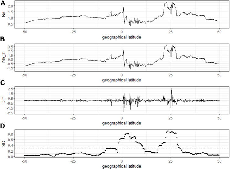
FIGURE 1. Demonstration of irregularity detection process (A) Original nighttime orbit Ne (unit:×104/cm3) measurements along the geographical latitude; (B) normalization of the orbit Ne measurements; (C) first-order differentiation of the normalized Ne measurements; (D) standard deviation of the differentiation.
The outline of the method is as following.
1) Standardize the in situ Ne measurements along the orbit, as shown in Figure 1B, so that a unified criterion on determining irregularity event can be applied to all the orbit measurements.
2) Calculate the first-order differentiation on the normalized measurements in step (1) to remove trends existed in the orbit measurements over a large latitude range. The result is shown in Figure 1C.
3) Calculate the standard deviation (SD) of a slipping window using the first-order differentiation series in step (2) and determine irregularity event with a given SD threshold criterion, the dashed line shown in Figure 1D.
4) An irregularity event is determined for continual SDs greater than the threshold value (TV). Two events are detected in Figure 1D for SDs above the dashed line. The location of the event is decided using the average latitude and longitude of the SDs ≥ TV; and the intensity of the event is decided using the average SDs. Therefore, SD with a bigger value indicates irregularity with relative large amplitude fluctuation, namely, large SD means strong irregularity intensity.
This detecting method is generally similar to the method by Beshir et al. (2020), the only difference is that the normalization process in this study is performed on the original track measurements, while in the paper by Beshir et al. (2020) the normalization process is performed on the deviation. In essence, the final results are similar for the two methods.
An explanation is given here that how to select the threshold value depends on the objective of the work. If a smaller threshold is adopted, more irregularity events will be detected; in contrast, with a relative larger threshold value, less irregularity events can be identified. Different threshold values are examined in this study and also in another study (Wang et al., 2022), and all the results show similar statistical features, indicating that the number of detected irregularities does not change the spatiotemporal statistical properties.
Based on the Ne measurements from the orbit tracks mentioned in Section 2.1, the background Ne is also calculated to compare with the irregularity distributions. The background Ne is obtained by averaging the Ne measurements in a time window and a geographical latitude and longitude grid of 2°×5°. The process to calculate the background Ne is as following (Wang et al., 2021a).
1) The space near the equator (geographical latitude of ±30°) is divided into 2°×5° grids according to the latitude and longitude spatial resolution.
2) In each grid, select all the Ne measurements from the orbits in a pre-defined time window, and a data series is obtained.
3) The Ne measurements lower than 1/4 quantile and higher than 3/4 quantile are removed from the data series; and the mean Ne is calculated only using the remaining Ne measurements in the data series. By this way, large data fluctuation, such as that induced by irregularities (Ne with much lower values) or induced by geomagnetic activities (Ne with higher values), can be reduced from the mean Ne, so that the background Ne will change smoothly.
4) Iterate over each grid to get the background Ne of all grids.
To compare with the corresponding irregularity distributions, the 3 months (seasonal) and 12 month (yearly) background Ne are calculated using the method given above.
The solar activity index F10.7 and geomagnetic activity index Dst during 2019–2021 are given in Figure 2. It can be seen clearly from Figure 2A that the solar activity level is extremely low in 2019, and begins to increase from about October 2020. In addition, there are only a few very small geomagnetic activity events (Dst<−30 nT) during the study period as shown in Figure 2B except the relatively bigger one (Dst<−100 nT) in November 2021. As geomagnetic activities generally inhibit irregularity generation (Aaron, 1982; Singh et al., 1997), we therefore use all the observations without excluding the data obtained during geomagnetic activities.
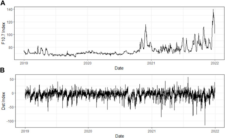
FIGURE 2. Time series of F10.7 and Dst indices from 2019 to 2021. [(A) F10.7 Index; (B) Dst Index].
According to Figure 2, the overall solar activity level in 2019 is generally constant, with a very low F10.7 index. Therefore, in situ Ne measurements in 2019 are used in this section to demonstrate the spatiotemporal distribution and seasonal variation to avoid biases caused by different solar radiation and to perform statistics under similar conditions.
Spatiotemporal distribution of the irregularity events in 2019, detected using the method described in Section 2.2 with a threshold value of 0.15, is given in Figure 3, which covers the ±30° geographical latitude near the Equator. The region between ±20° geomagnetic latitudes (shown as red dashed lines) is chosen as the near equatorial region following the conventional approach adopted by previous studies. It should be noted that geomagnetic coordinates here are converted from the IGRF12 coordinates at the altitude of the CSES satellite using the geographical coordinates of the detected irregularity events, as only the geomagnetic dipole coordinates are provided in the original Ne dataset. The geomagnetic dipole coordinates are different from those of the IGRF model, such as the geomagnetic dipole equator (black solid line) and the IGRF dip equator (black dashed line) shown in Figure 3, a large discrepancy can be seen between the two equators in longitudes from American to African sector. Therefore, IGRF geomagnetic latitudes are used when performing statistics related to the geomagnetic coordinate.
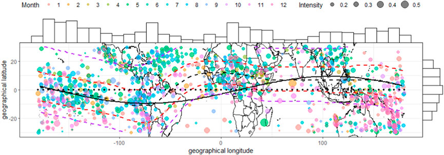
FIGURE 3. Spatiotemporal distribution of irregularities in equator and its adjacent regions in 2019. (Each irregularity event is represented by a dot. The irregularity intensity is represented by the dot size, and occurrence month is represented by dot colors. The dotted line is the Equator, and the black solid line is the dipole geomagnetic equator provided in the original dataset. The dashed lines are dip latitudes at the satellite altitude obtained from the IGRF12; the black dashed line is the dip equator, the red lines ±20° dip latitudes, and the purples lines ±35° dip latitudes).
In Figure 3, also given are the histograms of these irregularity events, representing density variations of the irregularities along with geographical longitude and with IGRF geomagnetic latitude, which are placed above and to the right of the spatiotemporal distribution plot, respectively. The histograms are drawn using the events within ±20° IGRF dip latitudes, i.e., the irregularity events within the two red dashed lines in Figure 3.
In Figure 3, each dot represents an irregularity event with the color indicating the occurrence month and the size its intensity; the larger the dot, the stronger the intensity of the irregularity event. The solid black line is the dipole geomagnetic equator provided in the original Ne dataset, and the black dotted line is the Equator. The dashed lines are dip latitudes obtained from the 12th IGRF model at the CSES orbiting altitude, with the black dashed line representing the dip equator, the red dashed lines the ±20° dip latitudes, and the purple dashed lines the ±35° dip latitudes.
It can be seen clearly from Figure 3 that, besides the equatorial regions between the two red dashed lines, the irregularities are also concentrated in two regions beyond the equatorial region, which are in the longitude sectors where the geomagnetic poles are located, and on the hemisphere close to the geomagnetic pole (around longitude −72° in northern hemisphere and 107° in southern hemisphere according to information from the NOAA website: https://www.ncei.noaa.gov/products/geomagnetism-frequently-asked-questions, latest access 2023-5-19). In fact, the post-midnight irregularities can be found throughout the satellite spatial coverage according to Wang et al. (2022), indicating that post-midnight irregularities are frequently occurred phenomenon during LSA period. As the equatorial irregularities are the focus of this paper, we will concentrate on the data between the two red dashed lines in Figure 3.
As shown in Figure 3, the equatorial irregularities are distributed well along the dip equator, i.e., the black dashed line in the figure; and the geomagnetic latitude distribution of the equatorial irregularities is symmetrical about the dip equator, as shown in the histogram to the right of the spatiotemporal distribution plot. An obvious wavenumber pattern is shown along geographical longitude in the spatial distribution and in the histogram above it, with the African, Asian, Central Pacific, and West American longitude sectors being the peak and the Indian, West Pacific, East Pacific, and Atlantic longitude sectors being the valley of the wave structure. It should be noted that the Atlantic longitude sector is a valley of the wave structure with only a few irregularity events. The low number of irregularities in the Atlantic longitude sector is quite different from previous findings that the Atlantic sector is a region of concentrated post-sunset irregularities (Maruyama and Matuura, 1984; Kil and Heelis, 1998; Huang et al., 2001; 2002; Burke et al., 2004; Su et al., 2006), which will be discussed in Section 4.
Among the four longitude irregularity peaks, three are very obvious, generally distributed symmetrically on the two sides of the dip equator, including the peaks in the Central Pacific, West American, and African longitude sectors, where the geomagnetic declination is eastward or close to zero. The one exception is the distribution peak in Asian longitude sector. This peak is not obvious as the three mentioned above from the longitude distribution of the equatorial irregularities as given in the histogram on the top of the spatiotemporal distribution plot in Figure 3. Irregularities of this longitude sector are obvious concentrated in the northern hemisphere, which forms an irregularity peak in spatial distribution. However, due to the selection criterion of the 20° dip latitude, most of the irregularities are removed from the statistics and result in the smaller peak of this longitude sector. Similar to this situation, the irregularities in the West Pacific longitude sector are mostly located in the southern hemisphere and forms another spatial concentration, with most of the irregularities being beyond the −20° dip latitude. It can be seen clearly from Figure 3 that the occurrence season is contrary for the two irregularity concentrations (the Asian and West Pacific regions).
Besides the two regions, the seasonal variation of the equatorial irregularities are also very obvious in Figure 3, with most of the events occurring during the summer months of each hemisphere, i.e., for most of the irregularity events in Northern Hemisphere, the occurrence time is northern summer, and most of the events in Southern Hemisphere, the occurrence time is southern summer (northern winter), as mentioned above that events in the Asian sector is in summer and in the West Pacific peaks is in winter. To show this seasonal feature, the histogram of equatorial irregularities in each month is given in Figure 4.
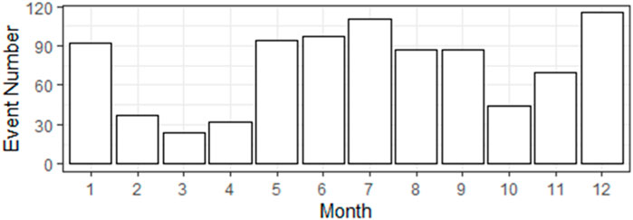
FIGURE 4. Monthly variation of the equatorial irregularities in 2019.
Two peaks and two valleys are shown in the monthly histogram of the equatorial irregularities in Figure 4, with most of those events being concentrated in the two solstice periods and less events in the two equinox periods. Another feature of the seasonal variation is that the summer peak lasts a longer time compared to the winter peak, extending from summer to the autumn season; while the winter peak is only evident at the winter solstice, with a tendency of extending towards February.
To get the seasonal variation of each longitude sector, the equatorial region is divided into 12 sub-regions with a longitude interval of 30°. The monthly variation of each sub longitude regions is given in Figure 5. In Figure 5, numbers from 1 to 12 shown above each plot represent longitude sector (−180,−−150), (−150,−120), (−120,−90), (−90,−60), (−60,−30), (−30,0), (0,30), (30, 60), (60, 90), (90, 120), (120, 150), and (150, 180) respectively.
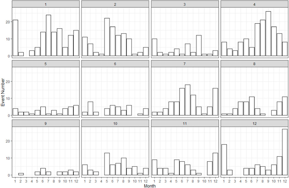
FIGURE 5. Monthly variation of equatorial irregularities in each longitude sector (Numbers from 1 to 12 above each plot represent longitude regions from −180° to 180° with an interval of 30°. Namely, 1-(−180,−150); 2-(−150,−120); 3-(−120,−90); 4-(−90,−60); 5-(−60,−30); 6-(−30,0); 7-(0,30); 8-(30,60); 9-(60,90); 10-(90,120); 11-(120,150); 12-(150,180).).
As can be seen from Figure 5, a generally similar pattern of seasonal variation peaking in summer, winter, or both seasons is shown in each longitude sector. Seasonal variation pattern is more obvious in longitudes where irregularity peaks are located in Figure 3, such as Region 1 and 2 (the Central Pacific longitudes), Region 4 (the West American longitudes), Region 7 (the African longitude), and Region 10 (the Asian longitudes). Region 12 indicates the irregularity concentration in the West Pacific longitudes in Southern Hemisphere, demonstrating a winter seasonal pattern. Compared to the peak longitudes, seasonal variation pattern is not so obvious for irregularity valley longitudes as there are only a few irregularity events, such as Region 3 (the east Pacific longitudes), Region 5 and 6 (the East American and Atlantic longitudes), Region 9 (the Indian longitudes). Further statistics using irregularities detected with a lower threshold of 0.1 indicates a summer or winter seasonal pattern in the irregularity valley longitude sectors.
Though the general seasonal variation is summer or winter peak in each longitude sector, the time when the peaks appear and the relative amplitudes of the two peaks are varying gradually. Examples of this gradual seasonal variation with longitude are that only the summer peak appears in longitude sector of 90°–120° (Region 10); in contrast, only the winter peak occurs in longitude sector of 150°–180° (Region 12); and both summer and winter peaks can be seen in the longitude sector of −180° to −150° (Region 1).
Summarizing the above analysis, the spatiotemporal distribution features are that the equatorial post-midnight irregularities are generally distributed symmetrically about the dip equator, exhibiting a wavenumber 4 pattern along the dip equator, and their general seasonal variation pattern is solstice peaks and equinox valleys with a general gradual variation from one solstice peak to both solstice peaks.
To compare the distribution of equatorial post-midnight irregularities with its background Ne, the seasonal background Ne distributions are plotted using the results calculated from the nighttime in situ Ne measurements in the four seasons of 2019. The background Ne calculation method is introduced in Section 2.3. The four seasons are divided in the normal way, i.e., February, March, and April belong to the March Equinox, May, June, and July the June Solstice, August, September, and October the September Equinox, and November, December, and January the December Solstice.
The background Ne (unit:/cm3) distributions for the four seasons and their corresponding irregularity events are presented in Figure 6. Each event is represented by a dot with its size indicating the intensity of the irregularity, similar as that in Figure 3.
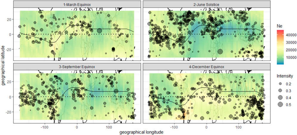
FIGURE 6. Comparison of background Ne and irregularity distribution in different seasons. (The unit of Ne is/cm3).
As can be seen from Figure 6, a general wavenumber pattern is shown in the seasonal background Ne distributions with a typical wavenumber of 3 or 2. In addition, it is clearly shown in Figure 6 that the peak and valley positions of the wavenumber pattern vary with seasons as well as with the wave number. Wavenumber 2 pattern is obvious for the two solstice seasons with the African and the Pacific-West American longitude sectors being the peaks for the June solstice and the Central Pacific and the American-Atlantic-African longitude sectors being the peaks for the December solstice; and wavenumber 3 pattern is obvious for the two equinox seasons with the Asian, the Central pacific, and the American-African longitude sectors being the peaks for the March Equinox and the African, the Central Pacific, and the West American longitude sectors being the peaks for the September Equinox. With the position variation of the background Ne peaks, the irregularities peaks also change their positions. The irregularity peaks generally coincide with the background Ne peaks in different seasons.
As a further comparison, Figure 7 gives the yearly distribution for background Ne and irregularity events in 2019. As mentioned above, the African, the Central Pacific, and the West American longitude sectors have been the background Ne peaks for all the seasons, as a result they are also the yearly background Ne peaks. Since the seasonal irregularity peaks coincide with the corresponding background Ne peaks, the yearly irregularity peaks are also coincide with that of the yearly background Ne peaks. Relatively higher background Ne appears in the Asian and the West Pacific longitude sectors on both side of the dip equator, where irregularities are correspondingly more concentrated. Though the Central Pacific to the West American longitude sector shows a continuous Ne peak in Summer solstice, a valley can be seen clearly in the West Pacific longitude sector for the other three seasons, as shown in Figure 6. Combining the background Ne of the four seasons together, a valley can be seen clearly between the Central Pacific and the West American longitude sector in the yearly background Ne distribution in Figure 7, which corresponds also to a relative irregularity valley.

FIGURE 7. Comparison of yearly background Ne and irregularity distributions in 2019 (The unit of Ne is similar as that of Figure 5).
Both the seasonal and yearly distributions for background Ne and post-midnight irregularities show that the two (background Ne and post-midnight irregularity) have similar wavenumber distribution pattern along the longitude direction, suggesting that post-midnight irregularity distribution is closely related with the background Ne distribution.
Through the comparison of the seasonal and yearly background Ne and irregularity distributions, coincidence of the two is shown in longitude distribution and peak locations. A preliminary conclusion can be drawn that the distribution of topside background Ne obviously affects the distribution of post-midnight irregularities during LSA period, that is, the background Ne distribution plays an important role in the generation of post-midnight irregularities. See Section 4 for a further discussion of this topic.
Solar activity in 2019, 2020, and 2021 belongs to LSA in general. However, it can be seen clearly that the solar activity level has begun to increase since October 2020 in Figure 2. Therefore, irregularities detected in different month of the 3 year 2019, 2020, and 2021 can be compared to obtain the influence of solar activity on the generation of post-midnight irregularities in the topside ionosphere. Figure 8 gives the variation of monthly irregularity occurrence rate with solar activity represented by monthly average F10.7 index. The monthly occurrence rate is calculated as the ratio between orbits with irregularities in a month and total orbits in that month.
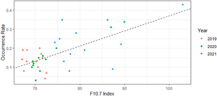
FIGURE 8. Variation of irregularity occurrence rate with solar activity. (The dashed line is the linear fitting between occurrence rate and F10.7 Index).
It is clearly shown in Figure 8 that post-midnight irregularity occurrence rate increases with increasing solar activity, with a Pearson significant correlation coefficient of 0.68, indicating a significant correlation. In general, occurrence rate is relatively high in 2021 (blue dot), and occurrence rate in 2020 (green dot) is generally similar to that in 2019 (red dot), except 2 months. To show more detailed information, Figure 9 compares the monthly variation of irregularity occurrence rates and F10.7 index. In spite of the different solar activity, an obviously seasonal variation pattern of Summer-Winter peak and Spring-Autumn valley is shown clearly in Figure 9. The 2 months with high occurrence rate in 2020 in Figure 8 correspond to November and December when the solar activity increases suddenly in Figure 9; and the F10.7 index in 2021 is generally high compared to 2019 and 2020, which corresponding to the relatively high occurrence rate in 2021 in Figure 8. Variation of occurrence rate with solar activity indicates that solar activity can affect the generation of post-midnight irregularities just as it does on post-sunset irregularities.
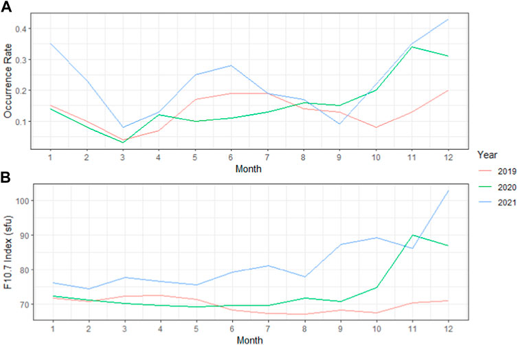
FIGURE 9. Comparison of irregularity occurrence rates and solar activities in 2019, 2020, and 2021. [(A) Monthly occurrence rate; (B) Monthly average F10.7 Index].
The above analysis indicates that occurrence rate of post-midnight irregularity generally shows an increase trend with the increasing solar activity. Due to the very low solar activity during the study period, it is not possible to draw a definite conclusion on the variations of the post-midnight irregularity occurrence rate with solar activity as the data does not even cover half of a solar cycle. However, the results obtained from the 3 years Ne measurement do indicate that solar activity can influence the occurrence rate of post-midnight irregularity even under LSA conditions.
To exam whether different longitude sectors are equally influenced by the increasing solar activity, a further comparison is conducted using the irregularity events detected in October, November, and December of the 3 years in different longitude sectors. Twelve longitude sectors are divided in the equatorial regions with a longitude interval of 30° as it does in Section 3.1. The result is shown in Figure 10.
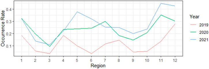
FIGURE 10. Irregularity occurrence rate in October, November, and December of the 3 years in different longitudes (The x-axis uses numbers to indicate different longitude sectors, and the numbers represent: 1-(−180,−150); 2-(−150,−120); 3-(−120,−90); 4-(−90,−60); 5-(−60,−30); 6-(−30,0); 7-(0,30); 8-(30,60); 9-(60,90); 10-(90,120); 11-(120,150); 12-(150,180).).
Comparing the occurrence rates in each longitude sector in Figure 10 indicates that the maximum growth of occurrence rate is in Region 5 and 6, corresponding to longitude −60°–0°, where is just the Atlantic longitude sector; and followed by Region 11 and 12, corresponding to longitude 120°–180°, in the Australian and the West Pacific regions in Southern Hemisphere. The longitude variation of growth rate of irregularity occurrence rate with increasing solar activity suggests that increasing solar activity has different effects on the generation of post-midnight irregularities in different longitude sectors. If this effect continues to exert influence with the increasing solar activity, it is conceivable that the spatial distribution may change from its wavenumber 4 distribution pattern in Figure 3 to other distribution patterns, such as changes in peak positions or in total wave numbers. For example, variation of peak position is evidently shown in Figure 10; the maximum occurrence place is located at Region 12 in 2019, and it changes to Region 11 in 2020 and 2021; and moreover, the peak region seems to widen, occupying both Region 11 and 12. Clues of variation of wavenumber pattern can also be seen in Figure 10. Three occurrence peaks can be seen in 2019 using the detected irregularity results in October, November, and December; however, there seems only two occurrence peaks in 2021 and 2022 using the results obtained in the same 3 months. Due to the variation of peak position and wave number with solar activity, the Atlantic longitude sector becomes a peak in 2020 and 2021 from the valley in 2019.
The above analysis suggests that even under LSA conditions, solar activity can obviously affect the generation of post-midnight irregularities. Moreover, this influence is different in different longitude sectors, which will further affect the longitude distribution of irregularity occurrence with the Atlantic longitudes being the most affected region during the study period.
Post-midnight irregularities during very low solar activity period are studied using the in situ Ne measurements obtained by the CSES satellite orbiting at an altitude of 507 km, to analyze their spatial distribution and seasonal variation features in the topside ionosphere. The results show that a general wavenumber 4 distribution pattern is shown for the post-midnight irregularities with a seasonal variation of summer-winter peaks and spring-autumn valleys. The peaks of irregularities longitude distribution in the four seasons coincide with the peaks of the corresponding background Ne distribution in that season with a general wavenumber 3 pattern for equinox seasons and wavenumber 2 pattern for solstice seasons; a wavenumber 4 longitude variation pattern is shown along the dip equator when combining the irregularities in the four seasons, which also coincides with the corresponding yearly background Ne distribution. Results, obtained by comparing the occurrence rate under different solar flux during LSA period, show that post-midnight irregularity occurrence rate increases with the increasing solar flux and different longitude sectors exhibit different growth rate of occurrence rate with the increasing solar activity; the maximum growth rate is located at the Atlantic longitude sector, followed by the Australian to West Pacific longitude sector. These features suggest that solar activity exerts influence on the generation of post-midnight irregularities although the general solar activity condition remains at LSA level.
For the above results obtained in this paper, some issues need to be clarified, and the related discussions are given in the following section.
The longitudinal/seasonal variation of the post-sunset equatorial irregularities have been investigated extensively over the past decades (Maruyama and Matuura, 1984; Tsunoda, 1985; Whalen, 1997; McClure et al., 1998; Huang et al., 2001; Huang et al., 2002; Burke et al., 2004; Gentile et al., 2006; Su et al., 2006; Su et al., 2008), such as: Huang et al. (Huang et al, 2001, Huang et al, 2002) report that seasonal and longitudinal variations of post-sunset irregularities remain similar within given longitude sectors using the DMSP measurements over a full solar cycle; they suggest that the Atlantic-African sectors are the most significant occurrence longitudes and the Indian sector is the least occurrence longitudes. Burke et al. (2004) also show that the highest and lowest rates of equatorial plasma bubble (EPB) located at the Atlantic-African and Indian sectors using both the DMSP and the ROCSAT-1 measurements. Kil and Heelis (1998) suggest that scintillation is always high in the Atlantic-African longitudes and is always low in the Indian regions.
The spatiotemporal structures of post-midnight irregularities are also reported by a few studies. For example, Su et al. (2018) report that the post-midnight irregularity distribution is similar to the pre-midnight ones using the in situ measurements from ROCSAT-1 satellite obtained during moderate to high solar activity years of 1999–2004, with the African and Central Pacific sectors being the high occurrence places for June solstice, and the South America and the Atlantic Ocean sectors being the high occurrence place for December solstice. Dao et al. (2011) and Yizengaw et al. (2013) find the longitudinal structures using the C/NOFS in situ measurements obtained in LSA years; they also find that the maximum occurrence is located at South American and African sector sectors for summer solstice months, and significant activity occurs at Pacific and South American longitude sectors for winter solstice months.
The above post-sunset and post-midnight irregularity longitude distribution results are general in agreement with the spatiotemporal distribution obtained in this study, with the exception of the Atlantic sector, which is a low occurrence region for the post-midnight irregularities detected in 2019. However, the subsequent results of this study further demonstrate that irregularities in the Atlantic longitude sector increase dramatically, and this region becomes the peak with the increasing solar flux as shown in Figure 10. In fact, the solar flux remains at LSA for the entire study period though it has been increasing since October 2020. Therefore, the general longitude distributions for both post-sunset and post-midnight irregularities are consistent with each other.
It should be pointed out here that the low irregularity occurrence in the Atlantic longitude sector in 2019 does not mean the result is not correct. In fact, this low occurrence rate of post-midnight irregularities in the Atlantic longitude sector is also noticed by Dao et al. (2011) using the C/NOFS measurements from May 2008 to March 2010, an extremely prolonged LSA period between 23/24 solar cycle. Our result is in agreement with that of Dao et al. (2011), indicating the result in this study is correct and can be replicated from different datasets under similar solar activity conditions. The facts that low occurrence rate in 2019 but relatively higher occurrence rate in 2020 and 2021 shown in the post-midnight irregularities indicate that rather different features can appear in the Atlantic longitude sector under generally similar conditions, suggesting that the post-midnight irregularities in topside ionosphere are very sensitive to solar flux variation under LSA conditions, which may be closely related with the low geomagnetic field in the South Atlantic Anomaly (SAA) region. More studies are required to further analyze the mechanism behind the phenomenon.
As to the wave-like structure of post-midnight irregularities and its coincidence with the wave-like background Ne, a simple explanation is given here. According to the study by Sidorova and Filippov (2018), the wave-like structure for post-sunset irregularities is influenced by troposphere tide and associated with the troposphere DE3 tides, which affect the thermosphere parameters and ionosphere parameters through the modulation of the thermosphere winds and electric fields. In addition, Beshir et al. (2020) suggest that strong plasma densities result in stronger post-sunset irregularities, while relatively less dense plasma results in relatively lower irregularities. The coincident results in this study indicate that post-midnight irregularities may also be influenced by the troposphere tides, and the background Ne controls the distribution of post-midnight irregularities. Thus, the low occurrence in 2019 in the Atlantic longitude sector must be related to the extremely low background Ne in this region.
In summary, comparisons of the longitude variation for post-midnight and post-sunset irregularities indicate they have similar wave-like structure. Moreover, the concentrated irregularities coincide with the background Ne peaks. Both these features suggest that some places provide persistent favorable conditions for the generation of equatorial irregularities, independent of the nighttime irregularity occurrence time and season. Furthermore, the background Ne plays an important role in the generation of nighttime irregularities during LSA period.
The general seasonal variation pattern of the post-midnight equatorial irregularities obtained in this study is summer-winter peaks with spring-autumn valleys, as shown in Figure 4. This seasonal variation pattern is in agreement with the results obtained by Heelis et al. (2010) using the C/NOFS in situ measurements observed under extremely LSA conditions in 2008 and 2009. Their results show that post-midnight occurrence frequency peaks during both northern winter and summer period, but is very low during equinox period.
The seasonal variation pattern for post-midnight irregularities is quite different from the equinox peaks and solstice valleys pattern of post-sunset irregularities reported by many previous studies (Tsunoda, 1985; Huang et al., 2001; Huang et al., 2002; Burke et al., 2004; Hei et al., 2005; Su et al., 2006; Su et al., 2008). Based on the long-term ground-based measurements in India, Sastri (1999) reports that post-sunset spread F occurrence peaks in equinox months during high solar activity (HSA) period; and during LSA period, post-midnight spread occurrence peaks in solstice months. Otsuka et al. (2009) also report that irregularities appear frequently at pre-midnight between March and May and at post-midnight between May and August using ground-based measurements in Indonesia in a relatively LSA period. Miller et al. (2010) find that more irregularities appear later in the winter evening during LSA period in the Pacific longitude sector. Candido et al. (2011) also find the solstice peaks seasonal variation pattern in Brazil. All these studies, using long-term ground-based measurements in different longitudes, show that the peak seasons and LTs of nighttime irregularity occurrence vary with solar activity. These results obtained from ground-based measurements are similar to the seasonal and LT variations of nighttime irregularities obtained from satellite-based measurements. For example, some studies, using the C/NOFS satellite measurements obtained during solar minimum of cycle 23/24, report the shift of peak occurrence from post-sunset hours during HSA period to post-midnight hours during LSA period (Yokoyama et al., 2011; Yizengaw et al., 2013). All studies using ground-based and satellite-based ionospheric irregularities suggest that post-midnight irregularities are very common phenomenon for both the bottomside and topside ionosphere with similar seasonal variation pattern, and there may be a close relationship between irregularities generated at bottomside and topside ionosphere.
Since generation of irregularities is associated with the ionosphere dynamical processes, we believe that the variations of irregularity peak season and peak LT with solar activity can indicate the variation of ionosphere dynamical processes with solar activity. Therefore, issues related with irregularity seasonal and LT variations deserve more research work. As to how to connect the different seasonal variations between irregularities generated at post-midnight and post-sunset, it is necessary to obtain more simultaneous satellite-based measurements from different LTs to gain in-depth knowledge, and this work is under construction.
Solar activity dependence of post-sunset irregularity occurrence has been reported by many previous studies (Abdu et al., 1985; Huang et al., 2002; Nishioka et al., 2008; Su et al., 2008). The results in this study indicate that post-midnight irregularities are also closely related to solar activity. Variation of post-midnight irregularities with solar activity shows an increasing trend with the increasing solar flux. However, this does not mean that post-midnight irregularity will always follow this trend. In fact, the general trend is that post-midnight irregularities decrease as solar activity increases, according to the study by Fejer, (1999) based on long-term ground-based measurements. They attribute the decrease in post-midnight irregularities to the large increase of the nighttime downward drifts with the increasing solar flux, which will be discussed further in the next section.
How can we explain the result obtained in this study that post-midnight irregularities increase with increasing solar flux during the study period? Two reasons are given below.
On the one hand, although solar activity has been increasing since October 2020 as shown in Figure 2, the overall solar activity remains very low in 2020 and 2021 with the overall monthly average F10.7 index being less than 100sfu (sfu is the solar flux unit, 1 sfu = 10–22 W m−2 Hz−1), which is in the range of LSA level according to the criteria used in previous studies (Huang et al., 2002; Nishioka et al., 2008).
On the other hand, electron density is sensitive to solar flux, especially under LSA conditions (Liu et al., 2011). As in the case of 2019 shown in Figure 8, the monthly average solar flux is around or below 70sfu, which is particularly low. Under this solar condition, increasing solar flux leads to the obvious increases of Ne, and therefore the increase of post-midnight irregularities. To demonstrate the relation between irregularities and Ne, Table 1 gives the average F10.7 index and average nighttime Ne as well as irregularity occurrence rate from October to December in 2019, 2020, and 2021, using the measurements in the geographical longitude range of −50° to −20° and in the dipole geomagnetic latitude range of −10°–10°, which belongs to the equatorial Atlantic region.
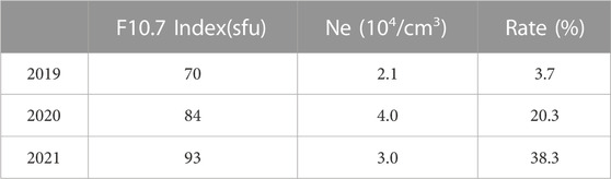
TABLE 1. Average F10.7 index, Ne, and irregularity occurrence rate in the Atlantic region.
Ne and irregularities increase much faster than the F10.7 index, and in this case the rapid increase of irregularities is more related to Ne than to solar flux. It is worth noting in Table 1 that irregularity occurrence rate keeps increasing in 2020 and 2021 with the increasing F10.7 index, however the Ne in 2021 decreases compared to that in 2020. How to explain it? As the Ne is calculated by averaging the Ne measurements in the selected grid and time window, the average Ne will be lowered when more Ne measurements with irregularities are involved in the calculation due to the extremely low values of these Ne measurements.
The close relation between Ne and irregularities suggests that background Ne plays very important role in the generation of post-midnight irregularities, which is consistent with the suggestion obtained by Basu et al. (1988) that the drastic reduction of post-sunset scintillation occurrence from solar maximum to solar minimum indicates that the background density is the major modulating factor. It is easy to understand that large density fluctuation cannot be produced when the background density is very low; and as a result, there will be fewer irregularities (Dymond, 2012). When the background density condition is satisfied, irregularities increase rapidly in the longitude sectors where they are easy to generate.
When it comes to the places prone to irregularities, another interesting phenomenon caused by the enhancing solar activity is that the growth rate of irregularity occurrence rate with increasing solar activity is markedly different across different longitudes, with the Atlantic and Pacific longitude sectors being the two most significant regions, where are the places both post-sunset and post-midnight irregularities frequently occur as mentioned in Section 4.1. To demonstrate this characteristics, Figure 11 gives the spatiotemporal distributions of irregularities detected in 2020 and 2021.

FIGURE 11. Spatiotemporal distribution of equatorial irregularities in 2020 and 2021. [The symbols in Figure 11 are the same as in Figure 3; (A) is the data for 2020, and (B) for 2021].
As solar activity increases most significantly during the winter season, more irregularities occur at the southern hemisphere for 2020 and 2021. Due to the increasing irregularities, the wavenumber 4 pattern can be recognized in 2020, but it is not obvious in 2021 as the irregularity valley in the Atlantic longitude sector is concentrated with irregularities. It can be seen clearly that irregularities in the Atlantic and Pacific longitude sectors increase faster than it does in other longitude sectors. The unbalanced increase of irregularities in different longitude sectors leads to the variation of wavenumber pattern as suggested in Section 3.3. In fact, unbalanced increases of irregularities with increasing solar activity is also noticed by Nishioka et al. (2008); they suggest that the Atlantic, African, and Asian longitudes are the regions suffered the most significant influence, which is generally consistent with our results. This consistency further suggests that post-midnight irregularities have similar features to those of post-sunset irregularities.
As the reasons for the unbalanced increase of irregularities are beyond the scope of this study, we leave this question here; more studies will be conducted on this topic in our subsequent work.
Using irregularities data obtained from ground-based measurements, Otsuka (2018) suggests the generation conditions for the F2 layer post-midnight irregularities: 1) seeding of the Rayleigh-Taylor instability (RTI) by atmospheric gravity waves (AGWs) propagating from stratosphere into the ionosphere, and 2) Uplifting of the F layer helps to generate altitude gradient and is favorable to the ionosphere instability. The AGWs seeding factor is also investigated by Seba et al. (2021), and their results indicate that AGWs and irregularities are closely related.
As the focus of this paper is post-midnight irregularities in topside ionosphere, the altitude of the topside ionosphere (507 km) is about 200 km or more away from the F2 layer maximum height (hmF2) compared to the average hmF2 (250–300 km) (Otsuka, 2018) during LSA period, where post-midnight irregularities during solstice seasons are found frequently from ground-based measurements in solar minimum years. In addition, Dao et al. (2016) find that the post-midnight irregularities in the F2 layer generate after sunset time, which indicates that the PRE (pre-reversal enhancement of ionosphere) condition necessary for the post-sunset irregularities does not exist for the post-midnight irregularities. Therefore, Otsuka, (2018) propose the AGWs seeding factor and the uplifting of the F2 layer generation conditions for the post-midnight irregularities in F2 layer.
Based on the facts obtained from previous post-midnight irregularity studies using ground-based measurements and the close relationship between irregularities generated at bottomside and topside ionosphere proposed in Section 4.1.2, we suggest that post-midnight irregularities generated in the F2 layer may be one of the origin for the post-midnight irregularities in topside ionosphere, but this origin cannot account for all the irregularities in topside ionosphere. The reasons are as followings.
As mentioned above, results obtained in previous studies using ground-based measurements indicate that post-midnight irregularities generated at the bottomside of ionosphere mainly appear at the hmF2 (Ajith et al., 2016; Ostuka, 2018), and most of these irregularities do not exceed 450 km (Dao et al., 2016), indicating that only a small part of the F2 layer irregularities with large scale size can reach a higher altitude considering that small-scale irregularities will survive shorter time compared to large-scale irregularities. In addition, the generation time of these irregularities are clustered around 22:00LT to 03:00LT (Ajith et al., 2016; Dao et al., 2016). As the rise velocities of post-midnight irregularities are smaller compared to those of post-sunset irregularities (Dao et al., 2016), a time delay of 1 hour to several hours is required for the irregularities in F2 layer to reach the topside ionosphere, and some irregularities cannot survive this time delay. For these reasons, only large-scale irregularities in F2 layer can reach the CSES orbiting altitude and be observed by the Ne measurements. However, this origin cannot account for the small-scale irregularities which occupy the majority of the detected events. We therefore suppose that small-scale irregularities may be generated at the topside ionosphere.
As discussed in Section 4.1 and Section 4.2, the similar spatial distribution and association with background Ne as well as response to the variation of solar activity for both post-midnight and post-sunset irregularities suggest that the two have similar generation mechanism. This suggestion is also supported by the modeling results by Yizengaw et al. (2013) that post-midnight irregularities are initiated in the same way that the post-sunset irregularities are generated. Gentile et al. (2011) also suggest that the occurrence condition of post-midnight irregularities is closely related to the upward drift velocities as it does with the post-sunset irregularities.
As is well accepted, the post-sunset equatorial irregularities, known for its characteristics of fast growth after sunset during equinox seasons, result from plasma dynamic process initiated from the gravitational Rayleigh-Taylor (R-T) instability at the bottomside of ionosphere after sunset when pre-reversal enhancement (PRE) of eastward electric field occurs due to the high conductivity gradient across the day night terminator during the post-sunset hours, leading to the sudden increase of plasma upward drift (Tsunda, 1985; Farley et al., 1986). Upward drifts can then carry the lower density at the bottomside of ionosphere to altitudes with higher density, leading to the generation of irregularity structures in F2 layer.
As the post-sunset equatorial irregularities are generated due to the seeding factor of PRE with an unstable conditions at the bottom of F layer, however, these favorable conditions are absent after midnight in the topside ionosphere. Therefore, two problems need to be addressed if post-midnight irregularities are assumed to generate in topside ionosphere and have similar generation mechanism as the post-sunset irregularities. The first problem is the instability condition for the topside ionosphere. As this condition is always satisfied at the bottom side of the ionosphere F layer due to the lower plasma density compared to higher altitudes, how to satisfy this condition in the topside ionosphere? The second problem is the upward drift condition. It is well known that nighttime electric field after PRE is general westward, which causes plasma to drift downward. Reversal of electric field from westward to eastward is required to satisfy the seeding condition for topside ionosphere if we assume that post-midnight irregularities are generated under the similar conditions as that of the post-sunset irregularities.
The first problem can be solved based on the results obtained in our previous studies. According to the results by Wang et al. (Wang et al. 2019b; Wang et al. 2020), nighttime stratification, which indicates that Ne is greater in higher altitudes than in lower altitudes above hmF2 height, is frequently found in the topside nighttime ionosphere near the equatorial regions during LSA period, which provides the R-T instability condition for the topside ionosphere, favoring the generation of irregularities at this altitude. Detailed information on nighttime stratification in topside ionosphere is beyond the scope of this paper and will be discussed in a separate paper.
For the second condition, an explanation is given as following. Gentile et al. (2011) and Yizengaw et al. (2013) prove that post-midnight occurrence condition is closely related to the upward drift velocities; Rastogi and Woodman (1978) also suggest that reversal of drift from downward to upward is the key to the generation of spread F in the ionograms. According to the results by Fejer et al. (1991), the downward plasma drift due to nighttime westward electric field is generally weak during the post-midnight hours of solstice seasons, particularly during LSA periods. Fejer and Scherlies, (1995) also report that average nighttime vertical drifts from the AE-E satellite are upward during summer solstice months in 1977 of a relative LSA year and are downward in 1978 and 1979 of moderate to HSA years. In addition, simultaneous electric field and density observations from the C/NOFS satellite prove that the electric field is eastward when irregularities are observed by the in situ density measurements (de La Beaujardière et al., 2009); we also examine some simultaneous electric field and Ne orbit measurements onboard CSES and find that electric field reversals coincide with the appearance of irregularities. All these studies suggest that nighttime irregularities are caused by upward plasma drifts and the upward drifts condition can be satisfied under LSA conditions.
As both the instability and upward drift conditions can be satisfied, it is possible that post-midnight irregularities can generate in topside ionosphere during LSA period. Moreover, irregularity generation in topside ionosphere can be explained by the R-T instability growth rate equation proposed by Sultan (1996). According to the equation, R-T instability is inversely proportional to the ion-neutral collision frequency. As ion-neutral collision frequency is extremely low due to the low density in topside ionosphere, the R-T instability growth rate will become large even when the electric field is westward. Since the vertical gradient is positive due to the existence of nighttime stratification phenomenon, it is very possible to generate irregularities in topside ionosphere as the R-T instability growth rate is very large at this altitude during LSA period.
It should be noted here that small irregularities or irregularities with smaller intensity can occur in the topside ionosphere under the above mentioned favorable conditions. As shown in Figure 3, smaller irregularities account for a large proportion of the detected irregularity events. However, for some very large irregularity structures covering a latitude range of over 20° with Ne fluctuation of close to an order of magnitude, the above conditions seem to be insufficient for these large-scale irregularity structures. Large-scale irregularities generated at F2 layer and reach the CSES orbiting altitude, mentioned in Section 4.3.1, can be used to explain these irregularities, which occupies only a very small part (about 2.7% with intensity greater than 0.5) of the detected irregularity events. Since the large-scale irregularities covering a wide latitude range always appear in the Atlantic longitude sector, they must be related to the special geomagnetic condition there. This issue, as well as the one mention in Section 4.1 concerning the Atlantic longitude sector, requires further studies.
The equatorial post-midnight irregularities are studied using the in situ electron density measurements from 2019 to 2021 obtained by the CSES satellite orbiting at the altitude of topside ionosphere during LSA period. Some results are obtained.
1) The equatorial post-midnight irregularities, distributed symmetrically about the dip equator, show a longitude variation pattern of wavenumber 4 along the dip equator, with the African, Asian, Central Pacfic, and West American longitude sectors being the peaks and the Indian, West Pacific, East Pacific, and Atlantic longitude sectors being the valleys.
2) The general seasonal variation pattern is summer-winter peaks and spring-autumn valleys for the equatorial post-midnight irregularities. This seasonal variation pattern varies gradually along the dip equator, with some longitudes showing summer solstice peak, some longitudes showing winter solstice peak, and other longitudes showing two peaks for both solstices.
3) The longitude distribution of post-midnight irregularities is similar to that of background Ne in the four seasons, with a general wave number 3 pattern for equinox seasons and wave number 2 pattern for solstice seasons. Coincidence of irregularity peaks with background Ne peaks for both seasonal and yearly distributions suggests background Ne plays very important role in post-midnight irregularity generation under LSA conditions as background Ne in the valley longitude sectors is too low to generate obvious irregularities.
4) Post-midnight irregularities is sensitive to solar activity under LSA conditions as occurrence rate increases rapidly with the increasing solar flux. Moreover, growth rate of irregularity occurrence rate is different across different longitudes, and the Atlantic and Pacific longitudes are the two regions with maximum irregularity growth rate.
5) There are two possible ways to be the origin of the post-midnight irregularities in topside ionosphere. One is the irregularities generated at the bottomside of the ionosphere that drift upward and reach the topside ionosphere; the other is newly generated irregularities in the topside ionosphere as nighttime stratification phenomenon and reversal of nighttime drifts from downward to upward at midnight hours during LSA period provide R-T instability and upward drifts conditions for the generation of irregularities in topside ionosphere.
As the generation mechanism of post-midnight irregularities is still unclear, it requires more research work. The large amount of in situ electron density measurements from the CSES satellite, as well as the simultaneous electric field measurements, provide us valuable datasets to study the issues related with post-midnight irregularities, and more subsequent work is under investigation using both the electron density and electric field measurements.
Publicly available datasets were analyzed in this study. This data can be found here: leos.ac.cn.
XW contributed to the conception of the study and wrote the manuscript. WC, XZ, and GZ collected the dataset used in the paper. QW, DY, and SX performed calculation and analysis work. JN and NZ examined the simultaneous electron density and electric field measurements to validate the electric field reversal condition. All authors contributed to the article and approved the submitted version.
This work is supported by the NSFC project (grant no. 42104159).
The authors are grateful to the reviewers for their constructive advices that have significantly improved the manuscript. This work made use of the in situ electron density measurements from the CSES mission, a project funded by China National Space Administration (CNSA) and China Earthquake Administration (CEA).
The authors declare that the research was conducted in the absence of any commercial or financial relationships that could be construed as a potential conflict of interest.
All claims expressed in this article are solely those of the authors and do not necessarily represent those of their affiliated organizations, or those of the publisher, the editors and the reviewers. Any product that may be evaluated in this article, or claim that may be made by its manufacturer, is not guaranteed or endorsed by the publisher.
Aarons, J. (1982). Global morphology of ionospheric scintillations. IEEE Proc. 70, 360–378. doi:10.1109/proc.1982.12314
Aarons, J. (1993). The longitudinal morphology of equatorial F-layer irregularities relevant to their occurrence. Space Sci. Rev. 63 (3-4), 209–243. doi:10.1007/bf00750769
Abdu, M., Sobral, J., Nelson, O., and Batista, I. (1985). Solar cycle related range type spread-F occurrence characteristics over equatorial and low latitude stations in Brazil. J. Atmos. Terr. Phys. 47 (8–10), 901–905. doi:10.1016/0021-9169(85)90065-0
Ajith, K. K., Tulasi Ram, S., Yamamoto, M., Otsuka, Y., and Niranjan, K. (2016). On the fresh development of equatorial plasma bubbles around the midnight hours of June solstice. J. Geophys. Res. Space Phys. 121, 9051–9062. doi:10.1002/2016JA023024
Basu, S., Groves, K. M., Basu, S., and Sultan, P. J. (2002). Specification and forecasting of scintillations in communication/navigation links: current status and future plans. J. Atmos. Sol. Terr. Phys. 64 (16), 1745–1754. doi:10.1016/S1364-6826(02)00124-4
Basu, S., MacKenzie, E., and Basu, S. (1988). Ionospheric constraints on VHF/UHF communications links during solar maximum and minimum periods. Radio Sci. 23 (3), 363–378. doi:10.1029/rs023i003p00363
Beshir, E., Nigussie, M., and Moldwin, M. B. (2020). Characteristics of equatorial nighttime spread F- an analysis on season-longitude, solar activity and triggering causes. Adv. Space Res. 65 (1), 95–106. doi:10.1016/j.asr.2019.09.020
Burke, W. J. (1979). Plasma bubbles near the dawn terminator in the topside ionosphere. Planet. Space Sci. 27 (9), 1187–1193. doi:10.1016/0032-0633(79)90138-7
Burke, W. J., Gentile, L. C., Huang, C. Y., Valladares, C. E., and Su, S. Y. (2004). Longitudinal variability of equatorial plasma bubbles observed by DMSP and ROCSAT-1. J. Geophys. Res. 109 (A12), A12301. doi:10.1029/2004ja010583
Candido, C. M. N., Batista, I. S., Becker-Guedes, F., Abdu, M. A., Sobral, J. H. A., and Takahashi, H. (2011). Spread F occurrence over a southern anomaly crest location in Brazil during June solstice of solar minimum activity. J. Geophys Res. 116, A06316. doi:10.1029/2010JA016374
Carter, B. A., Zhang, K., Norman, R., Kumar, V. V., and Kumar, S. (2013). On the occurrence of equatorial F-region irregularities during solar minimum using radio occultation measurements. J. Geophys Res. 118, 892–904. doi:10.1002/jgra.50089
Dao, E., Kelley, M. C., Roddy, P., Retterer, J., Ballenthin, J. O., de La Beaujardiere, O., et al. (2011). Longitudinal and seasonal dependence of nighttime equatorial plasma density irregularities during solar minimum detected on the C/NOFS satellite. Geophys. Res. Lett. 38, L10104. doi:10.1029/2011GL047046
Dao, T., Otsuka, Y., Shiokawa, K., Tulasi Ram, S., and Yamamoto, M. (2016). Altitude development of postmidnight F region field-aligned irregularities observed using Equatorial Atmosphere Radar in Indonesia. Geophys. Res. Lett. 43, 1015–1022. doi:10.1002/2015GL067432
de La Beaujardière, O., Retterer, J. M., Pfaff, R. F., Roddy, P. A., Roth, C., Burke, W. J., et al. (2009). C/NOFS observations of deep plasma depletions at dawn. Geophys. Res. Lett. 36, L00C06. doi:10.1029/2009GL038884
Dymond, K. F. (2012). Global observations of L band scintillation at solar minimum made by COSMIC. Radio Sci. 47, RS0L18. doi:10.1029/2011RS004931
Farley, D. T., Bonelli, E., Fejer, B. G., and Larsen, M. F. (1986). The prereversal enhancement of the zonal electric field in the equatorial ionosphere. J. Geophys. Res. 91 (A12), 13723–13728. doi:10.1029/ja091ia12p13723
Fejer, B. G., de Paula, E. R., Gonzalez, S. A., and Woodman, R. F. (1991). Average vertical and zonal F region plasma drifts over Jicamarca. J. Geophys. Res. 96 (A8), 13901–13906. doi:10.1029/91JA01171
Fejer, B. G., and Kelley, M. C. (1980). Ionospheric irregularities. Rev. Geophys. Space Phys. 18 (2), 401–454. doi:10.1029/rg018i002p00401
Fejer, B. G., and Scherlies, L. (1995). Time dependent response of equatorial ionospheric electric fields to magnetospheric disturbances. Geophys. Res. Lett. 22 (7), 851–854. doi:10.1029/95gl00390
Fejer, B. G., Scherliess, L., and de Paula, E. R. (1999). Effects of the vertical plasma drift velocity on the generation and evolution of equatorial spread F. J. Geophys. Res. 104 (A9), 19859–19869. doi:10.1029/1999JA900271
Gentile, A., Burke, W. J., and Rich, F. J. (2006). A climatology of equatorial plasma bubbles from DMSP 1989–2004. Radio Sci. 41, RS5S21. doi:10.1029/2005RS003340
Gentile, A., Burke, W. J., Roddy, P. A., Retterer, J. M., and Tsunoda, R. T. (2011). Climatology of plasma density depletions observed by DMSP in the dawn sector. J. Geophys. Res. 116, A03321. doi:10.1029/2010JA016176
Groves, K. M., Basu, S., Weber, E. J., Smitham, M., Kuenzler, H., Valladares, C. E., et al. (1997). Equatorial scintillation and systems support. Radio Sci. 32, 2047–2064. doi:10.1029/97RS00836
Guan, Y., Wang, S., Liu, C., and Feng, Y. (2011). “The design of the Langmuir probe onboard a seismo-electromagnetic satellite,” in International Symposium on Photoelectronic Detection and Imaging 2011: Space Exploration Technologies and Applications, Beijing, China, May, 2011. doi:10.1117/12.902308
Hagan, M. E., and Forbes, J. M. (2002). Migrating and nonmigrating diurnal tides in the middle and upper atmosphere excited by tropospheric latent heat release. J. Geophys. Res. 107 (D24), 4754. doi:10.1029/2001JD001236
Heelis, R. A., Stoneback, R., Earle, G. D., Haaser, R. A., and Abdu, M. A. (2010). Medium-scale equatorial plasma irregularities observed by coupled ion-neutral dynamics investigation sensors aboard the communication navigation outage forecast system in a prolonged solar minimum. J. Geophys. Res. 115, A10321. doi:10.1029/2010JA015596
Hei, M. A., Heelis, R. A., and McClure, J. P. (2005). Seasonal and longitudinal variation of large-scale topside equatorial plasma depletions. J. Geophys. Res. 110, A12315. doi:10.1029/2005JA011153
Huang, C. Y., Burke, W. J., Machuzak, J. S., Gentile, L. C., and Sultan, P. J. (2001). DMSP observations of equatorial plasma bubbles in the topside ionosphere near solar maximum. J. Geophys. Res. 106 (A5), 8131–8142. doi:10.1029/2000JA000319
Huang, C. Y., Burke, W. J., Machuzak, J. S., Gentile, L. C., and Sultan, P. J. (2002). Equatorial plasma bubbles observed by DMSP satellites during a full solar cycle: toward a global climatology. J. Geophys. Res. 107 (A12), SIA 7-1–SIA 7-10. doi:10.1029/2002JA009452
Jin, Y. Q., Xiong, C., Clausen, L., Spicher, A., Kotova, D., Brask, S., et al. (2020). Ionospheric plasma irregularities based on in situ measurements from the swarm satellites. J. Geophys. Res. Space Phys. 124, e2020JA028103. doi:10.1029/2020JA028103
Kil, H., and Heelis, R. A. (1998). Global distribution of density irregularities in the equatorial ionosphere. J. Geophys. Res. 103 (A1), 407–417. doi:10.1029/97ja02698
Kil, H., Oh, S. J., Kelley, M. C., Paxton, L. J., England, S. L., Talaat, E., et al. (2007). Longitudinal structure of the vertical E×B drift and ion density seen from ROCSAT-1. Geophys. Res. Lett. 34, L14110. doi:10.1029/2007GL030018
Kintner, P. M., Ledvina, B. M., and de Paula, E. R. (2007). GPS and ionospheric scintillations. Space weather. 5, S09003. doi:10.1029/2006SW000260
Liu, L., Wan, W., Chen, Y., and Le, H. (2011). Solar activity effects of the ionosphere: a brief review. Chin. Sci. Bull. 56 (12), 1202–1211. doi:10.1007/s11434-010-4226-9
Maruyama, T., and Matuura, N. (1984). Longitudinal variability of annual changes in activity of equatorial spread F and plasma bubbles. J. Geophys. Res. 89 (A12), 10903–10912. doi:10.1029/ja089ia12p10903
McClure, J. P., Singh, S., Bamgboye, D. K., Johnson, F. S., and Kil, H. (1998). Occurrence of equatorial F region irregularities: evidence for tropospheric seeding. J. Geophys. Res. 103, 29119–29135. doi:10.1029/98JA02749
Miller, E. S., Makela, J. J., Groves, K. M., Kelley, M. C., and Tsunoda, R. T. (2010). Coordinated study of coherent radar backscatter and optical airglow depletions in the central Pacific. J. Geophys. Res. 115 (A6), A06307. doi:10.1029/2009ja014946
Nishioka, M., Saito, A., and Tsugawa, T. (2008). Occurrence characteristics of plasma bubble derived from global ground-based GPS receiver networks. J. Geophys. Res. Space Phys. 113, A05301. doi:10.1029/2007JA012605
Otsuka, Y. (2018). Review of the generation mechanisms of post-midnight irregularities in the equatorial and low-latitude ionosphere. Prog. Earth Planet. Sci. 5, 57. doi:10.1186/s40645-018-0212-7
Otsuka, Y., Ogawa, T., and Effendy, (2009). VHF radar observations of nighttime F-region field-aligned irregularities over Kototabang, Indonesia. Earth, Planets Space 61, 431–437. doi:10.1186/BF03353159
Sastri, J. H. (1999). Post-midnight onset of spread-F at Kodaikanal during the June solstice of solar minimum. Ann. Geophys 17, 1111–1115. doi:10.1007/S005850050835
Scherliess, L., and Fejer, B. G. (1997). Storm time dependence of equatorial disturbance dynamo zonal electric fields. J. Geophys. Res. 102, 24037–24046. doi:10.1029/97JA02165
Seba, E. B., Nigussie, M., Giday, N. M., and Moldwin, M. B. (2021). The relationship between upward propagating atmospheric gravity waves and ionospheric irregularities during solar minimum periods. Space weather. 19, e2021SW002715. doi:10.1029/2021SW002715
Sidorova, L. N., and Filippov, S. V. (2018). Four-peak longitudinal distribution of the equatorial plasma bubbles observed in the topside ionosphere: possible troposphere tide influence. Adv. Space Res. 61 (6), 1412–1424. doi:10.1016/j.asr.2017.12.035
Singh, S., Bamgboye, D. K., McClure, J. P., and Johnson, F. S. (1997). Morphology of equatorial plasma bubbles. J. Geophys. Res. 102 (A9), 20019–20029. doi:10.1029/97JA01724
Su, S. Y., Chao, C. K., and Liu, C. H. (2008). On monthly/seasonal/longitudinal variations of equatorial irregularity occurrences and their relationship with the postsunset vertical drift velocities. J. Geophys. Res. 113, A05307. doi:10.1029/2007JA012809
Su, S. Y., Liu, C. H., and Chao, C. K. (2018). Post-midnight equatorial irregularity distributions and vertical drift velocity variations during solstices. Adv. Space Res. 61 (7), 1628–1635. doi:10.1016/j.asr.2017.07.005
Su, S. Y., Liu, C. H., Ho, H. H., and Chao, C. K. (2006). Distribution characteristics of topside ionospheric density irregularities: equatorial versus midlatitude regions. J. Geophys. Res. 111 (A6), A06305. doi:10.1029/2005ja011330
Sultan, P. J. (1996). Linear theory and modeling of the Rayleigh-Taylor instability leading to the occurrence of equatorial spread F. J. Geophys. Res. 101, 26875–26891. doi:10.1029/96JA00682
Tsai, L. C., Su, S. Y., and Liu, C. H. (2017). Global morphology of ionospheric F-layer scintillations using FS3/COSMIC GPS radio occultation data. GPS Solut. 21, 1037–1048. doi:10.1007/s10291-016-0591-4
Tsunoda, R. T. (1985). Control of the seasonal and longitudinal occurrence of equatorial scintillations by the longitudinal gradient in integrated E region Pedersen conductivity. J. Geophys. Res. 90 (A1), 447–456. doi:10.1029/JA090iA01p00447
Tsunoda, R. T. (1988). High latitude F region irregularities: a review and synthesis. Rev. Geophys. 26, 719–760. doi:10.1029/rg026i004p00719
Wang, X. Y., Cheng, W. L., Yang, D. H., and Liu, D. P. (2019a). Preliminary validation of in situ electron density measurements onboard CSES using observations from Swarm Satellites. Adv. Space Res. 64 (4), 982–994. doi:10.1016/j.asr.2019.05.025
Wang, X. Y., Cheng, W. L., Zhou, Z. H., Yang, D. H., Cui, J., and Guo, F. (2020). Stratification observed by the in situ plasma density measurements from the Swarm satellites. Annu. Geophys. 38, 517–526. doi:10.5194/angeo-38-517-2020
Wang, X. Y., Yang, D. H., He, H. W., Zhao, G. C., Guo, F., Zhou, N., et al. (2021b). The nighttime winter anomaly phenomenon observed by the in situ electron density measurements from the CSES satellite. Adv. Space Res. 68 (11), 4636–4645. doi:10.1016/j.asr.2021.09.033
Wang, X. Y., Yang, D. H., Liu, D. P., and Chu, W. (2019b). Identifying a possible stratification phenomenon in ionospheric F2 layer using the data observed by the DEMETER satellite: method and results. Annu. Gephysicae 37, 645–655. doi:10.5194/angeo-37-645-2019
Wang, X. Y., Yang, D. H., Zhang, X. Q., He, H. W., Guo, F., Jiang, W. L., et al. (2022). Spatiotemporal features of topside ionospheric irregularities during low solar activity period detected by the ZH-1 Satellite. Chin. Jounral Geophys. (in Chinese) 65 (3), 862–881. doi:10.6038/cjg2022P0327
Wang, X. Y., Yang, D. H., Zhou, Z. H., Cui, J., Zhou, N., and Shen, X. H. (2021a). Features of topside ionospheric background over China and its adjacent areas obtained by the ZH-1 satellite. Chinese Journal of Geophysics (in Chinese) 64 (2), 391–409. doi:10.6038/cjg2021O0152
Whalen, J. A. (1997). Equatorial bubbles observed at the north and south anomaly crests: dependence on season, local time, and dip latitude. Radio Science 32 (4), 1559–1566. doi:10.1029/97rs00285
Woodman, R. F. (2009). Spread F-an old equatorial aeronomy problem finally resolved? Annales Geophysicae 27, 1915–1934. doi:10.5194/angeo-27-1915-2009
Yizengaw, E., Retterer, J., Pacheco, E. E., Roddy, P., Groves, K., Caton, R., et al. (2013). Postmidnight bubbles and scintillations in the quiet-time June solstice. Geophysical Research Letters 40 (21), 5592–5597. doi:10.1002/2013GL058307
Yokoyama, T., Pfaff, R. F., Roddy, P. A., Yamamoto, M., and Otsuka, Y. (2011). On postmidnight low-latitude ionospheric irregularities during solar minimum: 2. C/NOFS observations and comparisons with the Equatorial Atmosphere Radar: POSTMIDNIGHT IONOSPHERIC IRREGULARITIES, 2. J. Geophys. Res. 116, A11326. doi:10.1029/2011JA016798
Keywords: the CSES satellite, in situ electron density measurements, post-midnight irregularity, topside ionosphere, generation mechanism, spatiotemporal distribution
Citation: Wang X, Cheng W, Zhang X, Zhao G, Wang Q, Yang D, Xu S, Ning J and Zhou N (2023) Post-midnight irregularities in equator and its adjacent regions of topside ionosphere obtained by the CSES satellite. Front. Earth Sci. 11:1238541. doi: 10.3389/feart.2023.1238541
Received: 12 June 2023; Accepted: 23 October 2023;
Published: 27 December 2023.
Edited by:
Sachchidanand Singh, National Physical Laboratory (CSIR), IndiaReviewed by:
Abhay Kumar Singh, Banaras Hindu University, IndiaCopyright © 2023 Wang, Cheng, Zhang, Zhao, Wang, Yang, Xu, Ning and Zhou. This is an open-access article distributed under the terms of the Creative Commons Attribution License (CC BY). The use, distribution or reproduction in other forums is permitted, provided the original author(s) and the copyright owner(s) are credited and that the original publication in this journal is cited, in accordance with accepted academic practice. No use, distribution or reproduction is permitted which does not comply with these terms.
*Correspondence: Xiuying Wang, NjUyMzgzOTE1QHFxLmNvbQ==
Disclaimer: All claims expressed in this article are solely those of the authors and do not necessarily represent those of their affiliated organizations, or those of the publisher, the editors and the reviewers. Any product that may be evaluated in this article or claim that may be made by its manufacturer is not guaranteed or endorsed by the publisher.
Research integrity at Frontiers
Learn more about the work of our research integrity team to safeguard the quality of each article we publish.