Abstract
Harmful algal blooms have dangerous repercussions for biodiversity, the ecosystem, and public health. Automatic identification based on remote sensing hyperspectral image analysis provides a valuable mechanism for extracting the spectral signatures of harmful algal blooms and their respective percentage in a region of interest. This paper proposes a new model called a non-symmetrical autoencoder for spectral unmixing to perform endmember extraction and fractional abundance estimation. The model is assessed in benchmark datasets, such as Jasper Ridge and Samson. Additionally, a case study of the HSI2 image acquired by NASA over Lake Erie in 2017 is conducted for extracting optical water types. The results using the proposed model for the benchmark datasets improve unmixing performance, as indicated by the spectral angle distance compared to five baseline algorithms. Improved results were obtained for various metrics. In the Samson dataset, the proposed model outperformed other methods for water (0.060) and soil (0.025) endmember extraction. Moreover, the proposed method exhibited superior performance in terms of mean spectral angle distance compared to the other five baseline algorithms. The non-symmetrical autoencoder for the spectral unmixing approach achieved better results for abundance map estimation, with a root mean square error of 0.091 for water and 0.187 for soil, compared to the ground truth. For the Jasper Ridge dataset, the non-symmetrical autoencoder for the spectral unmixing model excelled in the tree (0.039) and road (0.068) endmember extraction and also demonstrated improved results for water abundance maps (0.1121). The proposed model can identify the presence of chlorophyll-a in waterbodies. Chlorophyll-a is an essential indicator of the presence of the different concentrations of macrophytes and cyanobacteria. The non-symmetrical autoencoder for spectral unmixing achieves a value of 0.307 for the spectral angle distance metric compared to a reference ground truth spectral signature of chlorophyll-a. The source code for the proposed model, as implemented in this manuscript, can be found at https://github.com/EstefaniaAlfaro/autoencoder_owt_spectral.git.
1 Introduction
There has been an increase in harmful algal blooms (HAB) in waterbodies in recent years due to global warming and different human activities that contaminate and modify these water-bearing zones, causing severe problems to the marine ecosystems, biodiversity, and collateral damage to the health of humans (Guo et al., 2022). Human health is affected by the consumption of water sourced mainly from lakes, which contains different kinds of algae, scum, and sediments. Hence, it is necessary to determine the proportions of these algae so that water quality management authorities can establish safe thresholds for consumption and recreation purposes.
The objective of this article is to identify the presence and the percentage or fractional abundance of algae, the composition of the different materials, and concentrations in a region of interest in a hyperspectral image (HSI). At present, multiple techniques have been developed to detect and quantify chlorophyll-a (Chl-a), with the concentration being an indicator of algal presence; Chl-a models can be divided into two branches: physics-based methods and data-driven methods (Zhu et al., 2023). Physics-based methods simulate the behavior of Chl-a in the waterbodies. On the other hand, the data-driven methods are related to analyzing previous data from a region of interest (ROI). These data can be weather variables, field samples, and images. The last approach constitutes machine learning (Chong et al., 2023) and deep learning (Park et al., 2022) methods which are applied mainly to HSIs. Additional measurements such as temperature, wind speed, and fluorometric data samples are acquired from the same ROI as the images.
In order to perform Chl-a extraction, it is necessary to analyze the measurements; typically, much of these measurements are fluorometer samples taken at the field, weather variables, and HSIs acquired from an ROI. HSI measurements are recorded by sensors that record spectral signatures over hundreds of narrow contiguous bands ranging from 380 to 2,500 nm wavelengths. However, the acquired wavelength range varies depending on the type of the sensor (Zhong et al., 2018; Xu et al., 2019). Remote sensing is the field in which indirect measurements of the physical characteristics of materials on Earth’s surface based on the reflectance and emitted radiation are acquired as hyperspectral, multispectral images and weather variables by satellite or airborne sensors. The processed images have several applications such as land cover studies from image classification, spectral unmixing (SU) analysis of material constituents, change detection, segmentation, and data fusion. Some of the applications of remote sensing such as image classification, SU, change detection, and data fusion are highlighted below.
Image classification is performed by constructing models that enable the categorical analysis of each pixel in order to assign the pixel to the most probable class. These machine learning approaches for image classification can be subdivided into supervised (Aravind et al., 2018; Sheykhmousa et al., 2020) and unsupervised methods (Chen et al., 2018; Xie et al., 2018), classical optimization techniques (Meng et al., 2020), and stochastic optimization methods (Ahilan et al., 2019; Miao and Yang, 2021). However, deep learning models achieve higher classification accuracies as they exploit the spatial and spectral properties of the images, such as convolutional neural networks (CNN) (Chen et al., 2019; Feng et al., 2019), multimodal deep learning (Hong et al., 2021), stacked autoencoders (Zabalza et al., 2016; Su et al., 2018; Shi and Pun, 2020), recurrent neural networks (RNN) (Hang et al., 2019; Liang et al., 2022; Zhou et al., 2023), and generative adversarial networks (Shi et al., 2022; Qin et al., 2023). Another approach is based on constructing a graph (Ding et al., 2021; Yang et al., 2021), which depicts spatial and spectral relations for each pixel with their surroundings using an adjacency matrix; this enables a meaningful representation providing higher accuracy with less data for training the algorithms; nevertheless, the computational effort is increased. To tackle this alternative method, mini-batches for the categories are selected (Hong et al., 2021), without loss of accuracy.
Change detection is another important application focusing on the spatial variations in an acquired scene, that could be small and imperceptible, and requires the use of morphological operations (Liu et al., 2017; Hou et al., 2022), graph embedding approaches (Erturk and Taskin, 2021), information from SU analysis (Jafarzadeh and Hasanlou, 2019; Guo et al., 2021), and the use of deep learning architectures such as U-net in order to find the changes (Wu et al., 2023).
For image segmentation, graph embedding methods have been used to cluster ROIs (Liu et al., 2021) based on a meaningful representation of the data; furthermore, deep learning approaches have been developed (Dong et al., 2022). Data fusion provides feature enhancement by combining data from different domains that satisfy a similarity metric (Dian et al., 2019); the initial step is known as image registration, which aims to find the scale, angle, and translation that can be different for the image compared to a reference image (Tong et al., 2019). Once the correspondence of coordinates is achieved, the fusion is performed in order to obtain an enhanced representation of the initial data.
SU is an active field of research, the goal of which is to analyze the materials and compositions of an acquired hyperspectral scene; from the analysis of the reflectance of the HSI, the pure spectral signature called endmember of each material and the proportions of the endmembers of the different materials present in each pixel in the HSI scene known as fractional abundance maps are estimated. Typically, SU has been explored by classical approaches such as linear mixing models (LMMs) (Heylen et al., 2014); optimization approaches such as MESMA, which are based on extracting multiple materials in a scene, resulting in the application of classical optimization (Tane et al., 2018); and machine learning techniques, such as support vector machine (SVM) (Wang et al., 2013; Chunhui et al., 2018) and neural networks (Zhang et al., 2022; Qi et al., 2023).
The LMM is a baseline algorithm for the SU framework. The LMM is based on a linear relationship between the endmembers or pure substances and their fractional abundances. Each pixel’s intensity can be considered the linear combination of all materials that belong to the acquired scene; this approach represents an appropriate solution for the macroscopic analysis in which the object in analysis represents a large percentage of the acquired scene, such as soil, grass, and vegetation.
Typically, SU is carried out using classical approaches for endmember extraction, such as the multiple endmember spectral signature (Yang et al., 2022) method and the LMM (Imbiriba et al., 2018). In addition, the methods performed for the atmospheric correction are based on the varimax-rotated principal component method (Ortiz et al., 2019). Notwithstanding, the SU is solved using machine learning approaches, such as neural networks (Zhang et al., 2022; Qi et al., 2023), to increase the accuracies obtained in the fractional abundance maps and endmember extraction. Most of the applications of SU methods are for sediment analysis from satellite images (Waga et al., 2022).
On the other hand, geometrical approaches have been applied to solve the SU problem, such as N-FINDR (Winter 1999), vertex component analysis (VCA) (Nascimento and Dias, 2005), and fast pure pixel index (FPPI) (Das et al., 2019), and matrix-vector non-negative tensor factorization is employed to ensure a precise and reliable depiction of the physical characteristics of the object (Qian et al., 2017). These methods are based on iterative algorithms, which compute the determinant to maximize the volume estimation of a convex hull. In the ideal case, the endmembers or pure substances represent the vertices, and the mixed pixel is contained in the geometrical surface.
New strategies based on supervised and unsupervised machine learning and optimization techniques have been developed to improve the endmember extraction algorithm’s accuracy (Xu et al., 2019; Shah et al., 2020). The majority of the unsupervised approaches are based on autoencoders for endmember extraction and estimation of the fractional abundance maps (Palsson et al., 2020; Ranasinghe et al., 2020; Hadi et al., 2022). The autoencoders used to address the SU framework are configured as non-symmetrical models, where the encoder has more degrees of freedom in the design to add more layers. Commonly, the constraints for non-negativity (ANC) and sum to one (ASC) are included in the encoder. On the contrary, the decoder typically possesses one layer for conducting the endmember extraction and has additional layers added for non-negative regularization.
Typically, the autoencoders present similarities in the architectural design of the encoder stage which has multiple layers for performing the abundance map estimation, thus allowing for flexibility in the design, more than the decoder, which usually has only one layer to extract the endmembers. Most of the variations in autoencoders are related to the loss function, the complexity of the activation functions, the regularization layers, data curation, and batch selection. To illustrate the differences in the architectural design of models for SU, some architectures are presented as follows. Ranasinghe et al. (2020) proposed a convolutional autoencoder, where the encoder performs three convolutional operations, flatten and dense operations; the last dense layer is set to equal the number of endmembers. The encoder extracts the endmembers, and the last layer performs the reconstruction for the abundance map estimation. On the other hand, Ghosh et al. (2022) proposed a deep learning algorithm based on transformers for image reconstruction and the spectral angle distance as a loss function. Ayed et al. (2022) proposed a deep learning model with three stages. The initial stage performs the spectral and spatial analysis based on the preprocessing of the data using principal components analysis (PCA), the second stage is the feature learning performed by a simple autoencoder, and the last stage applies the convolutional autoencoder in order to extract the endmembers and compute the estimation of fractional maps. Although the autoencoder presents an interesting alternative, there are still challenges due to the spectral variability within acquired scenes that need to be addressed. This variability can impact the consistency of results across different datasets.
In order to perform endmember extraction and fractional map estimation, we propose a new method for the analysis of optical water types for detecting Chl-a based on an unsupervised deep learning approach. The method is composed of five stages: the input is the HSI image of Lake Erie (HSI2), the ROI selection that enables the analysis of the waterbodies by regions due to the large size of the images, the spectral derivative computation for performing the sun glint correction, and a block for endmember extraction using the model non-symmetrical autoencoder for SU (NSAE-SU) for detecting the Chl-a in Lake Erie. In addition, other endmembers, such as HABs, sediments, and surface scum, are detected.
This article introduces and assesses a new deep autoencoder called NSAE-SU for endmember extraction and estimation of fractional abundance maps. The main contribution is to the field of SU analysis for finding the spectral endmembers of each material and the fractional abundance maps of endmembers in each pixel. We propose a convolutional autoencoder, where the encoder performs the convolutional operations, and the ASC constraint is applied based on the customization of a regularization layer during the inference process in the batch normalization stage before the input patch to the network is selected. In addition, in order to ensure that the abundance maps satisfy the constraint of sum-to-one, a softmax activation with a scale factor of 3 is applied. At the decoder stage, the ANC constraints restrict the non-negativity of the endmembers, and the last 2D-convolutional operation is performed. Additionally, we evaluate the performance of the proposed workflow illustrated in
Figure 3. The HSI of Lake Erie, which does not have a ground truth (GT) for the endmembers and abundance maps, is used. The workflow is applied to extract the optical water types or endmembers, and their abundance maps for each ROI are selected in the HSI2 image. Finally, we propose the best configuration and settings for the hyperparameters. The main contributions are summarized as follows:
• A convolutional autoencoder model that can perform the endmember extraction and the fractional abundance map estimation, exploiting the spatial and spectral features of the HSI, is proposed. The model addresses the problem of the mixed pixels, with a batch normalization layer applied to the two-dimensional input patches, which is customized to avoid the influence of the learned scaling factor, also known as gamma factor; the ASC constraint is imposed at the encoder stage; the loss function is the cross-entropy; and the ANC is applied at the decoder stage. This architecture achieves better results than the SOTA reports. The model is assessed with benchmark datasets such as the Jasper Ridge and Samson, and a data curation workflow is proposed for the HSIs of Lake Erie to remove spectral variability and noise.
• We proposed a workflow to address the spectral variability and noise in the HSIs in order to find the material composition and the fractional abundance maps for different ROIs belonging to the image based on the computation of spectral derivatives.
• An unsupervised deep learning model called NSAE-SU is proposed. The NSAE-SU can accurately perform the extraction of the endmembers, particularly for water and soil, without removing spectral bands from the image. In addition, the model is also robust in extracting the abundance maps of water, soil, and trees.
• We present a pipeline that is designed to perform both endmember extraction and abundance map estimation. This pipeline is applied to a case study involving HSI2 images by comparing extracted endmembers by the new approach with spectral libraries containing different concentrations of Chl-a, cyanobacterial scums, Nymphoides peltata, and Potamogeton crispus. Through this comparison, we gain insights into the materials and microorganisms, facilitating the identification of the best fit for the extracted endmembers with the available signatures. Our method offers a valuable alternative for analyzing material compositions over water bodies.
The rest of this article is organized as follows: Section 2 provides the background of HSIs, LMM, a publication review, and mathematical foundations for the deep autoencoder. Section 3 describes the NSAE-SU method and its application. The experiments with HSIs are described in Section 4. Section 5 presents the metrics used to assess the NSAE-SU model. The analysis of the results and the selection of hyperparameters are explained in Section 6 for the benchmark datasets and for HSI2 images. Finally, the conclusions are presented in Section 7.
2 Hyperspectral unmixing
2.1 Hyperspectral images
HSIs have hundreds of narrow bands, providing a continuous measurement for each pixel in a limited wavelength range; this range depends on the sensor type. One of the most popular wavelength range is near-infrared (nm) and middle infrared (nm). The measurement is performed from the emitted and reflected light in a scene (Vivone, 2023).
HSIs can be visualized as a hypercube or a 3D representation with dimensions given by W × H × L, where W × H represents the width and height of the image, respectively, indicating the spatial resolution, and L corresponds to the number of spectral bands. The HSI offers high spectral resolution while generally having lower spatial resolution. This unique characteristic makes it especially valuable for analyzing the material composition of individual pixels through SU.
2.2 Linear mixing models
The spectral signatures presented in an acquired scene are considered endmembers, and their proportion in each pixel is the abundance map. Typically, the LMM performs the endmember extraction and estimation of the fractional abundance maps based on the physical behavior of the interaction between the light and the endmembers, described as a linear function, as we see in Eq. 1.
In the given context, M represents the endmember matrix with dimensions L × R, where R signifies the number of endmembers. The variable αn represents the proportion of endmembers in each pixel Yn, while ηn denotes the noise vector. The abundance maps are subject to two constraints: ASC, ensuring that the abundances add up to 1, and ANC, which ensures that the abundance values are non-negative.
2.3 Publication review
SU analysis is currently a prominent topic in the field because it can be performed using unsupervised algorithms. These algorithms leverage the spectral signatures of different components in an image to estimate the main materials present in a scene and their respective proportions in each pixel.
In recent years, significant progress has been made in the application of deep learning algorithms to SU (Bhatt and Joshi, 2020). These advanced algorithms demonstrate great potential in harnessing both spatial and spectral relationships to enhance overall performance. They excel in improving measurements such as the spectral angle distance for endmembers and the root mean square error (RMSE) for fractional abundance maps.
In Table 1, we provide a summary of the models used for addressing SU. These models focus on architectural descriptions that enable endmember extraction and fractional map estimation. The table highlights the loss functions and the constraints for ASC and ANC applied by the authors. Furthermore, the table includes significant details regarding the architectures utilized and their specific characteristics and configurations.
TABLE 1
| Publication date | Model name | Architecture | Loss function | ASC | ANC | Paper |
|---|---|---|---|---|---|---|
| September 2018 | uDAS | Sparsity autoencoder | MSE | Augmented matrices | L2 regularization | Qu and Qi (2019) |
| September 2019 | DAEU | Deep autoencoder | SAD | Yes softmax | No | Palsson et al. (2019) |
| May 2020 | CNNAEU | Convolutional autoencoder | SAD | Yes softmax | No | Palsson et al. (2020) |
| November 2020 | CAE | Convolutional autoencoder | MSE | No | L2 regularization | Ranasinghe et al. (2020) |
| March 2021 | UnDIP | Convolutional autoencoder | Abundance estimation | Yes softmax | No | Rasti et al. (2022) |
| March 2021 | CyCU-Net | Two cascaded autoencoders | MSE+abundances*δ | Regularization for abundances | Clamp function [0, 1] | Gao et al. (2022) |
Comparative analysis of autoencoder architectures for addressing SU in the state-of-the-art, considering architectural design, loss function, ASC, and ANC constraints.
Two different architectures are proposed in the works (Palsson et al., 2019; Qu and Qi, 2019): one built upon sparsity autoencoders and the other adopting a shallow autoencoder approach. Each of these architectures employs loss functions, such as mean squared error (MSE) and spectral angle distance (SAD). Notably, the first architecture integrates ASC constraints using augmented matrices, and the shallow autoencoder utilizes the softmax function in the final layer. On the other hand, the utilization of convolutional architectures in Palsson et al. (2020); Ranasinghe et al. (2020); Gao et al. (2022); Rasti et al. (2022) enables the exploitation of spatial and spectral feature extraction. These architectures utilize SAD and MSE and perform abundance estimation by employing loss functions.
Despite their differences, similarities between these approaches and convolutional autoencoders can be found, mainly due to their ability to incorporate spatial–spectral relations. However, it is worth noting that some variations in the preprocessing step exist, such as using the entire image as in Qu and Qi (2019); Ranasinghe et al. (2020); Rasti et al. (2022) or utilizing patch sizes as in Palsson et al. (2020); Gao et al. (2022).
Furthermore, deep learning architectures have been utilized to tackle SU analysis by leveraging spectral information, as depicted in Table 2, primarily through the use of spectral libraries (Rasti et al., 2022). In this context, a loss function has been proposed based on an adaptation of the LMM, where Z represents the input to the network and fθ denotes the deep network with parameters θ. The ASC and ANC constraints are imposed using the softmax activation in the last layer to estimate the abundance maps.
TABLE 2
| Publication date | Architecture | Loss function | AM | EE | Observations | Paper |
|---|---|---|---|---|---|---|
| August 2021 | Sparse unmixing technique using a convolutional network (SUnCNN) | Yes | No | A deep convolutional autoencoder is proposed for conducting spectral unmixing analysis, relying on the utilization of a spectral data library. In the final layer, the ASC and ANC constraints are imposed through the utilization of a softmax activation layer | Rasti et al. (2022) | |
| February 2022 | Bayesian fully convolutional neural network for hyperspectral unmixing (BCUN) | Mahalanobis distance | Yes | Yes | A fully convolutional network is introduced in Fang et al. (2022), utilizing the foundational principles of the deep image prior. This network aims to enhance the estimation of spatial context in abundance maps. The characterization of spectral signature distribution is achieved through the application of a multivariate Gaussian distribution. The loss function employed is rooted in the Mahalanobis distance. Moreover, this approach is investigated within the context of the Bayesian framework | Fang et al. (2022) |
| February 2022 | Spatial–spectral collaborative unmixing network for the HSI (SSCU-Net) | L = LSAE + LSCAE + μLCOL | Yes | Yes | A convolutional autoencoder network is introduced, comprising two branches. One of these branches undertakes spatial analysis using the LSAE function, with and representing the original and reconstructed pixels, respectively. Additionally, the LSCAE loss function, which is performed using SAD, is employed for spectral analysis within the convolutional branch. A collaborative strategy loss function, LCOL, conducted through the MSE, is also integrated between these two branches. The ultimate objective function is defined as L = LSAE + LSCAE + μLCOL, where the μ term serves as a control parameter for pixel reconstruction | Qi et al. (2022) |
| June 2022 | Multibranch convolutional (MB) | MSE | Yes | No | A parallel multibranch convolutional approach is proposed for conducting spatial–spectral analysis in order to estimate fractional abundances | Tulczyjew et al. (2022) |
| January 2023 | Cube-based attention 3D convolutional autoencoder network (CACAE) | SAD | Yes | Yes | The 3D convolutional architecture CACAE is employed to extract spectral and spatial features. This architecture facilitates spectral unmixing analysis for extracting endmember and fractional abundance maps, utilizing the SAD loss function. Furthermore, the features extracted by the architecture serve as inputs for training classifiers | Li et al. (2023) |
| July 2023 | Dilated convolution extended-aggregated strategy (DEAS) | Depends on the architecture used for GLAL = Lrec + Lsparse + Lspatial, for CNNAEU SAD | Yes | Yes | An autoencoder designed for spatial feature extraction is introduced. This autoencoder, termed DEAS, leverages dilated convolutions and can function as an additional component for a conventional autoencoder. The global–local smoothing autoencoder incorporates the DEAS block, with the feature map generated by DEAS serving as the input for the GLA network (Xu et al., 2022). Furthermore, the DEAS block is also employed alongside CNNAEU, where reconstruction is achieved by utilizing the SAD loss function. | Gao et al. (2023) |
A comparative analysis presenting a timeline of deep learning architectures aimed at addressing spectral unmixing analysis. The assessment criteria include whether the deep learning models focus on abundance map estimation (AM), endmember extraction (EE), or both simultaneously.
On the other hand, Fang et al. (2022) address SU analysis using a Bayesian approach, where endmember extraction is carried out by applying a multivariate Gaussian distribution. A collaborative approach based on a two-stream network is introduced to enhance the accuracy of endmember and fractional abundance map estimation, as presented in Qi et al. (2022). The first branch conducts spatial analysis in this setup, while the second handles spectral convolution estimation. Inspired by the multi-branch approach, Tulczyjew et al. (2022) presented a network to exploit the spectral, spatial, and spectral–spatial features in order to address the estimation of the fractional abundance maps.
Li et al. (2023) introduces a 3D convolutional autoencoder for conducting SU analysis, utilizing the SAD loss function. After extracting the endmember and fractional abundance maps, both the input HSI and the weights derived from the autoencoder are employed for classifier training. Conversely, Gao et al. (2023) proposes the utilization of dilated convolutions to establish spatial and spectral relations. This block can seamlessly be integrated into an existing autoencoder architecture to facilitate SU analysis.
2.4 Mathematical foundations of the autoencoder
In order to perform the endmember extraction and the fractional abundance map estimation, a deep convolutional autoencoder is proposed, as illustrated in Figure 1. An autoencoder is an unsupervised deep neural network that has learned the structure of the data and performs feature extraction due to a latent data representation. This method does not require labels for SU, and the HSI data analysis can be performed without the GT.
FIGURE 1

Architectural illustration of the NSAE-SU for performing the SU, extracting the abundance maps, and endmembers. The input patch for the model corresponds to the extracted patches of the original image, which is the input to the encoder, where convolutional operations, batch normalization (BN), flatten, dense, and softmax operations to extract the abundance maps are performed. Finally, the decoder performs a dense operation with a linear activation function for endmember extraction.
An encoder and decoder together constitute the autoencoder model. The encoder is given by fe = E (xd) and performs transformation of the input data into a hidden representation. Then, the decoder reconstructs the data , subject to a loss function, given by the following equation:The reconstructed data can be represented as a forward pass given by Eq. 3, with αD and αE being their respective activation functions at the hidden layers of the model, and wd and we being the weighted matrices for the decoder and encoder, respectively (Goodfellow et al., 2016).
However, in order to obtain an accurate reconstruction result in feature enhancement based on the learned distribution of the training data, it is necessary to apply a regularized function, given by Eq. 4, where λ is a tuning parameter, and is a penalty function.
In order to perform SU analysis using the autoencoder, it is necessary to impose the ASC and ANC constraints at the encoder configuration; this enforces the endmember and abundance maps to be non-negative and not greater than 1. The encoder encodes the input data in a latent space, performing convolutional operations, leaky ReLU activations, and dropout to prevent overfitting.Subsequently, the decoder reconstructs the data patch from the latent space; the data patch is given by Eq. 5, and the decoder can be rewritten as Eq. 6, where Wd corresponds to the weight matrix of the decoder, and σ are the activation functions from the previous (N-1) layers. However, as is required to perform R endmember extraction, the last layer has R neurons, resulting in Eq. 7, which is similar to Eq. 1.
3 Proposed method
3.1 NSAE-SU autoencoder
In order to perform the endmember extraction and fractional map estimation, a convolutional model is proposed, as depicted in Figure 1. The model is a convolutional autoencoder, and the layers are arranged as described in Table 3 The loss function used is the cross-entropy given by Eq. 8, where P is the number of patches. The input shape selected is patches of size 9 × 9; then four convolutional operations are applied with the following filter sizes (3 × 3 × 128), (3 × 3 × 64), (3 × 3 × 32), and (1 × 1 × R), where R is the number of endmembers. Between each convolutional operation, a dropout operation is performed to prevent the overfitting of the data, except at the first convolutional operation, as the input data are directly applied to the convolutional operation. Then, the ASC constraint for the abundance maps is performed by the softmax function.Next, at the decoder, a 2D convolutional operation is performed to reconstruct the HSIs with filters of size (7 × 7 × 198); the weights of the last layer are the extracted endmembers for each image.
TABLE 3
| Parameter | Value |
|---|---|
| Input data | 9 × 9 |
| Number of 2D convolution filters | 128 |
| Size of 2D convolution filters | 3 × 3 |
| Number of 2D convolution filters | 64 |
| Size of 2D convolution filters | 3 × 3 |
| Number of 2D convolution filters | 32 |
| Size of 2D convolution filters | 3 × 3 |
| Number of 2D convolution filters | 16 |
| Size of 2D convolution filters | 3 × 3 |
| Number of 2D convolution filters of the decoder | L |
| Scaling factor | 3 |
| Optimizer | RMSprop |
| Learning rate | 0.0001 |
| Batch size | 20 |
| Epochs | 250 |
Configuration of the NSAE-SU model and parameter settings for the Jasper Ridge dataset.
3.2 Hyperparameter configurations
The NSAE-SU model is an unsupervised deep learning model autoencoder. The NSAE-SU is programmed in Python using the TensorFlow libraries; the encoder and decoder integrate the model. The abundance map is estimated by the encoder, and endmember extraction is done by the decoder. The encoder uses the Leaky ReLU activation function with a slope of 0.1 in four 2D convolutional processes to estimate the abundance map; after the first 2D convolution is applied, custom batch normalization is conducted by each batch, removing the gamma factor, which is typically performed during a batch normalization operation. Then, a dropout with a rate of 0.03 is applied for the consecutive convolutional operations. This is performed in the ASC layer, and a softmax operation is applied using a scale factor of 3; the details for each filter are given in Table 3. After the abundance maps have been estimated, the decoder executes a 2D convolutional operation, whose number of filters equals the number of image bands. A non-negative kernel is employed to add ANC requirements; since the number of endmembers must be greater than 0, a kernel constraint is applied to avoid the non-negativity. The optimizer employed is the RMSprop, and the learning rate is 0.0001, with 250 epochs in total.
Table 3 illustrates the selected hyperparameters that were tuned for the Jasper Ridge dataset and then reused for the other datasets. The decisions regarding the size of the filters utilized in the convolutional stages of the encoder were made thoughtfully, as larger filters could induce a blurring effect in the abundance maps. This blurring effect might lead to a loss of fine spatial details, making it challenging to differentiate between various materials. Following this, the number of filters in the decoder is contingent upon the count of end members and can be tailored for each HSI.
On the other hand, the optimal input patch sizes were determined using the SAD metric within a search grid that encompassed various patch dimensions. These dimensions were defined heuristically as [(9x9), (15x15), (30x30), (60x60), and (90x90)] for both the Samson and Jasper Ridge datasets, as shown in Figure 2. Each plot within the figure illustrates the SAD scores obtained for each endmember across the different patch sizes. For the Samson dataset, the most effective configuration was identified with an input patch size of (9x9) for water, trees, and soil. Conversely, the optimal input patch size for the Jasper Ridge dataset was (15x15) for the four materials: trees, water, soil, and road. However, all the parameters for the benchmark datasets and HSI2 images were set using the (9x9) grid patch size. This decision was made due to the maintained SAM differences within a range of 0–0.15 across the benchmark datasets.
FIGURE 2

Quantitative analysis of different patch sizes for (A) the Samson dataset and (B) the Jasper Ridge dataset, aimed at selecting optimal patch sizes using the SAD metric. The extracted spectra by NSAE-SU are compared with the GT for each material.
3.3 General pipeline for the HSI2 Lake Erie images
This section presents the workflow developed to address the SU of the HSI2 hyperspectral image for endmember extraction and the estimation of abundance maps. The proposed workflow has five stages, as illustrated in Figure 3, and the steps are explained as follows: the first stage is the data representation of the HSI in hypercube format with sizes W × H × L. The second stage is the selection of ROIs; this procedure is necessary because of the high spatial resolution of the image HSI2 496 × 5000; the image is subdivided into rectangles of small areas in order to cover the entire image [(W1 × H1 × L), …, (Wn × Hn × L)], and the areas of these rectangles are heuristically chosen Figure 4. Once the ROIs are selected, the third stage involves the performance of the spectral derivative (SD) to remove the sun glint effects in the image; the SD is given by Eq. 9, where x is the middle band, and k is the step-length, which corresponds to the hypercube wavelength.
FIGURE 3

Proposed workflow for spectral unmixing analysis of the HSI2 image.
FIGURE 4

RGB images of the datasets used to evaluate the performance of the NSAE-SU model. (A) Samson, (B) Jasper Ridge, and (C) Lake Erie HSI2 image with ROIs highlighted.
1) Jasper Ridge: This dataset has 224 bands, out of which 194 are chosen after the noisy channel correction, and has a resolution of 100 × 100, where the wavelength range of each recorded scene is 380–2500 nm; the Jasper Ridge dataset has four endmembers, as follows: road, soil, water, and tree.
2) Samson: This dataset is a HSI with 156 bands and a spatial resolution of 95 × 95, and the wavelength range recorded by each pixel of this scene is 401–889 nm. This dataset has three ROIs selected from the original HSI, each of which has its respective GT. Samson datasets have three endmembers corresponding to soil, tree, and water.
3) HSI2 image of Lake Erie: This dataset was acquired by the NASA during the campaign flight of 2017. After the acquisition stage, these images were preprocessed for atmospheric correction. The image is called the HSI2 image in this paper and has a spatial resolution of 496 × 5000 × 170. The HSI2 image does not possess GT for the endmembers and the abundance maps. Instead, the GT is extracted from optical water types acquired from field measurements explained in the proposed methods section.
The data are represented in a 2D array once the spectral derivatives have been completed in order to extract the patches for the suggested model NSAE-SU; the batch sizes having the dimensions 9 × 9 × L are the input data for the model, and the last stage is used to visualize the abundance maps and the endmembers. This workflow is executed for each ROI of the HSI2 image, the algorithm executed for the HSI2 is depicted in Algorithm 1.
In order to mitigate the variability due to noise in HSIs, various approaches have been proposed. Hong et al. (2019) utilized the scaling factors of the endmembers for noise removal. Another method, proposed in Duan et al. (2019), involves a three-step process. First, an average is employed for dimensionality reduction. Then, a multiscale feature analysis is conducted using a relative total variation method that is robust to image noise.
Spectral derivatives are a technique used to reduce noise and remove variability in HSIs (Tsai and Philpot, 1998). This method involves convolving the spectra with a spectral direction filter, effectively eliminating random noise and minimizing the influence of spectral details. It is particularly beneficial for HSIs with low spatial resolution. In the case of studying HAB images with high spatial content, spectral derivatives can be employed as a noise-removal filter.
The algorithms are executed in a Dell precision server 7920 Rack XCTO Base, Intel Xeon Gold, Graphic card 4 GB NVIDIA T1000, 1 TB SATA hard drive, 64 GB RAM, performance optimized. In terms of computational cost, the NSAE-SU model primarily incurs complexity from matrix multiplications, as it is composed of 2D convolutional operations. This results in a computational complexity of O (nmp), where n represents the number of samples, m denotes the dimension of the input, and p signifies the dimensions of the output features (Mertens, 2002; Hong et al., 2019; Hong et al., 2021).
Algorithm 1
Input: ROIs
Output: Endmembers extracted, fractional abundance maps.
h ← 3
for each ROI in range (ROIs) do
input_patches = extract_patches (ROIs)
endmember_NSAE-SU, abundances_NSAE-SU = NSAE-SU(f′(x))
end for
4 Experimental analysis
The experiments for the proposed method are conducted on three different datasets, of which two are benchmark datasets: the Samson and Jasper Ridge datasets. The other dataset corresponds to the HSI2 NASA flight campaign from 2017. The datasets used in the experiments are described as follows:
5 Performance metrics
In order to evaluate the performance of the proposed algorithm, the extracted endmembers and fractional abundances are evaluated separately. For the endmember extraction, the spectral angle distance is given by Eq. 10, where represents the endmembers extracted for the model and mi are the GT endmembers.For the abundance maps, mean square error is used, which is given by Eq. 11, where represents the abundances of all pixels for i endmember and αi is the reference abundance maps.
6 Results and discussion
This section presents and discusses the results of applying the general workflow and the NSAE-SU for SU analysis of the benchmark datasets and the HSI2 Lake Erie HSI.
6.1 Endmember extraction and abundance map estimation from benchmark datasets: Samson and Jasper Ridge
In order to assess the performance achieved by the NSAE-SU for endmember extraction (EE) and abundance map (AM) estimation, it is applied to the Samson and Jasper Ridge benchmark datasets. The performance of NSAE-SU on the Samson dataset is also compared with five methods, three of them based on deep learning, such as CNNAEU, UnDIP, and CAE; a classical method based on a geometrical approach, VCA; and a non-negative tensor factorization MV-NTF method. The endmembers extracted from the Samson dataset by the five baseline algorithms and the model NSAE-SU are depicted in Figure 5. The figure shows the endmembers generated by the baseline algorithms compared to the GT. Each spectral signature has been scaled between 0 and 1 to facilitate meaningful comparison.
FIGURE 5
Extracted endmembers for the Samson dataset using the techniques CNNAE, UnDIP, and NSAE-SU models compared with the GT. The colors for the endmembers are red—CNNAE, green—UnDIP, blue—NSAE-SU, and cyan—GT. (A) Water spectral signature, (B) soil spectral signature, and (C) tree spectral signature.
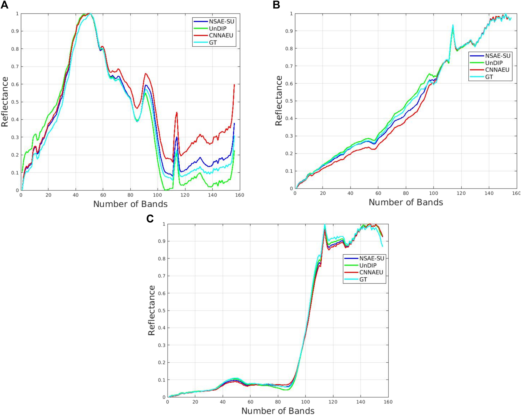
As described in the Experimental analysis section, the Samson dataset possesses three endmembers: water, soil, and road, and the measure used to assess the endmembers’ fidelity is the SAD, as described in the Performance metrics section. Table 4 shows the performance obtained for the baseline algorithms and the NSAE-SU. The NSAE-SU algorithm achieved better performance for the water endmember extraction, obtaining metrics of 0.060 and 0.025 for the soil, and it achieved the best mean SAD. On the other hand, the abundance maps are evaluated using the RMSE metric (Table 5). Figure 6 illustrates the abundance maps for UnDIP, CNNAEU, GT, and NSAE-SU algorithms. In this evaluation, our algorithm outperforms the other baseline algorithms, achieving better results for water 0.091 and soil 0.187.The second benchmark dataset under study is the Jasper Ridge dataset. This dataset consists of four endmembers: water, tree, soil, and road. The GT and the abundances maps are depicted in Figure 8. Table 6 presents the performance of endmember extraction measured by the SAD. Notably, the NSAE-SU method outperforms other algorithms, achieving an SAD of 0.039 for the tree endmember and 0.068 for the road endmember. The water endmember also yields a favorable SAD value of 0.077. In terms of mean SAD, the NSAE-SU method demonstrates superior performance compared to baseline algorithms, with an average SAD of 0.076. Furthermore, the extracted endmembers are illustrated in Figure 7. Regarding the abundance maps, better performance is observed for the water abundance map with an RMSE of 0.1121, and an RMSE of 0.2316 is observed for the soil abundance map (as indicated in Table 7). Figure 8 displays the abundance maps obtained for CNNAEU, UnDIP, NSAE-SU, and the GT.
TABLE 4
| Method/materials | NSAE-SU | UnDIP | CNNAEU | VCA | CAE | MV-NTF |
|---|---|---|---|---|---|---|
| Water | 0.060 | 0.130 | 0.113 | 0.200 | 0.710 | 0.091 |
| Tree | 0.029 | 0.022 | 0.041 | 0.055 | 0.066 | 0.754 |
| Soil | 0.025 | 0.040 | 0.048 | 1.839 | 0.182 | 0.254 |
| Mean SAD | 0.038 | 0.064 | 0.067 | 2.095 | 0.320 | 0.366 |
Comparison between the models UnDIP (Yu et al., 2022), CNNAEU (Yu et al., 2022), VCA (Nascimento and Dias, 2005; Ranasinghe et al., 2020), CAE (Ranasinghe et al., 2020), MV-NTF (Qian et al., 2017; Zheng et al., 2021), and NSAE-SU model for performing the endmember extraction for the Samson dataset using the spectral angle distance metric.
TABLE 5
| Method/materials | NSAE-SU | UnDIP | CNNAEU | VCA | CAE | MV-NTF |
|---|---|---|---|---|---|---|
| Water | 0.091 | 0.426 | 0.202 | 1.111 | 0.279 | 0.503 |
| Tree | 0.172 | 0.252 | 0.172 | 0.245 | 0.181 | 0.438 |
| Soil | 0.187 | 0.267 | 0.198 | 1.284 | 0.284 | 0.441 |
| Mean RMSE | 0.150 | 0.315 | 0.190 | 0.879 | 0.248 | 0.461 |
Comparison between the models: UnDIP (Yu et al., 2022), CNNAEU (Yu et al., 2022), VCA (Nascimento and Dias, 2005; Ranasinghe et al., 2020), CAE (Ranasinghe et al., 2020), MV-NTF (Qian et al., 2017; Zheng et al., 2021), and NSAE-SU model for performing the abundance map estimation for the Samson dataset using the root mean square error metric.
FIGURE 6

Comparison of the abundance maps extracted from the Samson dataset between with the GT or reference maps and the following models: CNNAEU (Palsson et al., 2020), UnDip (Rasti et al., 2022), and NSAE-SU.
TABLE 6
| Method/materials | NSAE-SU | UnDIP | CNNAEU | VCA | CAE | MV-NTF |
|---|---|---|---|---|---|---|
| Water | 0.077 | 0.252 | 0.061 | 0.139 | 0.143 | 0.344 |
| Tree | 0.039 | 0.149 | 0.060 | 0.405 | 0.203 | 0.232 |
| Soil | 0.118 | 0.114 | 0.140 | 1.535 | 0.147 | 0.335 |
| Road | 0.068 | 0.086 | 0.134 | 0.530 | 1.247 | 0.338 |
| Mean SAD | 0.076 | 0.150 | 0.099 | 0.652 | 0.435 | 0.312 |
Comparison between the models UnDIP (Yu et al., 2022), CNNAEU (Yu et al., 2022), VCA (Nascimento and Dias, 2005; Ranasinghe et al., 2020), CAE (Ranasinghe et al., 2020), MV-NTF (Qian et al., 2017; Zheng et al., 2021), and NSAE-SU for performing the endmember extraction for the Jasper Ridge dataset using the spectral angle distance metric.
FIGURE 7

Extracted endmembers for the Jasper Ridge dataset performed by the techniques CNNAE, UnDIP, and NSAE-SU models and compared with the GT. The colors of the endmembers are red—CNNAE, green—UnDIP, blue—NSAE-SU, and cyan—GT. (A) Water spectral signature, (B) road spectral signature, (C) soil spectral signature, and (D) tree spectral signature.
TABLE 7
| Method/materials | NSAE-SU | UnDIP | CNNAEU | VCA | CAE | MV-NTF |
|---|---|---|---|---|---|---|
| Water | 0.112 | 0.201 | 0.183 | 2.212 | 0.133 | 0.298 |
| Tree | 0.172 | 0.160 | 0.199 | 0.380 | 0.201 | 0.387 |
| Soil | 0.232 | 0.132 | 0.294 | 1.754 | 0.193 | 0.396 |
| Road | 0.192 | 0.109 | 0.308 | 0.264 | 0.145 | 0.570 |
| Mean RMSE | 0.177 | 0.150 | 0.246 | 1.152 | 0.168 | 0.413 |
Comparison between the models UnDIP (Yu et al., 2022), CNNAEU (Yu et al., 2022), VCA (Nascimento and Dias, 2005; Ranasinghe et al., 2020), CAE (Ranasinghe et al., 2020), MV-NTF (Qian et al., 2017; Zheng et al., 2021), and the NSAE-SU model for performing the abundance map estimation for the Jasper dataset using the root mean square error metric.
FIGURE 8

Comparison of the abundance maps extracted from the Jasper Ridge database with the GT or reference maps and the following models: CNNAEU (Palsson et al., 2020), UnDip (Rasti et al., 2022), and NSAE-SU.
To verify the robustness of the experimental design and evaluate the NSAE-SU model, the CNNAEU and UnDIP models were executed 10 times each. This was done to facilitate the Wilcoxon statistical analysis on benchmark datasets like Samson and Jasper Ridge, depicted in Figure 9, Figure 10, and Figure 11 respectively, and the extracted endmembers are illustrated for the respective models NSAE-SU, CNNAEU, and UnDIP. Subsequently, the Wilcoxon test is conducted, employing the spectral angle distance metric, on each model’s extracted endmembers. The resulting SAD values from each model are then compared against those from the NSAE-SU model using the Wilcoxon test.
FIGURE 9

The extracted endmembers from 10 runs of the Samson dataset are displayed, for NSAE-SU featured in subfigure (A), CNNAEU in subfigure (B), and UnDIP in subfigure (C).
FIGURE 10

Boxplot analysis illustrating the Wilcoxon results obtained from the comparison of endmember extractions between NSAE-SU and CNNAEU for the Samson dataset. The subfigure (A) displays the water endmember, (B) shows the tree endmember, and (C) shows the soil endmember. Boxplot analysis illustrating the Wilcoxon results obtained from the comparison of endmember extractions between NSAE-SU and UnDIP for the Samson dataset. The subfigure (D) displays the water endmember, (E) shows the tree endmember, and (F) shows the soil endmember.
FIGURE 11

The extracted endmembers from 10 runs of the Jasper dataset are displayed for (A) NSAE-SU, (B) CNNAEU, and (C) UnDIP, respectively.
Figures 10A–C illustrate a boxplot analysis that contrasts NSAE-SU with CNNAEU for the endmembers water, tree, and soil. This analysis reveals statistically significant differences between our algorithm and CNNAEU in the extraction of water and tree endmembers. The NSAE-SU model outperforms by yielding SAD metrics close to 0, indicating high similarity between the endmembers extracted by NSAE-SU. However, for soil, CNNAEU demonstrates superior outcomes. On the other hand, when comparing the NSAE-SU and UnDIP models using the Wilcoxon test, as shown in Figures 10D, E, and 10(F), our algorithm outperforms UnDIP in terms of endmember extraction for water. This improvement is reflected in the better SAD results. Notably, there is a high correlation between the endmembers extracted by NSAE-SU and the ground truth for the Samson dataset. For tree and soil endmembers, UnDIP achieves superior results in the SAD metric.
Figures 12A–D depict boxplot analyses that compare NSAE-SU with CNNAEU for the Jasper Ridge dataset using the Wilcoxon test across the four extracted endmembers. These analyses reveal statistical differences for the water and tree endmembers, with the NSAE-SU model demonstrating a superior performance based on SAD metrics. However, no statistically significant differences were observed for the soil and road endmembers.
FIGURE 12

Boxplot analysis illustrating the Wilcoxon results obtained from the comparison of endmember extractions between NSAE-SU and CNNAEU for the Jasper Ridge dataset. The subfigure (A) displays the water endmember, (B) shows the tree endmember, (C) exhibits the soil endmember, and (D) exhibits the road endmember. In the bottom row, subfigures (E–H) correspondingly exhibit the water, tree, soil, and road endmembers for NSAE-SU vs. UnDIP.
On the contrary, in the comparison between NSAE-SU and UnDIP, as shown in Figures 12E–H, across the four extracted endmembers, this analysis indicates statistical differences for water, tree, and soil. Notably, NSAE-SU exhibits superior performance when compared to UnDIP. However, for the road endmember, UnDIP presents a more favorable SAD metric.
6.2 Endmember extraction and abundance map estimation for the HSI2 Lake Erie hyperspectral image
The NSAE-SU model is employed to extract endmembers, as shown in Figure 13, and computation of fractional abundance maps for the HSI2 image is depicted in Figure 14. This analysis aims to discern the distinct spectral signatures present in the image. The experiment is conducted on the five ROIs selected previously and classified in Manian et al. (2022). The selected ROIs are called the following: red ROI with an area of 25,730 pixels, green ROI with an area of 25,344 pixels, cyan ROI with an area of 19,430, blue ROI with an area of 17,856 pixels, and yellow ROI with an area of 19,296 pixels, as depicted in Figure 4. Once the ROIs are selected, a spectral derivative is used to perform the atmospheric correction, using k = 3, which is defined heuristically.
FIGURE 13

Endmembers extracted from the HSI2 Lake Erie image using the NSAE-SU for each ROI, as follows, (A) red ROI, (B) green ROI, (C) cyan ROI, (D) blue ROI, and (E) yellow ROI.
FIGURE 14

Abundance maps extracted from the selected ROIs for the HSI2 image, where AM-0, AM-1, AM-2, and AM-3 represent the number of the abundance map associated with the endmembers.
The data are then distributed in a patch size of 9, 9, and 170; the number of patches changes due to the difference in the area of the ROIs, as shown in Table 8. Subsequently, each ROI is analyzed, and the abundance maps and endmembers are extracted, as shown in Figure 13.
It is essential to compare the recovered endmembers with baseline spectral signatures to conduct the analysis; for this case study, we propose two comparison methods. The first is a comparison method to analyze the presence of Chl-a spectral signature, which is provided in the paper Ficek et al. (2011) with eight curves that possess the following Chl-a concentrations, respectively, for each curve: 0.020mgL−1, 0.038mgL−1, 0.052mgL−1, 0.112mgL−1, 0.276mgL−1, 0.742mgL−1, 0.966mgL−1, and 1.660mgL−1. Each concentration curve for this analysis will be called Chl-a-1, Chl-a-2, Chl-a-3, Chl-a-4, Chl-a-5, and Chl-a-6, respectively.
TABLE 8
| ROI | Area | Patch size |
|---|---|---|
| Red | 25,730 | (23068, 9, 9, 170) |
| Green | 25,344 | (22680, 9, 9, 170) |
| Cyan | 19,340 | (17125, 9, 9, 170) |
| Blue | 17,856 | (15640, 9, 9, 170) |
| Yellow | 19,296 | (17000, 9, 9, 170) |
Description of the number of patch sizes that are input into the NSAE-SU model. Each ROI is stacked with size 9×9×170 for each area.
The second method involves analyzing the spectral signatures extracted from Liang et al. (2017) of cyanobacteria scum, Nymphoides, Potamogeton, and varying proportions of Chl-a. The concentrations are as follows: suspended solid (SS)—266.2mgL−1, Chl-a—0.0083mgL−1; SS—228.7mgL−1, Chl-a—0.0077mgL−1; SS—127.7mgL−1, Chl-a—0.0034mgL−1; SS—65.9mgL−1, Chl-a—0.0023mgL−1; SS—28.8mgL−1, Chl-a—0.0024mgL−1; SS—21.2mgL−1, and Chl-a—0.0057mgL−1. To distinguish between the labels used for the initial comparison, each concentration curve of Chl-a is assigned a specific identifier: Chl-a-11, Chl-a-22, Chl-a-33, Chl-a-44, Chl-a-55, and Chl-a-66. The SAD metric is employed for the analysis utilizing the reference spectra provided in papers Ficek et al. (2011); Liang et al. (2017), and the endmember estimation is carried out by the NSAE-SU model.
Figure 15A shows the comparison between the reference spectra provided by Ficek et al. (2011) and the spectra obtained for NSAE-SU for the red ROI. The best approximation for the SAD metric is 0.369, which is obtained between the endmember 1 extracted from NSAE-SU and Chl-a-3, which possesses 0.052mgL−1 of the content of Chl-a. Figure 15B analyzes the green ROI, whose best match according to the spectral angle distance is 0.311 between Chl-a-2 and the second endmember extracted from NSAE-SU. The SAD metric obtained for each region of interest using the spectra of Ficek et al. (2011) as ground truth, and the spectra obtained using the NSAE-SU method are summarized in Table 9, for the best endmembers for each ROI. The comparison between the endmembers obtained from NSAE-SU and the ground truth provided by Liang et al. (2017) is evaluated using the SAD metric for each ROI. The results are summarized in Table 10 and depicted in Figures 15C, D. In this context, the term endmembers refers to the spectral signatures extracted from the NSAE-SU model.
FIGURE 15

Comparison between the spectra provided in Ficek et al. (2011), as ground truth, and the spectra extracted by the NSAE-SU model illustrate the best match using the SAD metric for the red and green ROI, respectively. (A) The best match obtained for the red ROI is the Chl-a-3 spectra and the endmember 1 extracted from NSAE-SU. (B) The best match obtained for the green ROI is the Chl-a-2 spectra and the endmember 1 extracted from NSAE-SU. In figures (C) and (D), the provided illustration offers a comparison between the spectra extracted by the NSAE-SU model evaluated using the SAD metric, and the ground truth data from the paper Liang et al. (2017) for the green and cyan regions of interest (ROIs). In (C), the most favorable match for the green ROI aligns with the Chl-a-33 spectra and the endmember 1 extracted from NSAE-SU. (D) for the cyan ROI, the optimal correspondence is observed between the Chl-a-44 spectra and endmember 2 extracted from NSAE-SU.
TABLE 9
| Red ROI | Green ROI | Cyan ROI | Blue ROI | Yellow ROI | |
|---|---|---|---|---|---|
| Chl-a-1 | 0.771 | 0.334 | 0.382 | 0.339 | 0.364 |
| Chl-a-2 | 0.738 | 0.311 | 0.416 | 0.307 | 0.328 |
| Chl-a-3 | 0.369 | 0.352 | 0.754 | 0.463 | 0.456 |
| Chl-a-4 | 0.453 | 0.417 | 0.798 | 0.507 | 0.490 |
| Chl-a-5 | 0.550 | 0.408 | 0.742 | 0.476 | 0.453 |
| Chl-a-6 | 0.605 | 0.567 | 0.896 | 0.629 | 0.601 |
Results for the SAD metric comparison of the spectral signatures of different Chl-a concentrations extracted from Ficek et al. (2011), with the endmembers obtained from NSAE-SU.
TABLE 10
| Red ROI | Green ROI | Cyan ROI | Blue ROI | Yellow ROI | |
|---|---|---|---|---|---|
| Cyanobacterial scums | 0.741 | 0.639 | 0.739 | 0.545 | 0.798 |
| Nymphoides peltata | 0.845 | 0.746 | 0.834 | 0.635 | 0.885 |
| Potamogeton crispus | 0.786 | 0.695 | 0.762 | 0.587 | 0.799 |
| Chl-a-11 | 0.540 | 0.447 | 0.447 | 0.547 | 0.754 |
| Chl-a-22 | 0.654 | 0.617 | 0.640 | 0.733 | 0.857 |
| Chl-a-33 | 0.448 | 0.307 | 0.319 | 0.376 | 0.658 |
| Chl-a-44 | 0.477 | 0.321 | 0.307 | 0.356 | 0.669 |
| Chl-a-55 | 0.616 | 0.549 | 0.547 | 0.650 | 0.822 |
| Chl-a-66 | 0.619 | 0.551 | 0.563 | 0.659 | 0.832 |
Results for the SAD metric comparing the spectral signatures of different Chl-a and macrophytes under different concentrations extracted from Liang et al. (2017), with the endmembers obtained from NSAE-SU.
The concentration of Chl-a-33 compared to endmember 1 demonstrates the best curve fitting for the green ROI, while Chl-a-44 compared to endmember 1 achieves the best curve fitting for the cyan ROI. Additionally, comparing Chl-a-33 to endmember 2 provides the best curve fitting for the yellow ROI, as evaluated using the SAD metric. Figures 15C, D illustrate the optimal curve fitting for the green and cyan ROIs according to the SAD metric. The best concentration of Chl-a for Chl-a-33 is Chl-a 0.0034mgL−1, and for Chl-a-44, it is Chl-a 0.0023mgL−1.
7 Conclusion
An unsupervised deep learning model for endmember extraction and fractional abundance map estimation from the HSI is presented. The NSAE-SU model performs well for the benchmark HSI datasets, such as the Samson and Jasper Ridge datasets, and for the study case of the HSI2 image over Lake Erie. The model is able to identify the endmembers for the water, soil, and road and the abundance maps for water, road, and trees better than the baseline algorithms. Additionally, the spectral signatures extracted using the NSAE-SU model over the Lake Erie HSI is analyzed to determine the presence of Chl-a. The 9 × 9 patch size is determined to be the ideal configuration, and the best hyperparameter settings for the model are listed in Table 3. The models operate at a nominal speed of approximately 3 h and 45 min.
The proposed workflow can be utilized for studying various material compositions within HSIs. Building upon the initial framework, it is feasible to analyze waterbodies and diagnose the condition of coral reefs, as well as assess their degradation. This assessment can be conducted at different time intervals to facilitate change detection by studying distinct spectral signatures present in each image.
Statements
Data availability statement
The original contributions presented in the study are included in the article/Supplementary Material; further inquiries can be directed to the corresponding author.
Author contributions
EA-M, VM, JO, and RT: conceptualization. EA-M, VM, JO, and RF: methodology. EA-M: software, validation, formal analysis, data curation, and writing—original draft preparation. EA-M, VM, JO, and RF: investigation. EA-M and VM: writing—review and editing. VM: project administration and funding acquisition; All authors contributed to the article and approved the submitted version.
Funding
This research was funded by NASA, grant number 80NSSC19M0155. The APC was funded by 80NSSC21M0155. Opinions, findings, conclusions, or recommendations expressed in this material are those of the authors and do not necessarily reflect the views of NASA.
Acknowledgments
We would like to acknowledge the contribution of Mr. Carlos Julian Delgado Munoz to the discussions on the cluster configuration. Additionally, the authors would like to express their gratitude to the reviewers, whose valuable feedback significantly enhanced the quality of the paper.
Conflict of interest
The authors declare that the research is conducted in the absence of any commercial or financial relationships that could be construed as a potential conflict of interest.
Publisher’s note
All claims expressed in this article are solely those of the authors and do not necessarily represent those of their affiliated organizations, or those of the publisher, the editors, and the reviewers. Any product that may be evaluated in this article, or claim that may be made by its manufacturer, is not guaranteed or endorsed by the publisher.
Supplementary material
The Supplementary Material for this article can be found online at: https://www.frontiersin.org/articles/10.3389/feart.2023.1229704/full#supplementary-material
References
1
AhilanA.ManogaranG.RajaC.KadryS.KumarS. N.Agees KumarC.et al (2019). Segmentation by fractional order darwinian particle swarm optimization based multilevel thresholding and improved lossless prediction based compression algorithm for medical images. IEEE Access7, 89570–89580. 10.1109/access.2019.2891632
2
AravindK. R.RajaP.MukeshK.AniirudhR.AshiwinR.SzczepanskiC. (2018). “Disease classification in maize crop using bag of features and multiclass support vector machine,” in 2018 2nd International Conference on Inventive Systems and Control (ICISC) (IEEE), Coimbatore, India, 19-20 January 2018. 10.1109/icisc.2018.8398993
3
AyedM.HanachiR.SellamiA.FarahI. R.MuraM. D. (2022). “A deep learning approach based on morphological profiles for hyperspectral image unmixing,” in 2022 6th International Conference on Advanced Technologies for Signal and Image Processing (ATSIP) (IEEE), Sfax, Tunisia, May 24-27, 2022. 10.1109/atsip55956.2022.9805868
4
BhattJ. S.JoshiM. V. (2020). “Deep learning in hyperspectral unmixing: A review,” in IGARSS 2020 - 2020 IEEE International Geoscience and Remote Sensing Symposium (IEEE), Waikoloa, HI, USA, September 26 - October 2, 2020. 10.1109/igarss39084.2020.9324546
5
ChenS.SunT.YangF.SunH.GuanY. (2018). An improved optimum-path forest clustering algorithm for remote sensing image segmentation. Comput. Geosciences112, 38–46. 10.1016/j.cageo.2017.12.003
6
ChenY.ZhuK.ZhuL.HeX.GhamisiP.BenediktssonJ. A. (2019). Automatic design of convolutional neural network for hyperspectral image classification. IEEE Trans. Geoscience Remote Sens.57, 7048–7066. 10.1109/tgrs.2019.2910603
7
ChongJ. W. R.KhooK. S.ChewK. W.VoD.-V. N.BalakrishnanD.BanatF.et al (2023). Microalgae identification: future of image processing and digital algorithm. Bioresour. Technol.369, 128418. 10.1016/j.biortech.2022.128418
8
ChunhuiZ.BingG.LejunZ.XiaoqingW. (2018). Classification of hyperspectral imagery based on spectral gradient, SVM and spatial random forest. Infrared Phys. Technol.95, 61–69. 10.1016/j.infrared.2018.10.012
9
DasS.ChakrabortyS.RoutrayA.DebA. K. (2019). “Fast linear unmixing of hyperspectral image by slow feature analysis and simplex volume ratio approach,” in IGARSS 2019 - 2019 IEEE International Geoscience and Remote Sensing Symposium (IEEE), Pacifico Yokohama, Japan, 28 July–2. August 2019. 10.1109/igarss.2019.8898127
10
DianR.LiS.FangL.WeiQ. (2019). Multispectral and hyperspectral image fusion with spatial-spectral sparse representation. Inf. Fusion49, 262–270. 10.1016/j.inffus.2018.11.012
11
DingY.GuoY.ChongY.PanS.FengJ. (2021). Global consistent graph convolutional network for hyperspectral image classification. IEEE Trans. Instrum. Meas.70, 1–16. 10.1109/tim.2021.3056750
12
DongY.LiuQ.DuB.ZhangL. (2022). Weighted feature fusion of convolutional neural network and graph attention network for hyperspectral image classification. IEEE Trans. Image Process.31, 1559–1572. 10.1109/tip.2022.3144017
13
DuanP.KangX.LiS.GhamisiP. (2019). Noise-robust hyperspectral image classification via multi-scale total variation. IEEE J. Sel. Top. Appl. Earth Observations Remote Sens.12, 1948–1962. 10.1109/jstars.2019.2915272
14
ErturkA.TaskinG. (2021). “Change detection with manifold embedding for hyperspectral images,” in 2021 11th Workshop on Hyperspectral Imaging and Signal Processing: Evolution in Remote Sensing (WHISPERS) (IEEE), Amsterdam, Netherlands, 24-26 March 2021. 10.1109/whispers52202.2021.9484043
15
FangY.WangY.XuL.ZhuoR.WongA.ClausiD. A. (2022). BCUN: bayesian fully convolutional neural network for hyperspectral spectral unmixing. IEEE Trans. Geoscience Remote Sens.60, 1–14. 10.1109/tgrs.2022.3151004
16
FengJ.ChenJ.LiuL.CaoX.ZhangX.JiaoL.et al (2019). CNN-based multilayer spatial–spectral feature fusion and sample augmentation with local and nonlocal constraints for hyperspectral image classification. IEEE J. Sel. Top. Appl. Earth Observations Remote Sens.12, 1299–1313. 10.1109/jstars.2019.2900705
17
FicekD.ZapadkaT.DeraJ. (2011). Remote sensing reflectance of pomeranian lakes and the baltic.the study was partially financed by MNiSW (ministry of science and higher education) as a research project n n306 066434 in the years 2008–2011. Oceanologia53, 959–970. 10.5697/oc.53-4.959
18
GaoL.HanZ.HongD.ZhangB.ChanussotJ. (2022). CyCU-net: cycle-consistency unmixing network by learning cascaded autoencoders. IEEE Trans. Geoscience Remote Sens.60, 1–14. 10.1109/tgrs.2021.3064958
19
GaoY.PanB.SongX.XuX. (2023). Extended-aggregated strategy for hyperspectral unmixing based on dilated convolution. IEEE Geoscience Remote Sens. Lett.20, 1–5. 10.1109/lgrs.2023.3297577
20
GhoshP.RoyS. K.KoiralaB.RastiB.ScheundersP. (2022). Hyperspectral unmixing using transformer network. IEEE Trans. Geoscience Remote Sens.60, 1–16. 10.1109/tgrs.2022.3196057
21
GoodfellowI.BengioY.CourvilleA. (2016). Deep learning. Massachusetts, United States: MIT Press.
22
GuoH.TianS.HuangJ. J.ZhuX.WangB.ZhangZ. (2022). Performance of deep learning in mapping water quality of lake simcoe with long-term landsat archive. ISPRS J. Photogrammetry Remote Sens.183, 451–469. 10.1016/j.isprsjprs.2021.11.023
23
GuoQ.ZhangJ.ZhongC.ZhangY. (2021). Change detection for hyperspectral images via convolutional sparse analysis and temporal spectral unmixing. IEEE J. Sel. Top. Appl. Earth Observations Remote Sens.14, 4417–4426. 10.1109/jstars.2021.3074538
24
HadiF.YangJ.UllahM.AhmadI.FarooqueG.XiaoL. (2022). DHCAE: deep hybrid convolutional autoencoder approach for robust supervised hyperspectral unmixing. Remote Sens.14, 4433. 10.3390/rs14184433
25
HangR.LiuQ.HongD.GhamisiP. (2019). Cascaded recurrent neural networks for hyperspectral image classification. IEEE Trans. Geoscience Remote Sens.57, 5384–5394. 10.1109/tgrs.2019.2899129
26
HeylenR.ParenteM.GaderP. (2014). A review of nonlinear hyperspectral unmixing methods. IEEE J. Sel. Top. Appl. Earth Observations Remote Sens.7, 1844–1868. 10.1109/jstars.2014.2320576
27
HongD.GaoL.YaoJ.ZhangB.PlazaA.ChanussotJ. (2021). Graph convolutional networks for hyperspectral image classification. IEEE Trans. Geoscience Remote Sens.59, 5966–5978. 10.1109/tgrs.2020.3015157
28
HongD.YokoyaN.ChanussotJ.ZhuX. X. (2019). An augmented linear mixing model to address spectral variability for hyperspectral unmixing. IEEE Trans. Image Process.28, 1923–1938. 10.1109/tip.2018.2878958
29
HouZ.LiW.LiL.TaoR.DuQ. (2022). Hyperspectral change detection based on multiple morphological profiles. IEEE Trans. Geoscience Remote Sens.60, 1–12. 10.1109/tgrs.2021.3090802
30
ImbiribaT.BorsoiR. A.BermudezJ. C. M. (2018). “Generalized linear mixing model accounting for endmember variability,” in 2018 IEEE International Conference on Acoustics, Speech and Signal Processing (ICASSP) (IEEE), Calgary, Alberta, 15-20 April 2018. 10.1109/icassp.2018.8462214
31
JafarzadehH.HasanlouM. (2019). An unsupervised binary and multiple change detection approach for hyperspectral imagery based on spectral unmixing. IEEE J. Sel. Top. Appl. Earth Observations Remote Sens.12, 4888–4906. 10.1109/jstars.2019.2939133
32
LiC.CaiR.YuJ. (2023). An attention-based 3d convolutional autoencoder for few-shot hyperspectral unmixing and classification. Remote Sens.15, 451. 10.3390/rs15020451
33
LiangL.ZhangS.LiJ. (2022). Multiscale DenseNet meets with bi-RNN for hyperspectral image classification. IEEE J. Sel. Top. Appl. Earth Observations Remote Sens.15, 5401–5415. 10.1109/jstars.2022.3187009
34
LiangQ.ZhangY.MaR.LoiselleS.LiJ.HuM. (2017). A modis-based novel method to distinguish surface cyanobacterial scums and aquatic macrophytes in lake taihu. Remote Sens.9. 10.3390/rs9020133
35
LiuH.LiW.XiaX.-G.ZhangM.TaoR. (2021). Superpixelwise collaborative-representation graph embedding for unsupervised dimension reduction in hyperspectral imagery. IEEE J. Sel. Top. Appl. Earth Observations Remote Sens.14, 4684–4698. 10.1109/jstars.2021.3077460
36
LiuS.DuQ.TongX.SamatA.BruzzoneL.BovoloF. (2017). Multiscale morphological compressed change vector analysis for unsupervised multiple change detection. IEEE J. Sel. Top. Appl. Earth Observations Remote Sens.10, 4124–4137. 10.1109/jstars.2017.2712119
37
ManianV.Alfaro-MejíaE.TokarsR. P. (2022). Hyperspectral image labeling and classification using an ensemble semi-supervised machine learning approach. Sensors22. 10.3390/s22041623
38
MengM.LanM.YuJ.WuJ.TaoD. (2020). Constrained discriminative projection learning for image classification. IEEE Trans. Image Process.29, 186–198. 10.1109/tip.2019.2926774
39
MertensS. (2002). Computational complexity for physicists. Comput. Sci. Eng.4, 31–47. 10.1109/5992.998639
40
MiaoY.YangB. (2021). Sparse unmixing for hyperspectral imagery via comprehensive-learning-based particle swarm optimization. IEEE J. Sel. Top. Appl. Earth Observations Remote Sens.14, 9727–9742. 10.1109/jstars.2021.3115177
41
NascimentoJ.DiasJ. (2005). Vertex component analysis: A fast algorithm to unmix hyperspectral data. IEEE Trans. Geoscience Remote Sens.43, 898–910. 10.1109/TGRS.2005.844293
42
OrtizJ. D.AvourisD. M.SchillerS. J.LuvallJ. C.LekkiJ. D.TokarsR. P.et al (2019). Evaluating visible derivative spectroscopy by varimax-rotated, principal component analysis of aerial hyperspectral images from the western basin of lake erie. J. Gt. Lakes. Res.45, 522–535. 10.1016/j.jglr.2019.03.005
43
PalssonB.SveinssonJ. R.UlfarssonM. O. (2019). Spectral-spatial hyperspectral unmixing using multitask learning. IEEE Access7, 148861–148872. 10.1109/access.2019.2944072
44
PalssonB.UlfarssonM. O.SveinssonJ. R. (2020). Convolutional autoencoder for spectral–spatial hyperspectral unmixing. IEEE Trans. Geoscience Remote Sens.59, 535–549. 10.1109/tgrs.2020.2992743
45
ParkJ.BaekJ.KimJ.YouK.KimK. (2022). Deep learning-based algal detection model development considering field application. Water14, 1275. 10.3390/w14081275
46
QiL.ChenZ.GaoF.DongJ.GaoX.DuQ. (2023). Multiview spatial–spectral two-stream network for hyperspectral image unmixing. IEEE Trans. Geoscience Remote Sens.61, 1–16. 10.1109/tgrs.2023.3237556
47
QiL.GaoF.DongJ.GaoX.DuQ. (2022). SSCU-Net: spatial–spectral collaborative unmixing network for hyperspectral images. IEEE Trans. Geoscience Remote Sens.60, 1–15. 10.1109/tgrs.2022.3150970
48
QianY.XiongF.ZengS.ZhouJ.TangY. Y. (2017). Matrix-vector nonnegative tensor factorization for blind unmixing of hyperspectral imagery. IEEE Trans. Geoscience Remote Sens.55, 1776–1792. 10.1109/tgrs.2016.2633279
49
QinA.TanZ.WangR.SunY.YangF.ZhaoY.et al (2023). Distance constraint-based generative adversarial networks for hyperspectral image classification. IEEE Trans. Geoscience Remote Sens.61, 1–16. 10.1109/tgrs.2023.3274778
50
QuY.QiH. (2019). uDAS: an untied denoising autoencoder with sparsity for spectral unmixing. IEEE Trans. Geoscience Remote Sens.57, 1698–1712. 10.1109/tgrs.2018.2868690
51
RanasingheY.HerathS.WeerasooriyaK.EkanayakeM.GodaliyaddaR.EkanayakeP.et al (2020). “Convolutional autoencoder for blind hyperspectral image unmixing,” in 2020 IEEE 15th International Conference on Industrial and Information Systems (ICIIS) (IEEE), Rupnagar, India, 26-28 November 2020. 10.1109/iciis51140.2020.9342727
52
RastiB.KoiralaB.ScheundersP.GhamisiP. (2022). UnDIP: hyperspectral unmixing using deep image prior. IEEE Trans. Geoscience Remote Sens.60, 1–15. 10.1109/tgrs.2021.3067802
53
ShahD.ZaveriT.TrivediY. N.PlazaA. (2020). Entropy-based convex set optimization for spatial–spectral endmember extraction from hyperspectral images. IEEE J. Sel. Top. Appl. Earth Observations Remote Sens.13, 4200–4213. 10.1109/jstars.2020.3008939
54
SheykhmousaM.MahdianpariM.GhanbariH.MohammadimaneshF.GhamisiP.HomayouniS. (2020). Support vector machine versus random forest for remote sensing image classification: A meta-analysis and systematic review. IEEE J. Sel. Top. Appl. Earth Observations Remote Sens.13, 6308–6325. 10.1109/jstars.2020.3026724
55
ShiC.PunC.-M. (2020). Multiscale superpixel-based hyperspectral image classification using recurrent neural networks with stacked autoencoders. IEEE Trans. Multimedia22, 487–501. 10.1109/tmm.2019.2928491
56
ShiC.ZhangT.LiaoD.JinZ.WangL. (2022). Dual hybrid convolutional generative adversarial network for hyperspectral image classification. Int. J. Remote Sens.43, 5452–5479. 10.1080/01431161.2022.2135412
57
SuY.MarinoniA.LiJ.PlazaJ.GambaP. (2018). Stacked nonnegative sparse autoencoders for robust hyperspectral unmixing. IEEE Geoscience Remote Sens. Lett.15, 1427–1431. 10.1109/lgrs.2018.2841400
58
TaneZ.RobertsD.VeraverbekeS.CasasÁ.RamirezC.UstinS. (2018). Evaluating endmember and band selection techniques for multiple endmember spectral mixture analysis using post-fire imaging spectroscopy. Remote Sens.10, 389. 10.3390/rs10030389
59
TongX.YeZ.XuY.GaoS.XieH.DuQ.et al (2019). Image registration with fourier-based image correlation: A comprehensive review of developments and applications. IEEE J. Sel. Top. Appl. Earth Observations Remote Sens.12, 4062–4081. 10.1109/jstars.2019.2937690
60
TsaiF.PhilpotW. (1998). Derivative analysis of hyperspectral data. Remote Sens. Environ.66, 41–51. 10.1016/s0034-4257(98)00032-7
61
TulczyjewL.KawulokM.LongepeN.SauxB. L.NalepaJ. (2022). A multibranch convolutional neural network for hyperspectral unmixing. IEEE Geoscience Remote Sens. Lett.19, 1–5. 10.1109/lgrs.2022.3185449
62
VivoneG. (2023). Multispectral and hyperspectral image fusion in remote sensing: A survey. Inf. Fusion89, 405–417. 10.1016/j.inffus.2022.08.032
63
WagaH.EickenH.LightB.FukamachiY. (2022). A neural network-based method for satellite-based mapping of sediment-laden sea ice in the arctic. Remote Sens. Environ.270, 112861. 10.1016/j.rse.2021.112861
64
WangL.LiuD.WangQ.WangY. (2013). Spectral unmixing model based on least squares support vector machine with unmixing residue constraints. IEEE Geoscience Remote Sens. Lett.10, 1592–1596. 10.1109/lgrs.2013.2262371
65
WinterM. E. (1999). “n-FINDR: an algorithm for fast autonomous spectral end-member determination in hyperspectral data,” in SPIE proceedings. Editors DescourM. R.ShenS. S. (France: SPIE). 10.1117/12.366289
66
WuX.HongD.ChanussotJ. (2023). UIU-Net: U-Net in u-net for infrared small object detection. IEEE Trans. Image Process.32, 364–376. 10.1109/tip.2022.3228497
67
XieW.XieZ.ZhaoF.RenB. (2018). POLSAR image classification via clustering-WAE classification model. IEEE Access6, 40041–40049. 10.1109/access.2018.2852768
68
XuX.SongX.LiT.ShiZ.PanB. (2022). Deep autoencoder for hyperspectral unmixing via global-local smoothing. IEEE Trans. Geoscience Remote Sens.60, 1–16. 10.1109/tgrs.2022.3152782
69
XuY.DuB.ZhangL.CerraD.PatoM.CarmonaE.et al (2019). Advanced multi-sensor optical remote sensing for urban land use and land cover classification: outcome of the 2018 IEEE GRSS data fusion contest. IEEE J. Sel. Top. Appl. Earth Observations Remote Sens.12, 1709–1724. 10.1109/jstars.2019.2911113
70
YangP.TongL.QianB.GaoZ.YuJ.XiaoC. (2021). Hyperspectral image classification with spectral and spatial graph using inductive representation learning network. IEEE J. Sel. Top. Appl. Earth Observations Remote Sens.14, 791–800. 10.1109/jstars.2020.3042959
71
YangX.ChuQ.WangL.YuM. (2022). Water body super-resolution mapping based on multiple endmember spectral mixture analysis and multiscale spatio-temporal dependence. Remote Sens.14, 2050. 10.3390/rs14092050
72
YuY.MaY.MeiX.FanF.HuangJ.LiH. (2022). Multi-stage convolutional autoencoder network for hyperspectral unmixing. Int. J. Appl. Earth Observation Geoinformation113, 102981. 10.1016/j.jag.2022.102981
73
ZabalzaJ.RenJ.ZhengJ.ZhaoH.QingC.YangZ.et al (2016). Novel segmented stacked autoencoder for effective dimensionality reduction and feature extraction in hyperspectral imaging. Neurocomputing185, 1–10. 10.1016/j.neucom.2015.11.044
74
ZhangG.MeiS.XieB.FengY.DuQ. (2022). Spectral variability augmented two-stream network for hyperspectral sparse unmixing. IEEE Geoscience Remote Sens. Lett.19, 1–5. 10.1109/lgrs.2022.3214843
75
ZhengP.SuH.DuQ. (2021). Sparse and low-rank constrained tensor factorization for hyperspectral image unmixing. IEEE J. Sel. Top. Appl. Earth Observations Remote Sens.14, 1754–1767. 10.1109/jstars.2020.3048820
76
ZhongY.WangX.XuY.WangS.JiaT.HuX.et al (2018). Mini-UAV-borne hyperspectral remote sensing: from observation and processing to applications. IEEE Geoscience Remote Sens. Mag.6, 46–62. 10.1109/mgrs.2018.2867592
77
ZhouW.KamataS.-I.WangH.XueX. (2023). Multiscanning-based RNN–transformer for hyperspectral image classification. IEEE Trans. Geoscience Remote Sens.61, 1–19. 10.1109/tgrs.2023.3277014
78
ZhuX.GuoH.HuangJ. J.TianS.ZhangZ. (2023). A hybrid decomposition and machine learning model for forecasting chlorophyll-a and total nitrogen concentration in coastal waters. J. Hydrology619, 129207. 10.1016/j.jhydrol.2023.129207
Summary
Keywords
hyperspectral images, spectral unmixing, endmembers, abundance maps, image processing, deep learning, autoencoder, algal bloom
Citation
Alfaro-Mejía E, Manian V, Ortiz JD and Tokars RP (2023) A blind convolutional deep autoencoder for spectral unmixing of hyperspectral images over waterbodies. Front. Earth Sci. 11:1229704. doi: 10.3389/feart.2023.1229704
Received
05 June 2023
Accepted
04 September 2023
Published
13 October 2023
Volume
11 - 2023
Edited by
Paul Honeine, de traitement de l’information et des systèmes (LITIS), France
Reviewed by
Jiangtao Peng, Hubei University, China
Jakub Nalepa, Silesian University of Technology, Poland
Roozbeh Rajabi, University of Genoa, Italy
Updates
Copyright
© 2023 Alfaro-Mejía, Manian, Ortiz and Tokars.
This is an open-access article distributed under the terms of the Creative Commons Attribution License (CC BY). The use, distribution or reproduction in other forums is permitted, provided the original author(s) and the copyright owner(s) are credited and that the original publication in this journal is cited, in accordance with accepted academic practice. No use, distribution or reproduction is permitted which does not comply with these terms.
*Correspondence: Estefanía Alfaro-Mejía, estefania.alfaro@upr.edu
Disclaimer
All claims expressed in this article are solely those of the authors and do not necessarily represent those of their affiliated organizations, or those of the publisher, the editors and the reviewers. Any product that may be evaluated in this article or claim that may be made by its manufacturer is not guaranteed or endorsed by the publisher.