Multi-frequency wavefield modeling of acoustic VTI wave equation using physics informed neural networks

Incorporating anisotropy is crucial for accurately modeling seismic wave propagation. However, numerical solutions are susceptible to dispersion artifacts, and they often require considerable computational resources. Moreover, their accuracy is dependent on the size of discretization, which is a function of the operating frequency. Physics informed neural networks (PINNs) have demonstrated the potential to tackle long-standing challenges in seismic modeling and inversion, addressing the associated computational bottleneck and numerical dispersion artifacts. Despite progress, PINNs exhibit spectral bias, resulting in a stronger capability to learn low-frequency features over high-frequency ones. This paper proposes the use of a simple fully-connected PINN model, and evaluates its potential to interpolate and extrapolate scattered wavefields that correspond to the acoustic VTI wave equation across multiple frequencies. The issue of spectral bias is tackled by incorporating the Kronecker neural network architecture with composite activation function formed using the inverse tangent (atan), exponential linear unit (elu), locally adaptive sine (l-sin), and locally adaptive cosine (l-cos) activation functions. This allows the construction of an effectively wider neural network with a minimal increase in the number of trainable parameters. The proposed scheme keeps the network size fixed for multiple frequencies and does not require repeated training at each frequency. Numerical results demonstrate the efficacy of the proposed approach in fast and accurate, anisotropic multi-frequency wavefield modeling.

1 Introduction

Although solving the wave equation in time-domain is often computationally efficient and intuitive to our understanding of the wave phenomena, there has been a growing interest in frequency-domain solutions, particularly for applications like migration and full waveform inversion (Pratt, 1999). Frequency-domain wavefield solvers offer reduced dimensionality, but they face computational challenges when inverting the stiffness matrixof the Helmholtz wave equation, especially for large 3-D models or when modeling high-frequency or complex wave physics.

Incorporating anisotropy is crucial for accurately modeling seismic wavefields since a simplistic isotropic assumption of the Earth can yield unsatisfactory outcomes (Brossier et al., 2009), which further exacerbates the imaging challenges. Seismic anisotropy’s influence on wave propagation has been recognized for over 50 years (Postma, 1955; Vander Stoep, 1966). However, it was only in the past 2 decades that it was considered in seismic imaging and inversion due to advancements in computing and data quality. While these improvements make seismic anisotropy more visible, fully accounting for it in the elastic wave equation remains computationally challenging for large models. The transversely isotropic model, introduced byTsvankin (2012), is widely employed to depict the layered structure of the Earth. It assumes that anisotropy is predominantly induced by the gravity-dependent sedimentation process, thereby suggesting a higher likelihood of a vertical axis of symmetry.

To improve the computational efficiency, Alkhalifah (2000) formulated an acoustic wave equation for transversely isotropic media with a vertical symmetry axis (VTI) by utilizing an acoustic dispersion relation that assumes a vertical shear wave velocity of zero (Alkhalifah, 1998). Later, (Zhou et al., 2006), introduced an auxiliary wavefield function and proposed a set of second-order wave equations to simplify the original fourth-order differential equation for VTI media. This new acoustic VTI wave equation (Song and Alkhalifah, 2020), offers enhanced ease of solving and applying waveform inversions compared to the original fourth-order formula. It was noted that solving this equation using the finite-difference method (FD) in the frequency domain is eight times more computationally expensive compared to the isotropic case, placing a significant strain on computing resources (Alkhalifah, 1998).

Accurate and efficient numerical solutions are continuously being sought (Moseley et al., 2020; Dorn and Wu, 2021; Sandhu et al., 2021). Conventional numerical methods have matured over the years, but the progress has been relatively slow. There exists a range of numerical methods, each with its own advantages and suitability for a given problem; however, efforts are continuously in progress to address a multitude of challenges, including but not limited to integrating multi-physics phenomenon, for instance, enhancing the computational efficiency, and/or deriving equivalent simplified mathematical formulations for ease of implementation. Despite their ease of implementation, commonly used conventional methods such as the FD based solvers exhibit reduced accuracy when modeling complex topography. Moreover, FD solvers are susceptible to numerical dispersion artifacts, which result from a slower traveling wave inherent in the solution of the acoustic anisotropic wave equation (Alkhalifah, 2000; Song and Alkhalifah, 2013). While finite-element and spectral-element methods are advantageous over finite-difference schemes, particularly when modeling complex topography, they often require considerable computational resources, and their accuracy is dependent on the quality of meshing (Virieux et al., 2011). Therefore, it is crucial to search for alternative approaches to obtaining wavefield solutions, especially for anisotropic media.

The combination of recent advancements in deep learning theory, substantial improvements in computational power, and the efficient implementation of graph-based algorithms with automatic differentiation (Baydin et al., 2018) has sparked a renewed interest in utilizing neural networks for approximating solutions to partial differential equations (PDEs) (Ovcharenko et al., 2019; Siahkoohi et al., 2019; Moseley et al., 2020). Early contributions exploited supervised learning governed models (Yang and Ma, 2019; Dong et al., 2022; Wang et al., 2023), which often require a large amount of training data, and their reliability is observed to be very dependent on the training set. The recent advent of physics-informed neural network (PINN) (Raissi et al., 2019) has paved new directions in efficiently solving partial differential equations. PINNs offer a meshless framework and restricts the space of admissible solutions by enforcing the physical laws in the loss function instead of pure data-mapping objectives. Integrating structured information into a learning algorithm magnifies the data’s information content, which empowers the algorithm to swiftly converge towards the correct solution and exhibit strong generalization abilities, even when the training dataset is small.

PINNs have demonstrated the potential to tackle long-standing challenges in seismic modeling and inversion (Alkhalifah et al., 2021a; Song and Alkhalifah, 2021; Waheed et al., 2021; Rasht-Behesht et al., 2022). These networks learn to map input spatial locations to corresponding wavefield values that adhere to the Helmholtz equation within an isotropic propagation medium. To overcome the computational bottleneck and numerical dispersion artifacts that arise while modeling wave propagation in an anisotropic medium, an intelligent PINN framework (Song et al., 2021), operating at a single frequency is trained to predict the scattered pressure wavefield instead of the total pressure wavefield. This is because the latter poses convergence issues due to the presence of a point-source singularity. Recently, Wu et al. (2023) also incorporated the scattered field formulation of the acoustic and visco-acoustic wave equation for the treatment of point-source singularity, and identified the challenges posed by non-smooth velocity models in producing accurate wavefields when no boundary conditions are implemented in the loss function. The authors addressed this problem by i) integrating the perfectly matched layers into the loss function, and ii) replacing the affine functions in the argument of the activation function with quadratic functions to improve the estimation of the complex scattered wavefield. It is also demonstrated that pretraining can significantly mitigate the computational cost of PINNs after model alteration.

It is well known that PINN models do well in representing low-frequency features in the wavefield solution while they struggle to approximate high-frequency wavefields. This is due to the well-known “spectral bias” issue (Rahaman et al., 2019). Alkhalifah et al. (2021b) show that by adding frequency as an additional input to the neural network (NN), the same approach could be used to model multi-frequency wavefields simultaneously. This is a significant advantage over conventional numerical solvers, which necessitate the inversion of a separate impedance matrix for each frequency. Although the idea served as a pivotal point, it was noticed that the shallow depths with more energy were predicted better than the deeper parts.

Song and Wang (2023) proposed to use Fourier features in PINN training (Tancik et al., 2020) to simulate multi-frequency wavefields in an isotropic layered model. They demonstrated that Fourier feature PINN could achieve training convergence faster in comparison to the vanilla PINN (which could not resolve multi-frequency wavefields at all); however, its accuracy is shown to be sensitive to the sampling of wavenumbers in the Fourier basis. It is further shown that if the wavenumbers are sampled from a narrower or wider range than the proposed theoretical range, the resolution of the solution at higher frequencies becomes erroneous, causing the training optimization to converge at a higher loss. Another approach by Song and Wang (2022) divides the model into several small pieces, building a mapping between the low and high-frequency wavefields to train a Fourier neural operator. It is then used to predict small pieces of high-frequency wavefields, which are then merged together to generate wavefields for large models. The correlation coefficients between the predictions of the proposed framework and the solutions of the finite difference method yielded discrepancies with an increase in the frequency of interest.

Recently, Waheed (2022) addressed the issue of spectral bias, and encouraged using a Kronecker neural network (KNN) formed by combining different activation functions with sine and cosine activation functions. KNN uses the Kronecker product in the construction of the weight matrices, which allows to construct an effectively wider network than a regular feed-forward neural network with a minor increase in the number of trainable parameters. Numerical results demonstrated that even with a shallow architecture, the proposed approach achieved the desired accuracy for the PINN-based Helmholtz solver compared with using a regular feed-forward NN with a standard activation function. To accurately predict high-frequency wavefields, a recent approach (Huang and Alkhalifah, 2022), called PINNup, was proposed to train a small NN at first to learn the wavefield at a low frequency, and then the neurons are split (producing offspring) to train a larger model for high-frequency wavefield starting with the lower frequency NN parameters. An empirical formula that relates the neuron splitting to the frequency upscaling allows for better accuracy and fast convergence was also presented. Albeit the PINNup approach exhibited superiority compared to the commonly used PINN with the random initialization, the approach requires i) repeated training and utilization of trained weights to initialize the next split-up NN in line, over a range of frequencies until the target frequency is approached; else, a regular large network and training would be required to predict higher frequencies, ii) the model size, as well as the number of training samples from the spatial grid, shall roughly increase by four times as the frequency is doubled, iii) for higher frequencies, the sampling grid has to be much finer than before to generate solutions free of numerical dispersion, and iv) more complex lateral variations in the velocity model might require to split the neurons even more, directly increasing the computational cost.

While PINNs have their own set of challenges, the inherent features make them an efficient and reliable alternative to the aforementioned challenges faced by conventional solvers. Since their introduction, PINNs have been continuously refined and applied to a wide range of aforementioned problems. Taking the growing literature on PINN-based wavefield solvers forward, in this article, we develop a PINN-based algorithm to solve multi-frequency wavefields for the acoustic VTI wave equation. We use a KNN model as developed by Waheed (2022) and explore its ability to interpolate and extrapolate scattered wave fields corresponding to the acoustic VTI wave equation over multiple frequencies. This is the first attempt known to the author at the multi-frequency PINN training for anisotropic media that comes with its own set of challenges. The background wavefield solution used in the scattered acoustic VTI wave equation can be obtained analytically, corresponding to an infinite homogeneous velocity model. The loss function is a sum of the partial differential equation (PDE) misfit and the data misfit (known solutions at two frequencies used while training). The KNN architecture with a composite activation function is incorporated to tackle the spectral bias issue. The proposed scheme keeps the network size fixed for multiple frequencies and does not require repeated training on each frequency.

2 Formulation

2.1 The acoustic VTI wave equation

The anisotropic acoustic wave equation serves as a mathematical model that describes the propagation of waves in an anisotropic medium. The equation is widely used in seismic imaging, reverse-time migration, and full-waveform inversion. When working in the frequency domain and assuming a constant density that is parametrized using the normal move-out (NMO) velocity v_n and the anisotropic parameters δ and η, the acoustic VTI wavefields, in two dimensions (2D), can be solved for using a coupled system of second-order PDEs (Zhou et al., 2006):

$\begin{array}{c}\hfill {\omega }^2{m}_{n}p+\frac{{\partial }^2\left(p+q\right)}{\partial x^2}+\frac{1}{\left(1+2\delta \right)}\frac{{\partial }^{2}p}{\partial z^2}=s,\\ \hfill {\omega }^2{m}_{n}q+2\eta \frac{{\partial }^2\left(p+q\right)}{\partial x^2}=0,\end{array}(1)$

where ω is the angular frequency, $m_n=1/v_n^2$ denotes the NMO squared slowness, p represents the pressure wavefield, q is the auxiliary perturbation wavefield associated with the anisotropic parameter perturbations, s is the source function, and a spatial point inside the domain of interest has coordinates (x, z). Our objective is to solve for the scattered pressure wavefield δ_p = p − p₀, where p₀ is taken to be the background wavefield satisfying the isotropic wave equation:

${\omega }^2{m}_{n0}{p}_0+\frac{{\partial }^2{p}_0}{\partial x^2}+\frac{{\partial }^2{p}_0}{\partial z^2}=s,(2)$

where $m_{n0}{p}_0=1/v_{n0}^2$ represents the squared slowness in an infinite isotropic homogeneous background medium, wherein the anisotropic parameters η₀ = δ₀ = 0. In an isotropic acoustic medium, the auxiliary function q = 0. Assuming a constant velocity and a line source excitation, the isotropic acoustic wave equation admits an analytical solution: $p_0(\mathbf{x})=\frac{\mathrm{i}}{4}{H}_0^{(1)}\left(\omega \sqrt{m_{n0}}\left|\mathbf{x}-{\mathbf{x}}_{\mathbf{s}}\right|\right)$ where $H_0^{(1)}$ is the Hankel function of the first kind and order 0, x = {x, z} represents the spatial coordinates in the Euclidean space, and x_s is the location of the line source. Substituting p = p₀ + δ_p in Eq. 1, we obtain a relation between p₀, δ_p and q which follows:

$s=\frac{{\partial }^2\left(p_0+\delta p+q\right)}{\partial x^2}+\frac{1}{\left(1+2\delta \right)}\frac{{\partial }^2\left(p_0+\delta p\right)}{\partial z^2}+{\omega }^2{m}_n\left(p_0+\delta p\right).(3)$

Defining the squared slowness perturbation $\delta m_n=\frac{1}{v_n^2}-\frac{1}{v_0^2}$, and subtracting 2) from the first equation in system 3), the scattered wavefield δ_p satisfies:

$\begin{array}{cc}\hfill {\omega }^2{m}_n\delta p+\frac{{\partial }^2\left(\delta p+q\right)}{\partial x^2}+\frac{1}{1+2\delta }\frac{{\partial }^2\delta p}{\partial z^2}& =-{\omega }^2\delta m_n{p}_0\hfill \\ \hfill & -\left(\frac{1}{1+2\delta }-1\right)\frac{{\partial }^2{p}_0}{\partial z^2},\hfill \\ \hfill {\omega }^2{m}_{n}q+2\eta \frac{{\partial }^2\left(\delta p+q\right)}{\partial x^2}& =-2\eta \frac{{\partial }^2{p}_0}{\partial x^2}.\hfill \end{array}(4)$

It can be observed that the right-hand side source function is now related to the model perturbation and the background wavefield, acting as a secondary source. This is the Lippmann Schwinger form of the acoustic VTI wave equation (Lippmann and Schwinger, 1950), without any further approximations introduced.

2.2 The PINNs

To solve Eq. 4 using a PINN model, a fully connected deep NN with three inputs corresponding to the spatial coordinates of the solution domain and the range of frequencies {x, z, ω}. There are also four target output values corresponding to the real and imaginary parts of the complex scattered wavefield δ_p (x, z, ω) and auxiliary wavefield q (x, z, ω) corresponding to (4).

PINN-based wavefield computation often requires deep and wide neural networks with standard activation functions, leading to a large computational burden. Instead, the KNN architecture that uses the Kronecker product in the construction of weight matrices is employed here. This enables the creation of a wider network with a minor increase in trainable parameters compared to a regular feed-forward NN, without the need for explicit computation of the Kronecker products. The KNN is instead implemented using a standard feed-forward NN with composite activation functions formed by a combination of inverse tangent (atan), exponential linear unit (elu), locally adaptive sine (l-sin), and locally adaptive cosine (l-cos) activation functions (Waheed, 2022). This allows us to get rid of saturation regions from the output of every layer in the NN and improve the training dynamics. Training the network seeks to minimize the following loss function:

$\begin{array}{ll}\hfill \mathfrak{L}& =\frac{1}{N_t}{\displaystyle \sum _{i=1}^{N_t}}\left({\omega }^2{m}_n^{\left(i\right)}\delta p^{\left(i\right)}+\frac{{\partial }^2\left(\delta p^{\left(i\right)}+q^{\left(i\right)}\right)}{\partial x^2}+{\omega }^2\delta m_n^{\left(i\right)}{p}_0^{\left(i\right)}\right.\hfill \\ \hfill & {\left.+\frac{1}{1+2{\delta }^{\left(i\right)}}\frac{{\partial }^2\delta p^{\left(i\right)}}{\partial z^2}+\left(\frac{1}{1+2{\delta }^{\left(i\right)}}-1\right)\times \frac{{\partial }^2{p}_0^{\left(i\right)}}{\partial z^2}\right)}^2\hfill \\ \hfill & +\frac{1}{N_t}{\displaystyle \sum _{i=1}^{N_t}}{\left({\omega }^2{m}_n^{\left(i\right)}{q}^{\left(i\right)}+2{\eta }^{\left(i\right)}\frac{{\partial }^2\left(\delta p^{\left(i\right)}+q^{\left(i\right)}+p_0^{\left(i\right)}\right)}{\partial x^2}\right)}^2\hfill \\ \hfill & +\frac{1}{N_f}{\displaystyle \sum _{j=1}^{N_f}}\left\{\frac{1}{N_t}{\displaystyle \sum _{i=1}^{N_t}}{\left(\delta p^{\left(i\right)\left(j\right)}-\xi p^{\left(i\right)\left(j\right)}\right)}^2\right\}.\hfill \end{array}(5)$

A few comments about the loss function in Eq. 5 are in order: i) the first two terms represent the mean squared error in approximating the PDE, ii) since it is difficult for PINNs to learn high-frequency wavefields, the KNN predicted wavefields δp are enforced to match the FD based true wavefields ξp at two frequencies (N_f = 2) included in the training process, which range between 3 Hz and 7 Hz. These two frequencies are chosen to be 3 Hz and 4 Hz while training the KNN to extrapolate, and 3 Hz and 7 Hz while training the KNN to interpolate wavefields across all the frequencies. The indices corresponding to these two frequencies from the input data set {x, z, ω} are predetermined such that only these indices contribute to the third term in the loss function.

Here N_t represents the number of random training samples. The anisotropic parameters η, δ, the background wavefield p₀, and the model information, are implicit variables and their ordering must be consistent with the input coordinates. The loss function 5) is initially optimized using the Adam optimizer with a stochastic gradient descent method, and then using the Limited-memory Broyden–Fletcher–Goldfarb–Shanno (LBFGS) algorithm. A full-batch gradient is utilized, with a learning rate of 0.001. Once the KNN is trained, the scattered wavefields are predicted on a regular grid. The PINN model is implemented using the SciANN package (Haghighat and Juanes, 2021)—a high level Tensorflow wrapper for scientific computing.

3 Numerical results

In this section, the proposed idea is tested on a layered velocity model extracted from the left side of the anisotropic Marmousi model and slightly smoothed and shown along with δ and η profiles in Figure 1. A shallow, isotropic water layer is set up on the top of the model, and the source is placed at the surface at 1.25 km. The model is discretized using 101 × 101 cells of length 25m in both the vertical and horizontal directions.

FIGURE 1

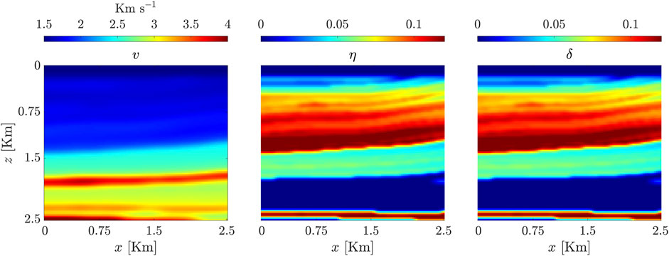
FIGURE 1. The layered velocity model and associated profiles for anisotropic parameters δ and η. The background has a constant velocity of 1.5 km⁻¹.

The background wavefield is computed analytically, considering a homogeneous velocity of 1.5 km s⁻¹. The PINNs are trained for a range of frequencies, with a step size of 1 Hz between 3 Hz and 7 Hz. The proposed PINN comprises four layers with 100 neurons each, where the output of each layer is subject to a composite activation function, wherein atan, elu, l–sin, and l–cos functions are incorporated, Figure 2, with a learnable scaling parameter to avoid the need for problem–specific selection. The network is initially trained for 100,000 epochs using the Adam optimizer, with a learning rate of 0.001, followed by 15,000 epochs of the LBFGS optimizer. This is to break the stagnant training region or when the optimizer gets stuck in local minima. The training loss curve is shown in Figure 3.

FIGURE 2

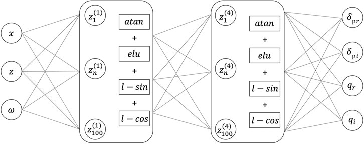
FIGURE 2. The KNN architecture employed in this work.

FIGURE 3

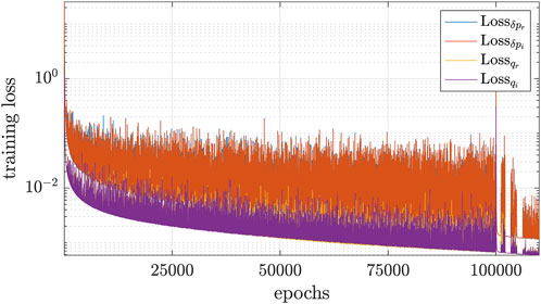
FIGURE 3. Training loss for the proposed network: real and imaginary parts of the data misfit variables, ${\mathrm{L}\mathrm{o}\mathrm{s}\mathrm{s}}_{\delta p_r}$, ${\mathrm{L}\mathrm{o}\mathrm{s}\mathrm{s}}_{\delta p_i}$, ${\mathrm{L}\mathrm{o}\mathrm{s}\mathrm{s}}_{q_r}$, and ${\mathrm{L}\mathrm{o}\mathrm{s}\mathrm{s}}_{q_i}$.

Figure 4 plots the resulting wavefield for interpolation and extrapolation tests. In the first case, 3 Hz and 7 Hz wavefield solutions are provided as training data, while the (4–6) Hz scattered wavefields are learned through the PDE training in the loss function. We observe that the residuals are generally small and we are able to recover the scattered wavefield to a good approximation except for some mild scattering details.

FIGURE 4

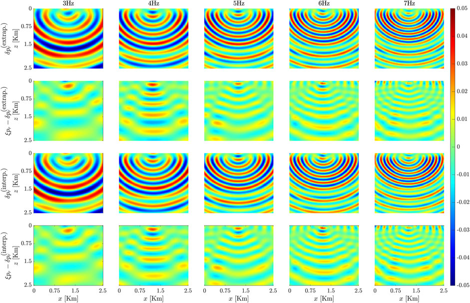
FIGURE 4. Outcomes of testing the interpolation and extrapolation ability of the proposed KNN model. The images corresponds to the real components of the anisotropic wavefields for frequencies ranging from 3Hz to 7 Hz. Firstrow: interpolated scattered wavefields δp_r using the KNN model. Secondrow: Difference between δp_r in the first row and ξp_r i.e., the FD computed wavefields. Thirdrow: extrapolation scattered wavefields δp_r using the KNN model, and Fourthrow: difference between δp_r in the third row and ξp_r i.e., the FD computed wavefields.

However, more importantly, we also show the results in which 3 Hz and 4 Hz wavefields are used as training data while (4–7) Hz wavefields are learned through the PDE term in PINN training. We observe similar accuracy for the extrapolation case as before. This is important because the cost of computing high-frequency wavefields using conventional methods is higher than the lower frequencies. Therefore, one can generate low-frequency solutions using conventional methods and then use PINNs for higher frequencies. This hybrid approach can result in a better accuracy-speed tradeoff.

4 Discussion and conclusion

We addressed the multi-frequency wavefield modeling of the anisotropic acoustic wave equation using a feed-forward NN, where the spectral bias is tackled by incorporating the KNN framework, which allows for constructing an effectively wider NN with a minimal increase in the number of trainable parameters. Numerical tests demonstrate that the proposed approach can successfully interpolate and extrapolate wavefields within a specified frequency range. To solve for even higher frequencies in a computationally tractable manner, the proposed approach can be combined with the frequency scaling and neuron splitting method (Huang and Alkhalifah, 2022). Furthermore, the network can be trained for rapid wavefield computation for any source–receiver pair in the computational domain.

Through extrapolation tests, we show that by feeding wavefield solutions from low frequencies, the high-frequency wavefields can be accurately predicted, harnessing the PDE in the loss function. Based on our experience and the existing PINN literature, relying solely on the PDE for the training of wavefield can be computationally intractable. Therefore, we condition the PINN model to converge faster to the correct solution by providing wavefield solutions for low frequencies. These ideas are also validated in a very recent contribution by Wu et al. (2023). Such an approach is likely to yield the best accuracy-speed tradeoff for PINN-based modeling schemes that are often criticized for their lack of computational efficiency. To further enhance the accuracy of our approach, we envision integrating ideas from the work of Wu et al. (2023). This integration would provide an exciting avenue for future research and development.

In the context of our investigation, an often cited challenge for PINNs based solvers is their potential convergence to a trivial solution. This could render the solution inaccurate even though the loss curve may show convergence. However, our approach mitigates this issue by incorporating the solution for low frequencies as data in the training of the PINN. This inclusion of low-frequency data supplies the network with additional, rich contextual information, which averts the risk of the solver gravitating towards a trivial solution. Therefore, our method not only enhances the robustness of the PINN model but also ensures its viability in dealing with complex problem landscapes.

Data availability statement

The original contributions presented in the study are included in the article/supplementary material, further inquiries can be directed to the corresponding author.

Author contributions

AS: Conceptualization, Methodology, Software. UW: Conceptualization, Supervision, Reviewing and Editing. CS: Reviewing and Editing. OD: Reviewing and Editing. PS: Reviewing and Editing. All authors contributed to the article and approved the submitted version.

Funding

We acknowledge the generous support by the College of Petroleum Engineering and Geosciences (CPG) at King Fahd University of Petroleum and Minerals (KFUPM) through the Competitive Research Grant CPG 21103.

Conflict of interest

The authors declare that the research was conducted in the absence of any commercial or financial relationships that could be construed as a potential conflict of interest.

The reviewer XD declared a shared affiliation with the author CS to the handling editor at the time of review.

Publisher’s note

All claims expressed in this article are solely those of the authors and do not necessarily represent those of their affiliated organizations, or those of the publisher, the editors and the reviewers. Any product that may be evaluated in this article, or claim that may be made by its manufacturer, is not guaranteed or endorsed by the publisher.

References

Alkhalifah, T., Song, C., bin Waheed, U., and Hao, Q. (2021a). Wavefield solutions from machine learned functions constrained by the helmholtz equation. Artif. Intell. Geosciences 2, 11–19. doi:10.1016/j.aiig.2021.08.002

CrossRef Full Text | Google Scholar

Alkhalifah, T. (1998). Acoustic approximations for processing in transversely isotropic media. Geophysics 63, 623–631. doi:10.1190/1.1444361

CrossRef Full Text | Google Scholar

Alkhalifah, T. (2000). An acoustic wave equation for anisotropic media. Geophysics 65, 1239–1250. doi:10.1190/1.1444815

CrossRef Full Text | Google Scholar

Alkhalifah, T., Song, C., and Huang, X. (2021b). “High-dimensional wavefield solutions based on neural network functions,” in First international meeting for applied geoscience and energy (Houston, Texas, United States: Society of Exploration Geophysicists), 2440–2444.

CrossRef Full Text | Google Scholar

Baydin, A. G., Pearlmutter, B. A., Radul, A. A., and Siskind, J. M. (2018). Automatic differentiation in machine learning: A survey. J. Marchine Learn. Res. 18, 1–43.

Google Scholar

Brossier, R., Operto, S., and Virieux, J. “2d elastic frequency-domain full-waveform inversion for imaging complex onshore structures,” in Proceedings of the 71st EAGE Conference and Exhibition incorporating SPE EUROPEC 2009, Amsterdam, Netherlands, June 2009.

Google Scholar

Dong, X., Lin, J., Lu, S., Huang, X., Wang, H., and Li, Y. (2022). Seismic shot gather denoising by using a supervised-deep-learning method with weak dependence on real noise data: A solution to the lack of real noise data. Surv. Geophys. 43, 1363–1394. doi:10.1007/s10712-022-09702-7

CrossRef Full Text | Google Scholar

Dorn, O., and Wu, Y. (2021). Shape reconstruction in seismic full waveform inversion using a level set approach and time reversal. J. Comput. Phys. 427, 110059. doi:10.1016/j.jcp.2020.110059

CrossRef Full Text | Google Scholar

Haghighat, E., and Juanes, R. (2021). Sciann: A keras/tensorflow wrapper for scientific computations and physics-informed deep learning using artificial neural networks. Comput. Methods Appl. Mech. Eng. 373, 113552. doi:10.1016/j.cma.2020.113552

CrossRef Full Text | Google Scholar

Huang, X., and Alkhalifah, T. (2022). Pinnup: robust neural network wavefield solutions using frequency upscaling and neuron splitting. J. Geophys. Res. Solid Earth 127, e2021JB023703. doi:10.1029/2021jb023703

CrossRef Full Text | Google Scholar

Lippmann, B. A., and Schwinger, J. (1950). Variational principles for scattering processes. i. Phys. Rev. 79, 469–480. doi:10.1103/physrev.79.469

CrossRef Full Text | Google Scholar

Moseley, B., Nissen-Meyer, T., and Markham, A. (2020). Deep learning for fast simulation of seismic waves in complex media. Solid earth. 11, 1527–1549. doi:10.5194/se-11-1527-2020

CrossRef Full Text | Google Scholar

Ovcharenko, O., Kazei, V., Kalita, M., Peter, D., and Alkhalifah, T. (2019). Deep learning for low-frequency extrapolation from multioffset seismic data. Geophysics 84, R989–R1001. doi:10.1190/geo2018-0884.1

CrossRef Full Text | Google Scholar

Postma, G. (1955). Wave propagation in a stratified medium. Geophysics 20, 780–806. doi:10.1190/1.1438187

CrossRef Full Text | Google Scholar

Pratt, R. G. (1999). Seismic waveform inversion in the frequency domain, part 1: theory and verification in a physical scale model. Geophysics 64, 888–901. doi:10.1190/1.1444597

CrossRef Full Text | Google Scholar

Rahaman, N., Baratin, A., Arpit, D., Draxler, F., Lin, M., Hamprecht, F., et al. (2019). On the spectral bias of neural networks. https://arxiv.org/abs/1806.08734.

Google Scholar

Raissi, M., Perdikaris, P., and Karniadakis, G. E. (2019). Physics-informed neural networks: A deep learning framework for solving forward and inverse problems involving nonlinear partial differential equations. J. Comput. Phys. 378, 686–707. doi:10.1016/j.jcp.2018.10.045

CrossRef Full Text | Google Scholar

Rasht-Behesht, M., Huber, C., Shukla, K., and Karniadakis, G. E. (2022). Physics-informed neural networks (pinns) for wave propagation and full waveform inversions. J. Geophys. Res. Solid Earth 127, e2021JB023120. doi:10.1029/2021jb023120

CrossRef Full Text | Google Scholar

Sandhu, A. I., Shaukat, S. A., Desmal, A., and Bagci, H. (2021). Ann-assisted cosamp algorithm for linear electromagnetic imaging of spatially sparse domains. IEEE Trans. Antennas Propag. 69, 6093–6098. doi:10.1109/tap.2021.3060547

CrossRef Full Text | Google Scholar

Siahkoohi, A., Louboutin, M., and Herrmann, F. J. (2019). Neural network augmented wave-equation simulation. https://arxiv.org/abs/1910.00925.

Google Scholar

Song, C., and Alkhalifah, T. (2020). An efficient wavefield inversion for transversely isotropic media with a vertical axis of symmetry. Geophysics 85, R195–R206. doi:10.1190/geo2019-0039.1

CrossRef Full Text | Google Scholar

Song, C., and Alkhalifah, T. A. (2021). Wavefield reconstruction inversion via physics-informed neural networks. IEEE Trans. Geoscience Remote Sens. 60, 1–12. doi:10.1109/tgrs.2021.3123122

CrossRef Full Text | Google Scholar

Song, C., Alkhalifah, T., and Waheed, U. B. (2021). Solving the frequency-domain acoustic vti wave equation using physics-informed neural networks. Geophys. J. Int. 225, 846–859. doi:10.1093/gji/ggab010

CrossRef Full Text | Google Scholar

Song, C., and Wang, Y. (2022). High-frequency wavefield extrapolation using the Fourier neural operator. J. Geophys. Eng. 19, 269–282. doi:10.1093/jge/gxac016

CrossRef Full Text | Google Scholar

Song, C., and Wang, Y. (2023). Simulating seismic multifrequency wavefields with the Fourier feature physics-informed neural network. Geophys. J. Int. 232, 1503–1514. doi:10.1093/gji/ggac399

CrossRef Full Text | Google Scholar

Song, X., and Alkhalifah, T. (2013). Modeling of pseudoacoustic p-waves in orthorhombic media with a low-rank approximation. Geophysics 78, C33–C40. doi:10.1190/geo2012-0144.1

CrossRef Full Text | Google Scholar

Tancik, M., Srinivasan, P., Mildenhall, B., Fridovich-Keil, S., Raghavan, N., Singhal, U., et al. (2020). Fourier features let networks learn high frequency functions in low dimensional domains. Adv. Neural Inf. Process. Syst. 33, 7537–7547.

Google Scholar

Tsvankin, I. (2012). Seismic signatures and analysis of reflection data in anisotropic media. Houston, Texas, United States: Society of Exploration Geophysicists.

Google Scholar

Vander Stoep, D. (1966). Velocity anisotropy measurements in wells. Geophysics 31, 900–916. doi:10.1190/1.1439822

CrossRef Full Text | Google Scholar

Virieux, J., Calandra, H., and Plessix, R.-É. (2011). A review of the spectral, pseudo-spectral, finite-difference and finite-element modelling techniques for geophysical imaging. Geophys. Prospect. 59, 794–813. doi:10.1111/j.1365-2478.2011.00967.x

CrossRef Full Text | Google Scholar

Waheed, U. B., Haghighat, E., Alkhalifah, T., Song, C., and Hao, Q. (2021). PINNeik: eikonal solution using physics-informed neural networks. Comput. Geosciences 155, 104833. doi:10.1016/j.cageo.2021.104833

CrossRef Full Text | Google Scholar

Waheed, U. B. (2022). Kronecker neural networks overcome spectral bias for pinn-based wavefield computation. IEEE Geoscience Remote Sens. Lett. 19, 1–5. doi:10.1109/lgrs.2022.3209901

CrossRef Full Text | Google Scholar

Wang, H., Lin, J., Dong, X., Lu, S., Li, Y., and Yang, B. (2023). Seismic velocity inversion transformer. Geophysics 88, R513–R533. doi:10.1190/geo2022-0283.1

CrossRef Full Text | Google Scholar

Wu, Y., Aghamiry, H. S., Operto, S., and Ma, J. (2023). Helmholtz-equation solution in nonsmooth media by a physics-informed neural network incorporating quadratic terms and a perfectly matching layer condition. Geophysics 88, T185–T202. doi:10.1190/geo2022-0479.1

CrossRef Full Text | Google Scholar

Yang, F., and Ma, J. (2019). Deep-learning inversion: A next-generation seismic velocity model building method. Geophysics 84, R583–R599. doi:10.1190/geo2018-0249.1

CrossRef Full Text | Google Scholar

Zhou, H., Zhang, G., and Bloor, R. “An anisotropic acoustic wave equation for vti media,” in Proceedings of the 68th EAGE Conference and Exhibition incorporating SPE EUROPEC 2006, Vienna, Austria, June 2006.

Google Scholar