 Giovanni Messuti1,2*
 Silvia Scarpetta1,2
 Ortensia Amoroso1*
 Ferdinando Napolitano1
 Mariarosaria Falanga3
 Paolo Capuano1
- 1Department of Physics “E.R. Caianiello”, University of Salerno, Fisciano, Italy
- 2Section of Naples, National Institute for Nuclear Physics (INFN), Naples, Italy
- 3Department of Information and Electrical Engineering and Applied Mathematics (DIEM), University of Salerno, Fisciano, Italy
First-motion polarity determination is essential for deriving volcanic and tectonic earthquakes’ focal mechanisms, which provide crucial information about fault structures and stress fields. Manual procedures for polarity determination are time-consuming and prone to human error, leading to inaccurate results. Automated algorithms can overcome these limitations, but accurately identifying first-motion polarity is challenging. In this study, we present the Convolutional First Motion (CFM) neural network, a label-noise robust strategy based on a Convolutional Neural Network, to automatically identify first-motion polarities of seismic records. CFM is trained on a large dataset of more than 140,000 waveforms and achieves a high accuracy of 97.4% and 96.3% on two independent test sets. We also demonstrate CFM’s ability to correct mislabeled waveforms in 92% of cases, even when they belong to the training set. Our findings highlight the effectiveness of deep learning approaches for first-motion polarity determination and suggest the potential for combining CFM with other deep learning techniques in volcano seismology.
1 Introduction
In the field of Earth sciences, the study of seismic waves generated by earthquakes occupies an important role since it allows us to retrieve the main features of both the propagation medium and the seismic source. As for the seismic source, the attention is mainly devoted to estimating the geometric and kinematic parameters, including the location, magnitude, fault dimension and focal mechanisms. Focal mechanisms are crucial to characterize the seismogenic fault structures and the stress field of a region, from local to nationwide scale, in tectonic (Vavryčuk, 2014; Napolitano et al., 2021a; Uchide et al., 2022), and volcanic areas (Roman et al., 2006; Judson et al., 2018; La Rocca and Galluzzo, 2019; Aoki, 2022; Zhan et al., 2022).
The focal mechanisms can be computed using P-wave first-motion polarity (e.g., FPFIT; Reasenberg, 1985; Snoke et al., 2003; Hardebeck and Shearer, 2002), the waveform information (e.g., Zhao and Helmberger, 1994) or both (Weber, 2018). P-wave polarity is also used as an additional constraint in the moment-tensor inversion (e.g., in volcanic settings, Dahm and Brandsdottir, 1997; Miller et al., 1998; Pesicek et al., 2012; Alvizuri and Tape, 2016) and full waveform inversion (e.g., for explosion Chiang et al., 2014; Ford et al., 2009). Determining first-motion polarities by manual procedures, mostly done for larger events, is time-consuming, susceptible to human error and can result in different outcomes depending on the expert analyst. In addition, a proper identification of the first-motion polarity can be difficult when dealing with small magnitude earthquakes. This may be due to the unfavorable signal-to-noise ratio. An enhanced method of identifying first-motion polarities will allow us to resolve the focal mechanism of smaller magnitude events, thereby improving our ability to characterize and interpret seismogenic areas. Automated procedures (e.g., Chen and Holland, 2016; Pugh et al., 2016) can avoid drawbacks, such as time consumption and ensure reproducibility. Despite this, identifying first-motion polarity is not a straightforward classification task that can be easily expressed using mathematical procedures. Consequently, the effectiveness of the automated algorithms (not based on machine learning) relies on a limited number of parameters, which require intensive human involvement to fine-tune, and may result in worse performance compared to human analysis (Ross et al., 2018).
Deep learning offers a notable advantage in that prior knowledge of the observed phenomena is not a prerequisite for model development. This is attributed to the capability of Deep Neural Networks (DNNs) to autonomously extract significant features from raw data, eliminating the need for a mathematical representation of the problem. Moreover, when confronted with extensive datasets, deep learning has proved to be a suitable and highly effective methodology to be employed. Hence, the vast amount of seismological data represents an excellent opportunity for the application of DNNs, making deep learning an ideal choice for our purposes. Recent studies demonstrated the possibility of developing effective and competitive applications of DNNs in the study of seismic waves generated by earthquakes, volcanic eruptions, explosions, along with other sources (Mousavi and Beroza, 2022). DNNs have been used for events detection and location (Perol et al., 2018), arrival times picking (Ross et al., 2018; Zhu and Beroza, 2019), data denoising (Richardson and Feller, 2019), classification of volcano-seismic events (López-Pérez et al., 2020), construction of suitable ontologies (Falanga et al., 2022), discrimination of explosive and tectonic sources (Linville et al., 2019; Kong et al., 2022), waveform recognition both focusing on transients and continuous background acquisition (Rincon-Yanez et al., 2022) and for ground motion prediction equations (Prezioso et al., 2022).
Several studies have demonstrated the significant applicability of Convolutional Neural Networks (LeCun et al., 2015) in determining the first-motion polarity. CNNs use convolutional layers to extract spatial patterns from a multi-dimensional input array or matrix-like data. By applying multiple filters with adjustable weights through a process known as convolution, these filters extract relevant features through their scanning process. Stacking multiple convolutional layers allows the network to automatically learn and identify relevant abstract features useful for the task. The ability of CNNs to capture complex spatial relationships has made them particularly effective in a wide range of image and signal processing tasks, including the determination of first-motion polarity. One of the earliest studies in this field, conducted by Ross et al. (2018), involved training a simple CNN on 18.2 million seismograms from the Southern California Seismic Network (SCSN) catalog, achieving a precision in determining polarities of 95%. Hara et al. (2019) established a lower limit on the number of waveforms required for a satisfactory level of performance during training. The same authors explored the possibility of using a CNN to predict waveforms deriving from events located in regions different from those where data used for the training set have been collected. Uchide (2020) derived focal mechanisms and important information about the stress field in Japan exploiting the first-motion polarities determined by using a CNN-based technique. Li et al. (2023) utilized the CNN by Zhao et al. (2023) to develop an automatic workflow for focal mechanism inversion.
In this work, we present the Convolutional First Motion (CFM) neural network, a label-noise robust strategy based on a CNN to automatically identify first-motion polarities of seismic waves. We take advantage of the regularization effects of dropout layers and the implicit regularization properties of Stochastic Gradient Descent (SGD), when used in combination with early stopping, to handle a percentage of mislabelling (often known as noisy labels). CFM is trained on more than 140,000 waveforms derived from INSTANCE dataset (Michelini et al., 2021), and tested both on 8,983 waveforms belonging to different events of the same dataset and on 4,072 waveforms collected from Napolitano et al. (2021b). We found that when CFM is applied to mislabeled waveforms, which we identified through a data visualization procedure, it corrects them in 92% of the cases, even when they belong to the training set. CFM showed high accuracy levels (i.e., 97.4% and 96.3%) when tested on two independent test sets, high reliability and great generalization ability. The approach shown in our study reveals that an appropriate augmentation procedure can make the network able to deal with uncertainty in arrival times, which increases the potential for using CFM in combination with automatic deep learning techniques for phase picking. Such methodology is expected to have a strong impact on any problem related to the source modeling of tectonic and volcanic quakes, whose construction is founded on the best picking and phase recognition.
2 Data
We collected the seismic waveforms included in the INSTANCE dataset (Michelini et al., 2021) and used them to train the neural network and to evaluate its performance. The dataset, specifically compiled to apply machine learning techniques, comprises 1,159,249 waveforms originating from different sources (natural and anthropogenic earthquakes, volcanic eruptions, landslides along with other sources). The waveforms were registered by both velocimeters (HH, EH channels) and accelerometers (HN channel) seismometers belonging to 19 seismic networks operated and managed by several Italian institutions. The dataset includes 54,000 earthquakes that occurred between January 2005 and January 2020 in Italy and surrounding regions, with magnitude ranging from 0.0 to 6.5 (see Michelini et al., 2021 for further details). Each datum consists of a 120 s time window. Each waveform is associated with upward, downward, or undefined polarity. We excluded all those events with undefined polarity. In addition, selecting only the vertical component of velocimeters data, we achieved 161,198 seismic traces of which 103,530 showed upward polarity and 57,668 downward polarity. We will refer to these waveforms as dataset A (Figure 1A). We split this dataset into three subsets, respectively used as.
• Training set: 141,972 waveforms (88.0% of the total data) corresponding to 23,878 events shown as red circles in Figure 1A;
• Validation set: 10,243 waveforms (6.4% of the total data) corresponding to 2,275 events shown as orange circles in Figure 1A;
• Testing set: 8,983 waveforms (5.6% of the total data) corresponding to 2,398 events shown as blue circles in Figure 1A.
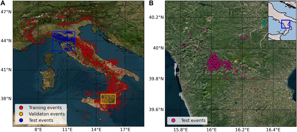
FIGURE 1. Localization of seismic events, shown with circles along the Italian peninsula. (A) The 28,551 events considered in dataset A (derived from the INSTANCE dataset). Waveforms belonging to events displayed by red circles are used as training data. The orange and blue boxes respectively contain events used to derive validation and test waveforms data. (B) The 842 events present in dataset B (derived from Napolitano et al., 2021b), located in Southern Italy, whose waveforms are used as a second test set.
The spatial selection was made to avoid correlations between waveforms in the different sets, following the approach proposed by Uchide (2020). It is noteworthy that the validation set comprises earthquakes from the Etna volcano region (orange box in Figure 1A).
Then, we collected the 870 earthquakes (ML 1.8–5.0), recorded during the 2010–2014 Pollino (Southern Italy) seismic sequence (Figure 1B) by three seismic networks (Istituto Nazionale di Geofisica e Vulcanologia (INGV), Università della Calabria (UniCal) and Deutsche GeoForschungsZentrum (GFZ)) (Passarelli et al., 2012; Margheriti et al., 2013) and located in the new 3D velocity model by Napolitano et al. (2021b). From these events, we selected the vertical components of the waveforms sampled at 100 Hz, registered by velocimeters and with clear P-wave polarity. We refer to this dataset as dataset B. It comprises 4,072 manually picked waveforms derived from 824 out of the original 870 events collected. We used dataset B as a second test set to evaluate the performance of the neural network on data from a specific Italian tectonic setting. To avoid any possible overlapping between dataset A and dataset B, we removed the 821 common waveforms in the former dataset.
In addition, we used seismic traces from the Southern California Seismic Network (Ross et al., 2018) and western Japan region (Hara et al., 2019) to evaluate the network’s generalization ability on waveforms from completely different regions. For this purpose, we selected the 863,151 waveforms belonging to the 273,882 earthquakes registered at 682 stations from the SCSN dataset. This constitutes the part of the test set with definite polarity used in Ross et al. (2018), whose magnitudes lie in the range [−1.0,7.2]. Similarly, we used 3,930 waveforms (ML -1.3–6.2) constituting a part of the test set sampled at 100 Hz provided to us by Hara et al. (2019). The waveforms from the western Japan region were registered by stations operated by the National Research Institute for Earth Science and Disaster Prevention (NIED), the National Institute of Advanced Industrial Science and Technology (AIST), the Japan Meteorological Agency (JMA), and Kyoto University (Hara et al., 2019).
3 Methods
3.1 Data visualization with SOM and label noise
Before training the network on part of dataset A, the preliminary step of our analysis has been the implementation of a data visualization technique to investigate the waveforms. To this end, we applied the Self Organizing Maps (SOM, Kohonen, T., 2013). This unsupervised machine learning technique is highly efficient in reducing the dimensionality of large datasets, by leveraging the similarities between the data, to cluster and visualize them in a low-dimensional grid, while preserving their topological structure. In order to focus the SOM on the features of our interest, the map was given a representation of the data in feature space. We normalized the traces to unit variance and we focused our attention on time windows of 0.26 s (26 samples), which include the 0.20 s preceding the P-arrivals and the 0.05 s after. We used 5 samples after the arrival, as they were enough to capture the entire first oscillation of the seismic wave in the case of higher frequency earthquakes, and enough to point out the trend of the oscillation in the case of lower frequency earthquakes. A lower value was not sufficient to capture the trend of oscillations in low-frequency events, whereas with higher values we observed that the analysis also focused on the second oscillations. We employed 20 samples before the arrival as they constituted the minimum number required to capture the essential characteristics of the noise trend in each scenario. Features provided to the SOM were extracted either by the Principal Component Analysis (Bishop and Nasrabadi, 2006), to which the normalized 0.26-seconds-long time windows were provided, and by evaluating averages of 0.16-seconds-long moving temporal windows. The first average was calculated over the time window starting from 0.19 s before the P-arrival, and the subsequent 9 averages were calculated on shifted windows, moving forward by 0.01 s each (1 sample), with the last time window covering the last 0.16 s (from 0.10 s before the arrival to 0.05 s after). In total, we gave the SOM 16 features, namely, the first 6 principal components and 10 moving averages. We chose to consider the principal components up to the sixth because it was a fair trade-off between the number of dimensions taken into account and the explained variance. By using six components, we were able to achieve a 95% explained variance.
In our analysis, the map nodes were organized in a two-dimensional hexagonal 8 × 8 grid (Supplementary Figure S1B gives a representation of the grid). After the SOM training stage, we displayed the waveforms’ clusters on the map of nodes. Each single node represents a cluster that contains all those data whose distance in input space is smaller than the distance to all other nodes. Supplementary Figure S1A,S2A,S3A show the mean value of the waveforms contained in each node and one-fifth of the waveforms falling in each of them, respectively using the total, upward, and downward first-motion polarity. The number of waveforms in each cluster is represented by the size of the hexagons in Supplementary Figure S1B,S2B,S3B. We observe that the map places most of the waveform with downward polarity on the left side of the grid (Supplementary Figure S3B), especially in the upper part, while the waveforms with upward polarities are mostly placed on the right side of the grid (Supplementary Figure S2B), with the more populated nodes situated in the lower part. The net separation between the two parts provides a strong indication that, generally, the polarities are resolved in an unambiguous way. Nevertheless, a problem often encountered is that the polarities can be mistakenly labeled. To overcome such difficulty, we investigated the SOM results in more detail.
Figure 2 shows in each cell the weighted percentage of traces with upward polarities contained in it. Since the number of downward polarities is smaller than the upward one in dataset A, a weighted percentage is required for a robust analysis. Specifically, the value
where
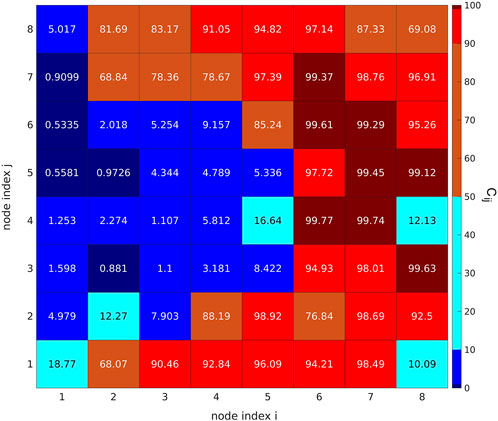
FIGURE 2. Heatmap relative to SOM nodes, showing the weighted percentages
In fact, we manually checked that at least 100 of the 123 down-labeled traces, which fell in nodes with a weighted percentage of up-labeled data above 99%, had indeed an upward polarity. Analogously, at least 237 of the 336 up-labeled traces, located in nodes with more than 99% down-populated data, were clear waveforms with negative polarity. The remaining traces were mostly unclear waveforms, where extracting polarity information was a challenging task also for a human analyst. We do not exclude the presence of other mislabeled data (respect to the 337 found by the SOM visualization). A visual inspection of 1,000 randomly selected waveforms highlighted that approximately 8% of waveforms are affected by some problems, such as noisy arrival times or not reliable polarity information.
This level of noise is very common in real-world datasets, especially in the case of such large ones, where the ratio of corrupted labels can cover, in some cases, up to 40% of the entire dataset (Song et al., 2022). Although it may appear to have drastic consequences to use problematic data to train a classifier, numerous studies have demonstrated that, with appropriate precautions and depending on the nature of the encountered noise, deep learning can exhibit remarkable robustness (Rolnick et al., 2017; Drory et al., 2018). Furthermore, other works highlight that noise can also be useful to better generalize (Damian et al., 2021).
Subsequent investigations revealed that attempting to clean our dataset yielded no significant benefits. Specifically, a second SOM visualization technique, similar to the one previously described, has been applied. This analysis aimed to analyze upward and downward polarity waveforms separately and enabled us to remove from dataset A approximately 10,000 waveforms. We excluded all the waveforms that fell within SOM nodes where we determined the majority of the data to be ambiguous or where extracting polarity information was very challenging. These waveforms comprised elements from the training, validation, and test sets. Supplementary Figure S4 shows some of the excluded nodes. In Supplementary Table S1, we compare the performance of the network trained on the original training set with the network trained on the cleaned training set, presenting the performance on both the cleaned test set and the original test set. Notably, we observed no significant differences in the performance of the two networks, when tested on the same test-set. Therefore, despite the presence of mislabelling in our dataset, we have chosen not to exclude any waveform, but rather, we aimed to design a network that can effectively handle and mitigate the effects of label noise, without the need for a preliminary selection of data points, which can result in information loss.
3.2 CFM architecture and preprocessing stage
The CFM network exclusively utilizes the vertical component of waveforms that have been sampled at a frequency of 100 Hz whose polarity information is available. To ensure consistency of the input data, all waveforms are subjected to a standardized preprocessing stage. Specifically, we subtracted to each waveform the mean value of the noise, from 200 samples (2.0 s) before the corresponding P arrival time to 5 samples before (in order to not include in the value of the mean some unbalanced oscillations due to the seismic phase). Subsequently, the initial wave portion is emphasized by setting a clipping threshold, in order not to neglect any of the smaller oscillations resulting from the signal (Uchide T., 2020). In this work, the threshold is different for each data point. To decide its value, the amplitude of the highest peak among those preceding the arrival time by at least 5 points was considered for each waveform. The threshold is equal to 20 times the value of this amplitude. Each seismogram is normalized to its respective threshold value. The portion of the signal exceeding this threshold is cut off. Previous studies did not highlight a specific filtering standard. Uchide (2020) used a high-pass filter at 1 Hz, while Ross et al. (2018) applied a filter between 1 and 20 Hz. On the other hand, Hara et al. (2019) and Chakraborty et al. (2022) avoided using any filter. CNN (and other deep networks) are known to work well on raw data (Goodfellow et al., 2016), since they learn features during training, in a hierarchical way, where initial layers acquire local features from data and the final layers extract global features representing high-level information. Considering these factors, we decided not to apply any frequency filters to our data.
We chose as our training set the part of dataset A outside the two boxes depicted in Figure 1A. Waveforms were presented in time windows of 160 samples (1.60s, 0.79 preceding the P-arrival and 0.80 after), with the 80th sample corresponding to the declared P-arrival times. During the training stage, we presented to the network both waveforms and their corresponding labels. Specifically, we assigned to a generic waveform x the label
Figure 3 represents the Convolutional Neural Network architecture used in the present study. The network architecture is divided into two stages, the first of which is represented by the Convolutional layers. They provide a very efficient way to extract relevant features from grid-like data (Goodfellow et al., 2016), such as in the case of 1D time series (Kiranyaz et al., 2021) or 2D grids of pixel, i.e., images (Krizhevsky et al., 2017). The ReLU activation function is employed after each convolutional layer, owing to its well-known benefits in facilitating the training process (Krizhevsky et al., 2017). After three of the five Convolutional layers, a MaxPooling layer is added, which reduces the dimension of the input, preserving the most important features, and helps the network to gain translational invariance (Goodfellow et al., 2016). We also added Dropout layers, which are known to improve performance in case of training with noisy labels (Rusiecki, 2020), and prevent overfitting. In the second part of the network, the classification task is performed. The final layer’s sigmoid, or logistic, activation function produces an output in the range [0, 1]. This choice allows the network output to be interpreted as the probability of an input vector to belong to one of the two investigated classes. We have used a threshold value of 0.5, above which we interpret data as having upward polarity and below which we interpret data as having downward polarity.
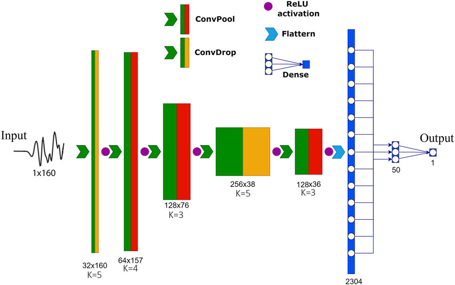
FIGURE 3. Architecture of the CFM, the deep Convolutional neural network for First Motion polarity classification used in this study. Numbers under each layer indicate its shape (i.e., number of channels x number of samples). ConvPool and ConvDrop indicate convolution with maxpooling and convolution with dropout, respectively. The values of K under each convolutional layer indicate the corresponding kernel size. The Flatten procedure (light blue arrow) only reshapes the previous layer in a one-dimensional array, without affecting any value.
We set the binary cross-entropy as the loss function to be minimized. To train the network, we used the Stochastic Gradient Descent (Robbins and Monro, 1951). SGD is one of the most simple and effective optimization methods widely used, and it can lead to better generalization performance compared to other more sophisticated methods. SGD is considered to play a central role in the observed generalization abilities of deep learning, since its stochasticity, resulting from the mini-batch sampling procedure, can provide a crucial implicit regularization effect (Ali et al., 2020). Moreover, the implicit regularization properties of SGD (Damian et al., 2021) are particularly useful when dealing with noisy data. We exploited the Stochastic Gradient Descend with the addition of Momentum. The default learning rate of
We set the maximum number of epochs to 100 and, to prevent overfitting, we implemented an early stopping technique that interrupts the training if there is no improvement in the validation loss for 7 consecutive epochs. Early stopping is also an effective implicit regularization technique, which has been observed to be surprisingly effective in preventing overfitting to mislabeled data, especially when used in combination with first-order optimization algorithms, such as SGD (Li et al., 2020).
4 Results
CFM was trained on waveforms outside blue and orange boxes in Figure 1A. The early stopping technique stopped the training at epoch number 20. We then evaluated the performance on the test set derived from dataset A (Figure 1A, blue box) and on the dataset B (Figure 1B), expressing it through confusion matrices (Figures 4A,B, respectively), showing the number of samples labeled consistently with the dataset (top-left and bottom-right) or oppositely (top-right and bottom-left). From them, we computed the accuracies, defined as the number of correct predictions divided by the total ones. The network reached accuracies of 97.4% and 96.3%, respectively.

FIGURE 4. Confusion matrices for dataset A (A) and dataset B (B) test sets. The x-axis shows network prediction, while the y-axis reports the labels present in the dataset. The accuracies for dataset A and dataset B are approximately 97.4% and 96.3%, respectively.
To provide a measure of the network’s reliability, we evaluated its behavior as the output varies on dataset A test set. A classifier is said to be ‘well-calibrated’ when its output probability can be directly interpreted as a confidence level (Dawid, 1982). For instance, a well-calibrated classifier should classify the samples such that among the samples to which it gave a predicted probability close to 0.8, approximately 80% actually belong to the positive class, which in our case is represented by upward polarity. Figure 5 represents a reliability diagram of our network (Niculescu-Mizil and Caruana, 2005), which indicates how often data points assigned a certain forecast output probability interval actually exhibit upward polarity (assigned in the dataset). Mathematically, the value of the height of the rectangle belonging to the bin
where
where
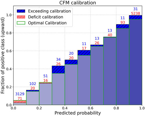
FIGURE 5. Reliability diagram of the network. Predictions made by the model are grouped into bins based on their predicted probabilities. The heights of the bars are the proportion of true positive cases within each bin. Green edges represent the average predicted probability of the bin, i.e., the optimal calibration. Numbers on each bar indicate the upward (red) and downward (blue) polarity waveforms laying in each bin.
4.1 CFM robustness to false annotations
We remember the SOM analysis of Section 3.1 revealed the presence of 337 waveforms with false labels (located within the nodes highlighted in Figure 2). Since the training set covers the majority of dataset A, the majority of these outlier waveforms (specifically 311) also belong to it. Despite the fact that the training algorithm forces the network output to match the assigned label, we found that 310 out of the 337 misclassified waveforms are assigned to the correct class by CFM. Figure 6 shows some examples of such waveforms we identified in Section 3.1 and for which the network predicts correct polarities. Given that the network successfully corrected 92% of the false labels, we consider this as evidence of its ability to be robust to overfitting erroneous labels.
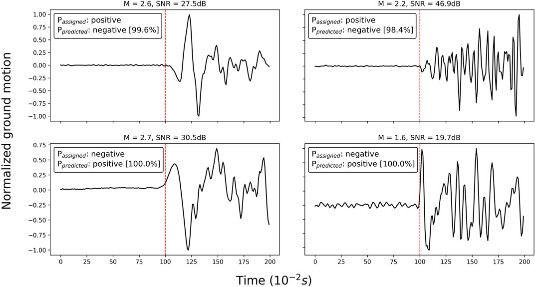
FIGURE 6. Some seismic traces erroneously labeled by the analyst that we identified with the SOM data visualization in Section 3.1. On the top of each subplot, we annotate the magnitude of the event (M) and the signal-to-noise ratio (SNR). Passigned and Ppredicted refer to the polarity assigned in the dataset and the prediction of the network (with the corresponding probability to belong to the predicted class in square brackets).
4.2 Dealing with uncertain arrival times
In this section, to check the robustness of the network to uncertainty in arrival times, we evaluated the performance of the network including artificial time shifts in arrival times. To this end, we shifted each time-window of dataset A test set by a constant value of T samples, with values of T in the range [-20,20]. A value of T = 5, for example, indicates that the time window center is located 5 samples (0.05 s) past the declared P-arrival. Red line in Figure 7 shows the behavior of the network (trained on centered time-windows) varying T as test sample-shift. We notice that, as expected, accuracy is highest when there is no shift. Accuracy rapidly declines, dropping to 50% when there is a shift of +10 samples, indicating a significant degradation in performance.
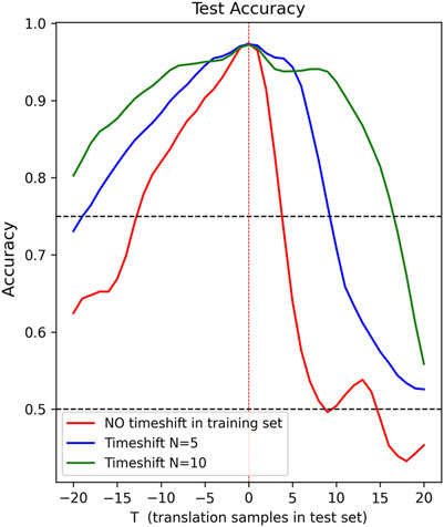
FIGURE 7. The performances of the CFM network on the test set after the two different training strategies. The blue and green lines refer to the trainings with a time-shift in the training set, with a maximum value N of 5 and 10 samples respectively. The red line shows the training without random time-shifts in the training set. Performance is shown as a function of the different shifts T in the test set. Dashed black lines refer to accuracy levels of 0.5 and 0.75.
Anyway, uncertainty in fixing the onset of P-wave is a trouble that often affects experimental data becoming much more difficult to manage for different reasons: poor signal-to-noise ratio, magnitude of the events decreases (small-energy/magnitude earthquake), recording stations installed in densely populated areas, complex medium properties, volcanic environment.
For this reason, we explored the possibility of giving the network the ability to deal with uncertainty in P-arrival times. Specifically, we developed an aimed augmentation strategy and performed a second training strategy, including a time-shift in the training set too. We used a time-shift augmentation procedure perturbing the centering of time windows contained in the training set, leaving the validation set unperturbed.
In particular, we selected 50% of the training waveforms and applied two independent uniform random time-shifts to each. The first time-shift was selected from the range [-N, −1], and the second from [1, N]. The original waveform and the two shifted versions were then included in the training set. We conducted two training sessions, on two augmented training sets, with N values of 5 and 10, respectively. Evaluating performance on unperturbed dataset A test set (T=0), we observe accuracy levels of 97.2% (in the case of N=10) and of 97.3% (in the case of N=5), which are slightly lower than the correspondent obtained by the model trained on unperturbed waveforms. However, as shown by the blue and green lines in Figure 7, adding time-shifts to the training set can lead to an improvement in performance in the presence of uncertain arrival times. In particular, we observed a broader plateau where the accuracy remains above 92.4%, even when dealing with shifts of 10 samples, in the case of N=10 (green line), and it takes 17 translation test samples to reduce the accuracy below 75%.
4.3 Model generalization ability
To evaluate the generalization ability of the CFM network, we checked the capability to generate accurate predictions on new datasets coming from completely different geographic regions (Southern California and western Japan regions), using recordings obtained by different seismic networks, and far from the region (Italy) on which the net was trained on.
We first utilized the SCSN test dataset provided by Ross et al. (2018). We excluded waveforms without assigned polarity, resulting in 863,151 traces suitable for our purposes. The network achieves an accuracy of 98.4% for waveforms with SNR greater than or equal to 10, while the accuracy is 96.3% for waveforms with a SNR less than 10. The overall accuracy is 97.5%, comparable to the model trained by Ross et al. (2018) on the SCSN dataset (i.e. 95%). Figure 8A shows the confusion matrix related to the network prevision on the SCSN dataset.
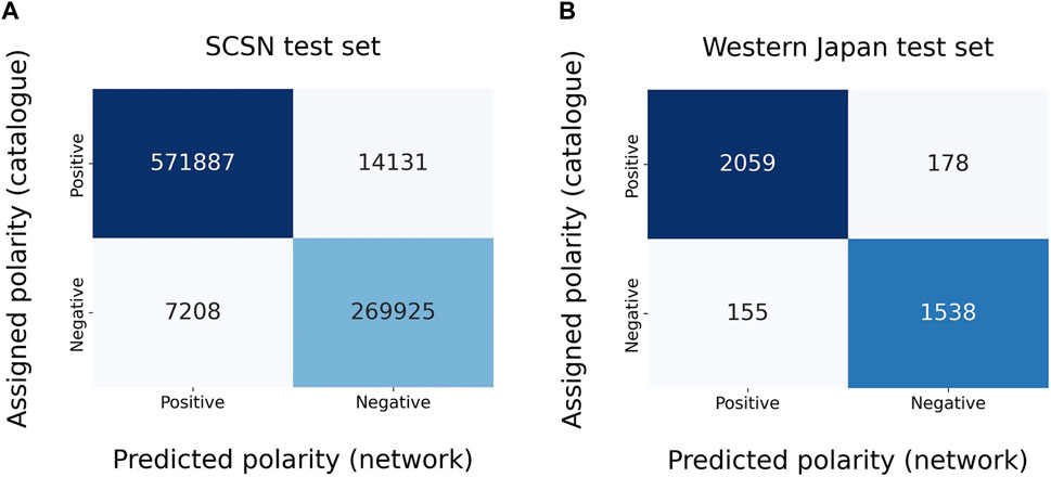
FIGURE 8. Confusion matrices for SCSN (A) and western Japan (B) test sets. The accuracies are approximately 97.5% and 91.5%, respectively. We recall that the performance on the western Japan test set refers to the different training using 150 as input waveforms.
We furthermore tested the performance on the test set provided by Hara et al. (2019), using only the 3,930 waveforms sampled at 100 Hz. We recall that CFM inputs are 160-sample waveforms, whereas the dataset we received contains 150-sample waveforms. Therefore, we have decided to conduct an additional training while keeping all the settings presented in the previous sections unchanged, except for the input shape, which we have adjusted to 150 samples to ensure compatibility. This additional training resulted in similar performances on both the dataset A and dataset B test sets when compared to the performance achieved with the 160-sample training. The predictions on the Hara et al. (2019) test set are presented in Figure 8B, from which one can compute an accuracy value of about 91.5%, slightly lower than the 95.4% obtained by the model of Hara et al. (2019).
5 Discussion
First-motion polarity determination can be a challenging task even for expert analysts, mainly when dealing with small-magnitude events, in both tectonic and volcanic environments. Deep learning neural networks have been widely applied in geophysics. Among many other applications, they have been used to detect first-motion polarities (Ross et al., 2018; Hara et al., 2019; Uchide, 2020; Chakraborty et al., 2022).
In this work, we developed the CFM network, a straightforward Convolutional Neural Network that can accurately identify the first-motion waveform polarity. Our results showed that CFM achieved a testing accuracy of 97.4% when applied to previously unseen traces. CFM also shows well generalization abilities, resulting in high accuracies on waveforms recorded from seismic networks located in completely different regions than those utilized to derive the training set (i.e., waveforms derived from the SCSN and western Japan test sets). For the SCSN test set, as noted in the previous works by Ross et al. (2018); Chakraborty et al. (2022), performance is better when dealing with waveforms that have a SNR greater than 10. Even if this is confirmed in our results, our network shows a gap in performance on different SNR of 2.1% when tested on SCSN test set, which is significantly lower than the 7.9% reported by Chakraborty et al. (2022). For the western Japan region, the accuracy achieved by CFM on the Hara et al. (2019) test set, at 91.5%, is slightly lower than the accuracies obtained on the other test sets and the one reported by Hara et al. (2019) themselves. However, a manual analysis of all 333 misclassified waveforms revealed that the polarity assigned in the test set was correct only in 29 cases, while for 59 waveforms the polarity identified by the model was correct. Other waveforms either presented ambiguous or unextractable polarity (119 waveforms) or had a considerable error in arrival time, up to 35 samples (126 waveforms). Supplementary Figure S5 provides a representation of the various cases. These findings confirm that the instances where the network does not perform well are remarkably limited, and its inferior performance cannot be attributed to shortcomings.
We observed that the employed implicit regularization strategies prevented the network from overfitting mislabeled data, resulting in the network’s ability to correct false labeling, even when the mislabeled waveforms are present in the training set. In line with previous studies (Uchide, 2020; Chakraborty et al., 2022), we demonstrated that implementing a time-shift augmentation procedure can lead to a decrease in performance when applied to unperturbed waveforms. However, unlike previous works, our additional training stages uncovered that an accurate augmentation procedure enables the handling of uncertainties in arrival times with only a minimal loss in performance on the unaltered data.
We also observe CFM exhibiting good calibration properties, which is critical for ensuring a high level of reliability in the model’s outputs, although we did not carry out any explicit calibration processes (Guo et al., 2017). In addition, we observe (Figure 5) that when the network works on waveforms with defined polarity, as in our case, the vast majority of outputs lie in the ranges [0, 0.1] for downward polarity and [0.9, 1] for upward polarity, resulting in high reliability. Due to its well-calibration properties, CFM is able to produce accurate probability estimates, enabling us to make informed decisions based on the output probability values. For example, a threshold can be introduced to determine when to accept or reject a prediction.
In conclusion, our study introduces the robust and highly adaptable CFM network that holds significant potential for determining the P-wave polarities. The generalization ability of the algorithm in producing accurate prediction on waveforms registered in regions different from those used to derive training data and its ability to rectify previously misclassified polarities are noteworthy contributions of this research. CFM key selling point lies in its capability to efficiently revise or validate large volumes of analyst-derived first-motion polarities in historic catalogs using a consistent method. It is important to note that the algorithm relies on phase arrival times and therefore cannot handle catalogs without this information. Although the application was presented on manually obtained picks, our findings suggest that the CFM network can easily be adapted downstream of the application of an automatic P-phase detection and labeling network, which is currently being worked on as a future development. This integration would enhance its adaptability and streamline the resolution of poorly-determined focal mechanisms in catalogs by quickly and robustly rectifying mislabeled first-motion polarities in databases. Overall, our research lays the foundation for further advancements in accurately characterizing tectonic and volcanic seismic events and improving our understanding of focal mechanisms.
Data availability statement
The datasets used in this study are publicly available for download. The INSTANCE dataset can be accessed at the following link: https://data.ingv.it/en/dataset/471#additional-metadata. The SCSN dataset is accessible at the following link: https://scedc.caltech.edu/data/deeplearning.html. The CFM network and dataset B used in this research can be found in the GitHub repository: https://github.com/Nemenick/CFM.git.
Author contributions
OA, SS, and PC conceived the work. GM performed all the analysis. GM and SS developed the algorithm and implemented the code. FN and OA prepared the seismic catalog. GM, FN, SS, OA, and MF worked on draft manuscript preparation. All authors contributed to the article and approved the submitted version.
Funding
PRIN-2017 MATISSE project, No. 20177EPPN2, funded by the Italian Ministry of Education and Research.
Acknowledgments
We thank Yukitoshi Fukahata for providing us with the dataset of Hara et al. (2019).
Conflict of interest
The authors declare that the research was conducted in the absence of any commercial or financial relationships that could be construed as a potential conflict of interest.
Publisher’s note
All claims expressed in this article are solely those of the authors and do not necessarily represent those of their affiliated organizations, or those of the publisher, the editors and the reviewers. Any product that may be evaluated in this article, or claim that may be made by its manufacturer, is not guaranteed or endorsed by the publisher.
Supplementary material
The Supplementary Material for this article can be found online at: https://www.frontiersin.org/articles/10.3389/feart.2023.1223686/full#supplementary-material
References
Ali, A., Dobriban, E., and Tibshirani, R. (2020). “The implicit regularization of stochastic gradient flow for least squares,” in International conference on machine learning (New York: PMLR), 233–244.
Alvizuri, C., and Tape, C. (2016). Full moment tensors for small events (M w< 3) at Uturuncu volcano, Bolivia. Geophys. J. Int. 206 (3), 1761–1783. doi:10.1093/gji/ggw247
Aoki, Y. (2022). Earthquake focal mechanisms as a stress meter of active volcanoes. Geophys. Res. Lett. 49 (19), e2022GL100482. doi:10.1029/2022GL100482
Bishop, C. M., and Nasrabadi, N. M. (2006). Pattern recognition and machine learning. New York: Springer.
Chakraborty, M., Cartaya, C. Q., Li, W., Faber, J., Rümpker, G., Stoecker, H., et al. (2022). PolarCAP–A deep learning approach for first motion polarity classification of earthquake waveforms. Artif. Intell. Geosciences 3, 46–52. doi:10.1016/j.aiig.2022.08.001
Chen, C., and Holland, A. A. (2016). PhasePApy: A robust pure Python package for automatic identification of seismic phases. Seismol. Res. Lett. 87 (6), 1384–1396. doi:10.1785/0220160019
Chiang, A., Dreger, D. S., Ford, S. R., and Walter, W. R. (2014). Source characterization of underground explosions from combined regional moment tensor and first-motion analysis. Bull. Seismol. Soc. Am. 104 (4), 1587–1600. doi:10.1785/0120130228
Dahm, T., and Brandsdóttir, B. (1997). Moment tensors of microearthquakes from the Eyjafjallajökull volcano in South Iceland. Geophys. J. Int. 130 (1), 183–192. doi:10.1111/j.1365-246X.1997.tb00997.x
Damian, A., Ma, T., and Lee, J. D. (2021). Label noise sgd provably prefers flat global minimizers. Adv. Neural Inf. Process. Syst. 34, 27449–27461. doi:10.48550/arXiv.2106.06530
Dawid, A. P. (1982). The well-calibrated Bayesian. J. Am. Stat. Assoc. 77 (379), 605–610. doi:10.1080/01621459.1982.10477856
Drory, A., Avidan, S., and Giryes, R. (2018). On the resistance of neural nets to label noise. arXiv preprint arXiv:1803.11410, 2.
Falanga, M., De Lauro, E., Petrosino, S., Rincon-Yanez, D., and Senatore, S. (2022). Semantically enhanced IoT-oriented seismic event detection: An application to Colima and Vesuvius volcanoes. IEEE Internet Things J. 9 (12), 9789–9803. doi:10.1109/JIOT.2022.3148786
Ford, S. R., Dreger, D. S., and Walter, W. R. (2009). Identifying isotropic events using a regional moment tensor inversion. J. Geophys. Res. Solid Earth 114 (B01306), 1–12. doi:10.1029/2008JB005743
Guo, C., Pleiss, G., Sun, Y., and Weinberger, K. Q. (2017). “July) on calibration of modern neural networks,” in International conference on machine learning (New York: PMLR), 1321–1330.
Hara, S., Fukahata, Y., and Iio, Y. (2019). P-wave first-motion polarity determination of waveform data in Western Japan using deep learning. Earth Planets Space 71 (1), 127. doi:10.1186/s40623-019-1111-x
Hardebeck, J. L., and Shearer, P. M. (2002). A new method for determining first-motion focal mechanisms. Bull. Seismol. Soc. Am. 92 (6), 2264–2276. doi:10.1785/0120010200
Judson, J., Thelen, W. A., Greenfield, T., and White, R. S. (2018). Focused seismicity triggered by flank instability on Kīlauea's Southwest Rift Zone. J. Volcanol. Geotherm. Res. 353, 95–101. doi:10.1016/j.jvolgeores.2018.01.016
Kiranyaz, S., Avci, O., Abdeljaber, O., Ince, T., Gabbouj, M., and Inman, D. J. (2021). 1D convolutional neural networks and applications: A survey. Mech. Syst. Signal Process. 151, 107398. doi:10.1016/j.ymssp.2020.107398
Kohonen, T. (2013). Essentials of the self-organizing map. Neural Netw. 37, 52–65. doi:10.1016/j.neunet.2012.09.018
Kong, Q., Wang, R., Walter, W. R., Pyle, M., Koper, K., and Schmandt, B. (2022). Combining deep learning with physics based features in explosion-earthquake discrimination. Geophys. Res. Lett. 49 (13), e2022GL098645. doi:10.1029/2022GL098645
Krizhevsky, A., Sutskever, I., and Hinton, G. E. (2017). Imagenet classification with deep convolutional neural networks. Commun. ACM 60 (6), 84–90. doi:10.1145/3065386
La Rocca, M., and Galluzzo, D. (2019). Focal mechanisms of recent seismicity at Campi Flegrei, Italy. J. Volcanol. Geotherm. Res. 388, 106687. doi:10.1016/j.jvolgeores.2019.106687
LeCun, Y., Bengio, Y., and Hinton, G. (2015). Deep learning. Nature 521 (7553), 436–444. doi:10.1038/nature14539
Li, M., Soltanolkotabi, M., and Oymak, S. (2020). “June). Gradient descent with early stopping is provably robust to label noise for overparameterized neural networks,” in International conference on artificial intelligence and statistics (New York: PMLR), 4313–4324.
Li, S., Fang, L., Xiao, Z., Zhou, Y., Liao, S., and Fan, L. (2023). FocMech-flow: Automatic determination of P-wave first-motion polarity and focal mechanism inversion and application to the 2021 yangbi earthquake sequence. Appl. Sci. 13 (4), 2233. doi:10.3390/app13042233
Linville, L., Pankow, K., and Draelos, T. (2019). Deep learning models augment analyst decisions for event discrimination. Geophys. Res. Lett. 46 (7), 3643–3651. doi:10.1029/2018GL081119
López-Pérez, M., García, L., Benítez, C., and Molina, R. (2020). A contribution to deep learning approaches for automatic classification of volcanovolcano-seismic events: Deep Gaussian processes. IEEE Trans. Geosci. Remote Sens. 59 (5), 3875–3890. doi:10.1109/TGRS.2020.3022995
Margheriti, L., Amato, A., Braun, T., Cecere, G., D'Ambrosio, C., De Gori, P., et al. (2013). Emergenza nell’area del Pollino: Le attività della Rete sismica mobile. Rapp. Tec. INGV 252, 1–40.
Michelini, A., Cianetti, S., Gaviano, S., Giunchi, C., Jozinović, D., and Lauciani, V. (2021). INSTANCE–the Italian seismic dataset for machine learning. Earth Syst. Sci. Data 13 (12), 5509–5544. doi:10.5194/essd-13-5509-2021
Miller, A. D., Julian, B. R., and Foulger, G. R. (1998). Three-dimensional seismic structure and moment tensors of non-double-couple earthquakes at the Hengill–Grensdalur volcanic complex, Iceland. Geophys. J. Int. 133 (2), 309–325. doi:10.1046/j.1365-246X.1998.00492.x
Mousavi, S. M., and Beroza, G. C. (2022). Deep-learning seismology. Science 377 (6607), eabm4470. doi:10.1126/science.abm4470
Napolitano, F., Amoroso, O., La Rocca, M., Gervasi, A., Gabrielli, S., and Capuano, P. (2021b). Crustal structure of the seismogenic volume of the 2010–2014 Pollino (Italy) seismic sequence from 3D P-and S-wave tomographic images. Front. Earth Sci. 9, 735340. doi:10.3389/feart.2021.735340
Napolitano, F., Galluzzo, D., Gervasi, A., Scarpa, R., and La Rocca, M. (2021a). Fault imaging at Mt Pollino (Italy) from relative location of microearthquakes. Geophys. J. Int. 224 (1), 637–648. doi:10.1093/gji/ggaa407
Niculescu-Mizil, A., and Caruana, R. (2005). “Predicting good probabilities with supervised learning,” in Proceedings of the 22nd international conference on Machine learning, New York, August 2005, 625–632. doi:10.1145/1102351.1102430
Passarelli, L., Roessler, D., Aladino, G., Maccaferri, F., Moretti, M., Lucente, F., et al. (2012). Pollino seismic experiment (2012-2014).
Perol, T., Gharbi, M., and Denolle, M. (2018). Convolutional neural network for earthquake detection and location. Sci. Adv. 4 (2), e1700578. doi:10.1126/sciadv.1700578
Pesicek, J. D., Sileny, J., Prejean, S. G., and Thurber, C. H. (2012). Determination and uncertainty of moment tensors for microearthquakes at Okmok Volcano, Alaska. Geophys. J. Int. 190 (3), 1689–1709. doi:10.1111/j.1365-246X.2012.05574.x
Prezioso, E., Sharma, N., Piccialli, F., and Convertito, V. (2022). A data-driven artificial neural network model for the prediction of ground motion from induced seismicity: The case of the Geysers geothermal field. Front. Earth Sci. 10, 2193. doi:10.3389/feart.2022.917608
Pugh, D. J., White, R. S., and Christie, P. A. F. (2016). Automatic Bayesian polarity determination. Geophys. J. Int. 206 (1), 275–291. doi:10.1093/gji/ggw146
Reasenberg, P. A. (1985). FPFIT, FPPLOT, and FPPAGE: Fortran computer programs for calculating and displaying earthquake fault-plane solutions. U. S. Geol. Surv. Open-File Rep., 85–739.
Richardson, A., and Feller, C. (2019). Seismic data denoising and deblending using deep learning. arXiv preprint arXiv:1907.01497. doi:10.48550/arXiv.1907.01497
Rincon-Yanez, D., De Lauro, E., Petrosino, S., Senatore, S., and Falanga, M. (2022). Identifying the fingerprint of a volcano in the background seismic noise from machine learning-based approach. Appl. Sci. 12 (14), 6835. doi:10.3390/app12146835
Robbins, H., and Monro, S. (1951). A stochastic approximation method. Ann. Math. Stat. 22, 400–407. doi:10.1214/aoms/1177729586
Rolnick, D., Veit, A., Belongie, S., and Shavit, N. (2017). Deep learning is robust to massive label noise. arXiv preprint arXiv:1705.10694. doi:10.48550/arXiv.1705.10694
Roman, D. C., Neuberg, J., and Luckett, R. R. (2006). Assessing the likelihood of volcanic eruption through analysis of volcanotectonic earthquake fault–plane solutions. Earth Planet. Sci. Lett. 248 (1-2), 244–252. doi:10.1016/j.epsl.2006.05.029
Ross, Z. E., Meier, M. A., and Hauksson, E. (2018). P wave arrival picking and first-motion polarity determination with deep learning. J. Geophys. Res. Solid Earth 123 (6), 5120–5129. doi:10.1029/2017JB015251
Rusiecki, A. (2020). “Standard dropout as remedy for training deep neural networks with label noise,” in Theory and applications of dependable computer systems: Proceedings of the fifteenth international conference on dependability of computer systems DepCoS-RELCOMEX, june 29–july 3, 2020, brunów, Poland (Germany: Springer International Publishing), 534–542. doi:10.1007/978-3-030-48256-5_52
Snoke, J. A., Lee, W. H. K., Kanamori, H., Jennings, P. C., and Kisslinger, C. (2003). Focmec: Focal mechanism determinations. Int. Handb. Earthq. Eng. Seismol. 85, 1629–1630. doi:10.1016/S0074-6142(03)80291-7
Song, H., Kim, M., Park, D., Shin, Y., and Lee, J. G. (2022). Learning from noisy labels with deep neural networks: A survey. IEEE Trans. Neural Netw. Learn. Syst., 1–19. doi:10.1109/TNNLS.2022.3152527
Uchide, T. (2020). Focal mechanisms of small earthquakes beneath the Japanese islands based on first-motion polarities picked using deep learning. Geophys. J. Int. 223, 1658–1671. doi:10.1093/gji/ggaa401
Uchide, T., Shiina, T., and Imanishi, K. (2022). Stress map of Japan: Detailed nationwide crustal stress field inferred from focal mechanism solutions of numerous microearthquakes. J. Geophys. Res. 127 (6), e2022JB024036. doi:10.1029/2022JB024036
Vavryčuk, V. (2014). Iterative joint inversion for stress and fault orientations from focal mechanisms. Geophys. J. Int. 199 (1), 69–77. doi:10.1093/gji/ggu224
Wang, S., Liu, W., Wu, J., Cao, L., Meng, Q., and Kennedy, P. J. (2016). “Training deep neural networks on imbalanced data sets,” in 2016 international joint conference on neural networks (IJCNN), Vancouver, 24-29 July 2016 (IEEE), 4368–4374. doi:10.1109/IJCNN.2016.7727770
Wéber, Z. (2018). Probabilistic joint inversion of waveforms and polarity data for double-couple focal mechanisms of local earthquakes. Geophys. J. Int. 213 (3), 1586–1598. doi:10.1093/gji/ggy096
Zhan, Y., Roman, D. C., Le Mével, H., and Power, J. A. (2022). Earthquakes indicated stress field change during the 2006 unrest of Augustine Volcano, Alaska. Geophys. Res. Lett. 49, e2022GL097958. doi:10.1029/2022gl097958
Zhao, L. S., and Helmberger, D. V. (1994). Source estimation from broadband regional seismograms. Bull. Seismol. Soc. Am. 84 (1), 91–104.
Zhao, M., Xiao, Z., Zhang, M., Yang, Y., Tang, L., and Chen, S. (2023). DiTingMotion: A deep-learning first-motion-polarity classifier and its application to focal mechanism inversion. Front. Earth Sci. 11, 335. doi:10.3389/feart.2023.1103914
Keywords: deep convolutional neural networks, automatic classification, machine learning, self-organizing maps, volcanic and tectonic earthquakes, first-motion polarity
Citation: Messuti G, Scarpetta S, Amoroso O, Napolitano F, Falanga M and Capuano P (2023) CFM: a convolutional neural network for first-motion polarity classification of seismic records in volcanic and tectonic areas. Front. Earth Sci. 11:1223686. doi: 10.3389/feart.2023.1223686
Received: 16 May 2023; Accepted: 10 July 2023;
Published: 20 July 2023.
Edited by:
Georg Rümpker, Goethe University Frankfurt, GermanyReviewed by:
Nishtha Srivastava, Frankfurt Institute for Advanced Studies, GermanyDarren Tan, University of Alaska Fairbanks, United States
Copyright © 2023 Messuti, Scarpetta, Amoroso, Napolitano, Falanga and Capuano. This is an open-access article distributed under the terms of the Creative Commons Attribution License (CC BY). The use, distribution or reproduction in other forums is permitted, provided the original author(s) and the copyright owner(s) are credited and that the original publication in this journal is cited, in accordance with accepted academic practice. No use, distribution or reproduction is permitted which does not comply with these terms.
*Correspondence: Giovanni Messuti, Zy5tZXNzdXRpQHN0dWRlbnRpLnVuaXNhLml0; Ortensia Amoroso, b2Ftb3Jvc29AdW5pc2EuaXQ=