- 1Exploration and Development Research Institute of Petro China Southwest Oil and Gas Field Company, Chengdu, China
- 2College of Resources and Security, Chongqing University, Chongqing, China
Since the discovery of the Carboniferous gas reservoirs in East Sichuan in 1977, after more than 40 years of development, most of the gas reservoirs have entered the middle and late stages of development. The gas reservoir is characterized by strong heterogeneity, large difference in permeability, and serious impact of water invasion in some blocks. Therefore, how to make a correct decision on gas field development and deployment is of vital importance. Combined with system clustering, BP neural network, correlation analysis and other methods, this paper first analyzes and calculates the static indicators of the Carboniferous gas reservoirs, and then divides the gas reservoirs into four categories using ward clustering method according to the calculated weight value, and determines the characteristics of each type of gas reservoirs using correlation coefficient analysis method. Finally, the recovery prediction model of each type of gas reservoir is established according to the BP neural network. The results indicate that: (1) The recovery rate prediction model can predict the trend of cumulative gas production changes, thereby obtaining the space for improving recovery rate, and the accuracy of the prediction results is high, which can be used as a reference for gas field planning. (2) The sub-active gas reservoirs with strong heterogeneous water bodies and the inactive gas reservoirs with low permeability water bodies have a certain space for enhanced oil recovery.
1 Introduction
With the development of society and economy, China’s demand for natural gas is increasing. At the same time, the pressure of energy consumption control and environmental protection is also increasing. In order to alleviate these problems, an efficient and reasonable gas field development policy is crucial (Zhang. et al., 2022). The results of national oil and gas resources evaluation during the 13th Five-Year Plan show that the natural gas resources in Sichuan Basin are the first in China, and the discovery rate of natural gas resources is only 15%, which is still in the early and middle stages of exploration. Therefore, Sichuan Basin has great potential for natural gas development and is the primary target of natural gas exploration planning at present (Zhang, 2022). The Carboniferous strata are widely distributed in the east of Sichuan, and many high-yield gas fields have been found so far, which become the main production reservoir in the east of Sichuan. However, the carboniferous gas reservoir in the east of Sichuan is also one of the most complicated gas reservoirs in China. It is characterized by complex structure, deep burial, multiple formation pressure systems, strong heterogeneity, large permeability difference, and severe water invasion in some blocks (Ailin et al., 2017; Hu. et al., 2020). After more than 40 years of development since 1977, most of the Carboniferous gas reservoirs in eastern Sichuan have entered the middle and late stage of exploitation, so how to make the right decision on gas field development and deployment has a crucial role.
In order to better complete the analysis of gas reservoir development indicators, and play a guiding role in gas field development and deployment decision-making, big data analysis and neural network prediction methods should be fully applied. Due to the different controlling factors of recovery efficiency in different types of carboniferous gas reservoirs, it is necessary to quantitatively characterize the influencing factors, classify the gas reservoirs according to the influencing factors, and determine the main characteristics of each type of gas reservoir. In addition, the Sichuan Basin has a large number of gas reservoirs with various types and a long history of development. The existing recovery efficiency evaluation methods are mostly based on experience, analogy and formula, which can not well meet the needs of gas field development planning. Therefore, it is necessary to carry out the research of gas reservoir recovery efficiency prediction model based on big data, so as to realize the recovery efficiency prediction of gas reservoirs in different life cycles (Liu. et al., 2021; Luo. et al., 2022; Makhotin. et al., 2022).
At present, there are qualitative and quantitative analysis methods for the quantitative representation of influencing factors. In order to display the strength of influencing factors more accurately, quantitative mathematical representation methods, such as risk regression method and weight calculation method, are needed. P. Antao (Antão et al., 2023) combined the Bayesian algorithm and the least square method to evaluate the impact of six risk factors such as length and type on collision probability according to the historical data of collision accidents worldwide. The results show that the risk factors that have a greater impact on ship collision are type and geographical region. Changping Li (Li. et al., 2021) used the Extreme learning machine (a single hidden layer feedforward neural network algorithm) to analyze the weight of six influential factors such as peak voltage and electrode spacing on the probability of electrical breakdown. The correlation and contribution of each influencing factor to the electric breakdown probability are obtained, which provides guidance and basis for the design of electrode drill bit and the selection of drilling process parameters in different strata. With reference to these research methods, it is advisable to use neural network for weight calculation. The multi-layer perceptron neural network has high precision and is more sensitive to weight calculation (Gurgel et al., 2022; Luo. et al., 2023), so it is suitable for quantitative characterization of the influencing factors of recovery efficiency.
At present, there are many methods about clustering analysis, such as systematic clustering method, hierarchical clustering method, fuzzy clustering method and so on (Li. et al., 2022; Wang et al., 2022). Among them, the system clustering method further calculates the relationship between various factors, can be more efficient and accurate classification of objective elements, therefore, the system clustering method is suitable for gas reservoir classification, its core algorithm is Ward method. Adam Lurka (Adam, 2021) used Ward minimum variance method to make a systematic cluster analysis of mining induced earthquakes. Cluster analysis of mining seismic activity provides a new method for determining focal groups and high stress zones in the rock mass in the mine, so as to determine earthquake and rockburst hazards. Yu Ogasawara (Yu and Masamichi, 2021) proposed two clustering methods based on Ward method, using interval value dissimilarity for interval value data. The results show that the proposed clustering method can intuitively provide reasonable and consistent results for the sample data, and the results of the clustering method using interval value dissimilarity can be fully understood through the arrow tree diagram. Brooke E. Husic (Husic and Pande, 2017) proposed a clustering method using Ward minimum variance objective function to predict new data points, and combined Ward method with six other clustering algorithms to generate cross-validation scores for MSM constructed from protein-folding datasets. The Ward method minimizes the sum of square distances and shows that there is a correspondence between the objective function based on variance or mean value and the optimal division of protein conformational space.
At present, it is common to use neural network for prediction research. The main methods of neural network model prediction include feedforward neural network, feedback neural network and AD hoc network (Shoaib. et al., 2018; Lan and Zhang., 2019; Qu. et al., 2020). Cristiano Hora Fontes (Hora Fontes and Embiruçu, 2021) proposed a new weight initialization method combined with construction algorithm to construct a feedforward neural network for multi-class classification. Compared with the traditional random weight initialization method, this method can be widely used in the synthesis of multi-class classification problem reference and real data sets. Marta Kolasa (Marta et al., 2018) implemented an effective initialization method for neuron weights in AD organized networks on hardware, and found that self-organized maps can be trained without initialization, which reduces the complexity of applying AD organized neural networks. Haitao Li (Li, 2019) applied BP neural network optimized based on firefly swarm algorithm to predict network traffic, and achieved good prediction effect with high prediction accuracy, and opened up a good application prospect in this field. Dachao Yuan (Yuan. et al., 2014) used BP neural network model and RBF neural network model built by Matlab to predict coal mine gas emission data, and the results showed that BP neural network had higher prediction accuracy. For the settlement problem of highway soft foundation, Yi Xue (Yi et al., 2011) applied BP neural network and three-point method to predict soft foundation settlement. The results show that BP neural network can effectively avoid the human error in the three-point method, and has higher prediction accuracy, with smaller settlement error. BP neural network has the advantages of strong adaptability, high precision and strong fault tolerance, which is suitable for the research of gas reservoir recovery efficiency prediction.
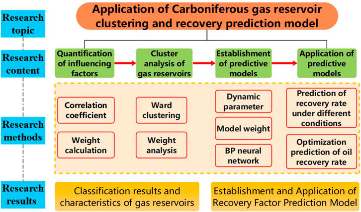
In this paper, geological factors are screened for carboniferous gas reservoirs in eastern Sichuan, and static indexes affecting recovery are determined. Then, the weight of static indexes of each gas reservoir is calculated by multi-layer sensor, and the preliminary analysis of gas reservoirs is carried out. Then combined with the weight value of static index, Ward clustering method was used for cluster analysis of carboniferous gas reservoirs, and the correlation coefficient was calculated to obtain the characteristics of each type of gas reservoirs, which served as the basis for subsequent modeling. Finally, the recovery efficiency training model of each kind of gas reservoir is established based on BP neural network, and the boundary conditions are set. The recovery efficiency prediction model is established by combining the actual data and the weight obtained by training, so as to predict the change trend of future recovery efficiency and the change of recovery efficiency after changing the dynamic parameters. At the same time, the sensitivity analysis of dynamic parameters can be carried out. Determine the optimal results of dynamic parameters of each type of gas reservoir. Figure 1 is a flow chart of the research work.
2 Quantitative characterization of influencing factors
2.1 Determination of influencing factors and quantitative methods
2.2.1 Determination of influencing factors of recovery efficiency
Geological factors and development policy factors affect gas reservoir recovery. Among them, geological factors include reservoir physical property, heterogeneity, gas-water relationship, water energy and so on. Development policy factors include production rate, well pattern density, well type, and potential exploitation measures.
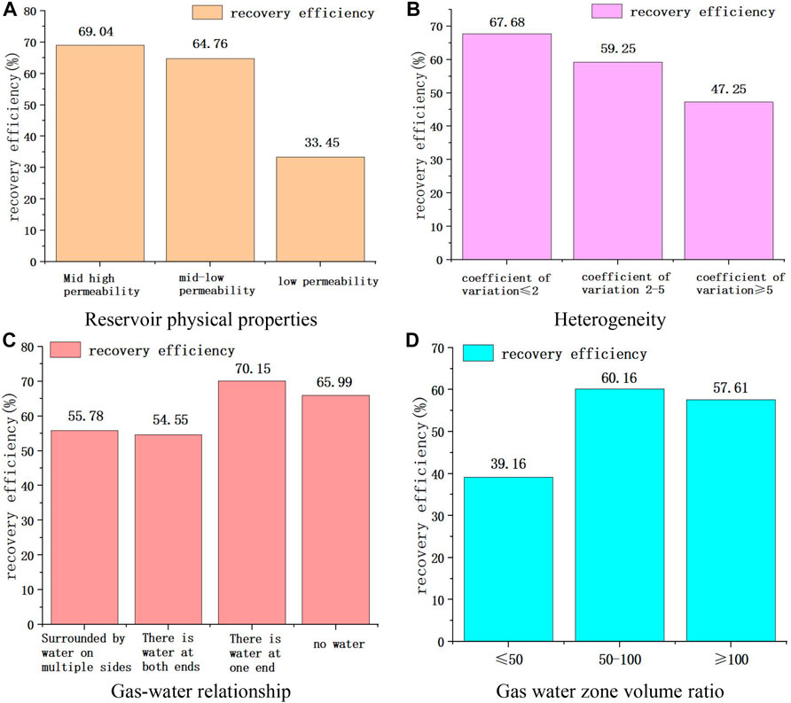
Figure 2 shows the comparative results of recovery efficiency under different geological conditions. It can be seen from the figure that the recovery efficiency of gas reservoirs with different reservoir physical properties is significantly different, and the recovery efficiency of medium-high permeability gas reservoirs is much higher than that of low-permeability gas reservoirs. The heterogeneity of gas reservoir is characterized by coefficient of variation, and the recovery efficiency of gas reservoir with small coefficient of variation is higher. For the gas-water relationship, the average recovery of gas reservoirs surrounded by water and with water at both ends of the structure is lower than that of gas reservoirs with water at one end of the structure or without water. Gas reservoirs with high water energy (gas-water volume ratio of 50 or less) generally have lower average recovery than other gas reservoirs.
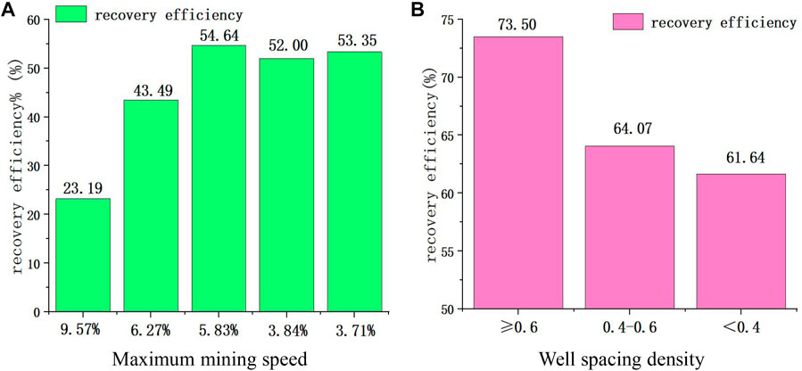
Figure 3 shows the comparison results of recovery efficiency under different development conditions. It can be seen from the figure that the higher the production rate, the lower the recovery efficiency of gas reservoirs, and the average recovery efficiency of gas reservoirs with production rate greater than 6% is generally lower than 50%. The recovery efficiency of gas reservoirs with different well pattern densities varies greatly. The average recovery efficiency of gas reservoirs with well pattern densities greater than or equal to 0.6 Wells/km2 exceeds 70%. In addition, by comparing the recovery efficiency under different technological measures and potential measures, it can be seen that the higher the proportion of process well, the greater the recovery efficiency of gas reservoir; Developing gas production technology and pressurized gas transmission technology can improve gas reservoir recovery.
Among these influencing factors, the index of correlation is selected as the characterization of the influencing factors of recovery efficiency. Among them, geological factors do not change with time, which is a static index, while development policy factors change with time, which is a dynamic index. After screening, there are 10 static indexes, which are permeability, porosity, effective fracture density, formation coefficient, energy storage coefficient, coefficient of variation, transverse distance between gas reservoir and gas-water interface (referred to as transverse distance), longitudinal distance between gas reservoir and gas-water interface (referred to as longitudinal distance), gas-water area ratio (referred to as area ratio) and gas-water volume ratio (referred to as volume ratio). There are five dynamic indicators, which are production rate, well pattern density, water gas ratio, wellhead oil pressure and process well ratio.
2.2.2 Research on quantitative characterization methods of influencing factors
The quantitative characterization methods of influencing factors include Pearson correlation coefficient method and neural network weight calculation method.
Correlation coefficient method mainly studies the degree of correlation between two variables, and the calculation formula is shown in Eq. 1 (Sun. et al., 2023).
In the formula, r is the correlation coefficient, n is the number of data points, and
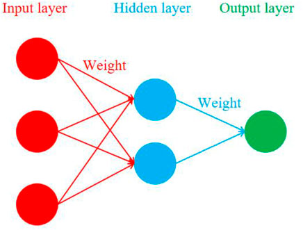
The core idea of neural network weight method is: when multiple factors have coupling influence on a variable, multi-layer perceptron is used to calculate the weight value of each factor. The greater the weight value, the greater the influence of the factor. The structure of the multi-layer perceptron is shown in Figure 4. It includes input layer, hidden layer and output layer, and the layers are connected by weights. The hidden layer contains two activation functions: sigmoid function and tanh function. The calculation formula is shown in Eqs. 2, 3.
2.2 Weight analysis of influencing factors of gas reservoir
Before classifying Carboniferous gas reservoirs, the weights of static indicators of each gas reservoir should be calculated, and the gas reservoirs should be classified according to geological factors. Therefore, 10 static indicators are used as the input layer and the output layer is the recovery factor of the gas reservoir, which is replaced by the cumulative gas production.
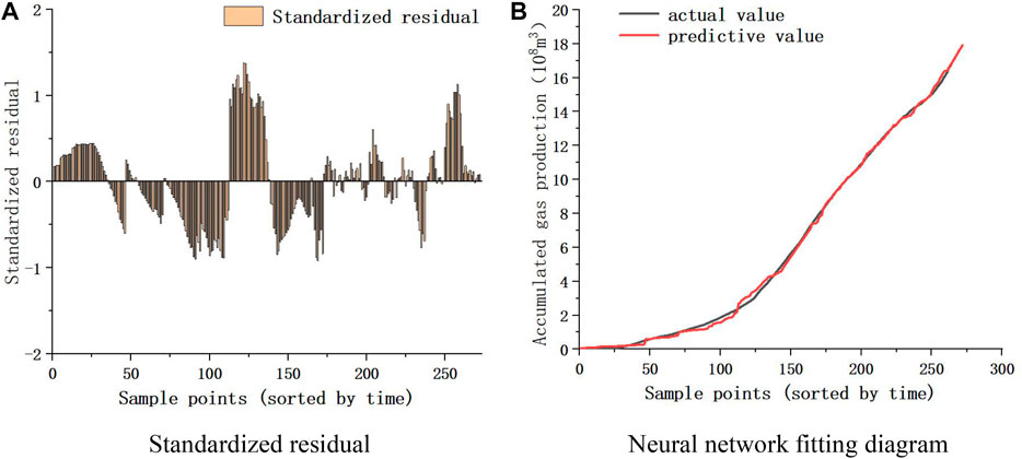
SPSS software was used for neural network calculation to obtain the weight value of the influencing factors and the residual value of the calculation results. Specific ideas are as follows: Firstly, all static parameters and historical data of cumulative gas production are input, and then each parameter is set in the variable view. Then, the multi-layer perceptron of the neural network is selected for weight calculation, in which the cumulative gas production is the output end and the other 10 static indicators are the input end. Finally, the automatic adjustment hidden layer is selected in the architecture, and the standardized residual error of the sample points is compared after calculation. According to the t-test in the residual test, when the standardized residual is [-2, 2], the error is small and there is no outlier (Mohammed and Muhammad, 2021; Muhammad et al., 2021). As can be seen from Figure 5A and Figure 4B, the error of calculation results is small, and the predicted value and actual value of neural network have a high degree of fitting.
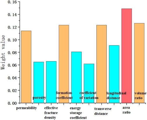
Figure 5 is the neural network calculation result diagram of FJW gas reservoir. After calculation, the residual diagram (left figure) and the result fitting diagram (right figure) are analyzed, and it can be seen that the residual value is small and the degree of fitting is high, indicating that the results under the calculation condition are relatively accurate. Therefore, the calculation result is selected as the static index weight of FJW, and the weight value of each index is shown in Figure 6.
The larger the weight value, the higher the degree of influence of the factors. Based on the height of the weight value, the main influencing factors of the gas reservoir are determined, thereby obtaining the main characteristics of the gas reservoir and establishing a foundation for subsequent gas reservoir classification. As shown in Figure 6, the main influencing factors of FJW are permeability, formation coefficient, and gas-water relationship, indicating that the water body of FJW is active. In addition, different colors in the figure represent the strength of the factors, with red indicating the factor with the greatest impact, yellow indicating the factor with the greater impact, and blue indicating the factor with the lesser impact.
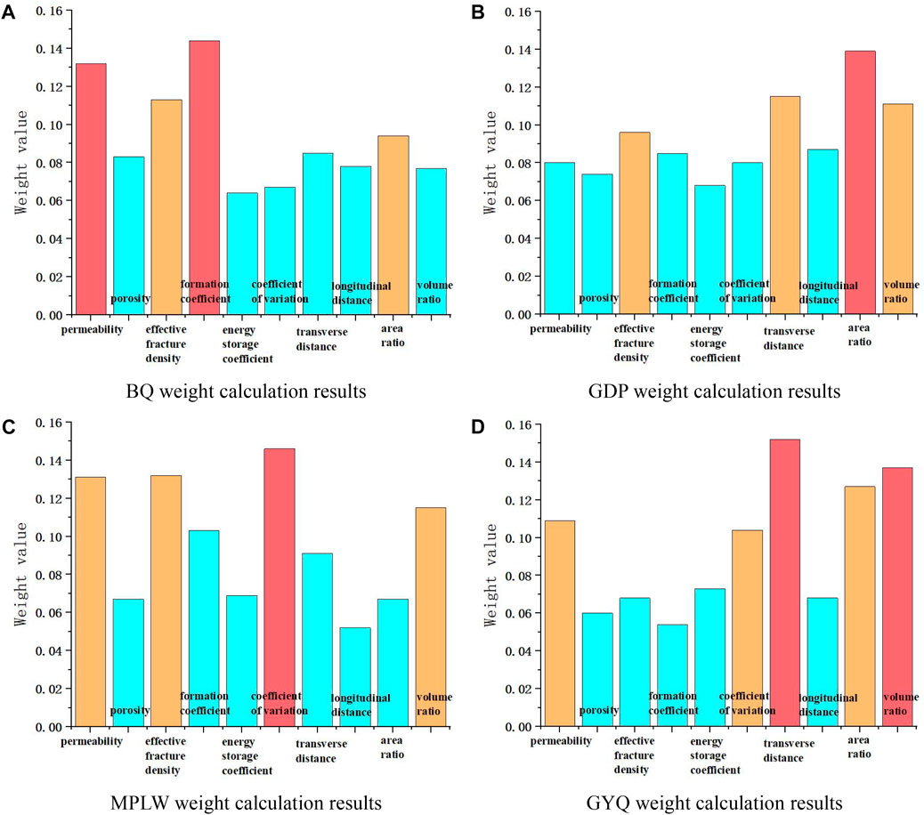
According to the above calculation process, static index weights were calculated for 40 Carboniferous gas reservoirs, among which several representative calculation results were selected, as shown in Figure 7.
Figure 7 shows the weight calculation results for some gas reservoirs. The weight values have been normalized, and the sum of all weights equals one. On the one hand, a larger weight value indicates a greater degree of impact, and on the other hand, the main impact indicators are determined based on the relative size of the weight. Select the three to five factors with the highest weight for each gas reservoir as the main influencing factors for the gas reservoir. Below, based on the calculation results, the main factors of the four gas reservoirs will be explained separately.
For BQ Carboniferous system, the indicators that have the greatest influence include formation coefficient, permeability and effective fracture density, indicating that the main influencing factor of this gas reservoir is reservoir physical property, which belongs to low seepage body inactive gas reservoir.
For GDP Carboniferous system, the most influential indicators include: gas-water area ratio, lateral distance, gas-water volume ratio, indicating that the gas reservoir is mainly affected by the occurrence state of gas and water, which belongs to the medium-high water seepage volume ∼ inactive gas reservoir.
For MPLW Carboniferous system, the most influential indicators include: coefficient of variation, effective fracture density, permeability, gas-water volume ratio, indicating that the main influencing factors of this gas reservoir are reservoir physical property and heterogeneity, belonging to the sub-active gas reservoir with heterogeneous water.
For GYQ Carboniferous system, the most influential indicators include: lateral distance, gas-water volume ratio, gas-water area ratio, indicating that the main influencing factors of this gas reservoir are water energy and gas-water occurrence state, which belongs to active water gas reservoir.
According to the strength of influencing factors of different gas reservoirs, the policy of enhancing oil recovery can be put forward reasonably. For example, in medium-strong water flooding and medium-high permeability gas reservoirs, the main strategy to improve oil recovery is to control drainage and production as a whole, and the most relevant indicators are the corresponding average wellhead oil pressure, drainage well/production well, measure well ratio, etc. The main strategy to improve oil recovery in medium-strong water drive and heterogeneous gas reservoirs is to evaluate multi-round infilling and drainage gas production. The most relevant indicators are the corresponding total number of Wells, well pattern density, proportion of horizontal Wells, number of producing Wells and other related indicators. The main measures to improve oil recovery in weak water drive and medium-high permeability gas reservoirs are rational production allocation and pressurized production, and the highest correlation indexes are annual gas production, production rate and average wellhead oil pressure. The main strategy to improve oil recovery in weak water drive and heterogeneous low permeability gas reservoirs is to evaluate multiple rounds of infilling, and the most relevant indexes are the corresponding well pattern density, effective fracture density, porosity and other related indexes.
This is because the main EOR strategies are different for different gas reservoirs. The main countermeasures of medium-strong water drive and medium-high permeability gas reservoirs are drainage and production control as a whole. The main countermeasures of medium-strong water drive and heterogeneous gas reservoirs are gas recovery through evaluation of multi-round filling and drainage. The main countermeasures of weak water drive and medium-high permeability gas reservoirs are rational production allocation and pressurized production. The main countermeasure of weak water drive and heterogeneous low permeability gas reservoir is to evaluate multiple rounds of infilling.
Different recovery enhancement strategies lead to different levels of sensitivity of the cumulative gas production of gas reservoirs to each index, which is reflected in the algorithm, that is, the speed of updating and iteration of the weight value is different, and finally leads to the difference in the weight of each index of different types of gas reservoirs. Because each gas reservoir has different characteristics and each index has different influence on the recovery factor, it is necessary to classify the gas reservoir according to the weight of static index, and then determine the characteristics of each kind of gas reservoir, and then carry out the prediction research of gas reservoir recovery factor.
3 Cluster analysis of gas reservoirs
3.1 Ward clustering method and correlation analysis
Ward method is the sum of squares of deviation method. The idea is that the sum of squares of class deviations is smaller and the sum of squares of deviations between classes is larger. The Ward method always combines classes in such a way that the increment of the sum of the squares within the class caused by the union class is minimized. The Ward method finally grouped the variables with smaller distances into one class, and the calculated distance adopted was Euclidean distance. The calculation formula was shown in Eq. (4).
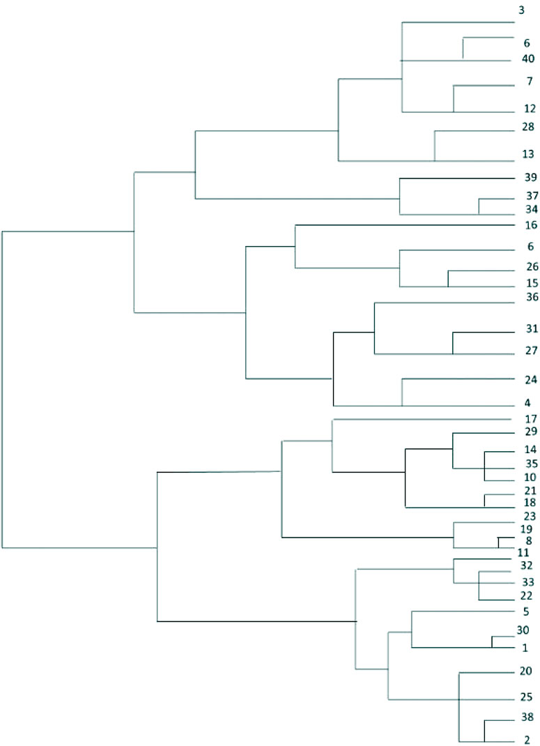
After the weight calculation of static indicators is completed, 40 gas reservoirs of the Carboniferous system are numbered according to the weight values obtained. Then, ward clustering method is used to classify gas reservoirs. Finally, clustering diagram is obtained according to the classification results, as shown in Figure 8.
Figure 8 shows the classification results of gas reservoirs. The ward clustering method is used to calculate the distance of gas reservoir features based on weight values. The closer the distance is, the closer the position in the graph is. The gas reservoirs are numbered from 1 to 40, and the specific classification situation is determined based on the numbering. From right to left, based on the numbers on the right, 2 and 38 can be considered the same type. They have some differences from 20 to 25, but compared to 1 and 30, 2, 38, 20, and 25 can be considered the same type. Finally, based on the classification diagram, gas reservoirs are divided into four categories according to static indicators. The characteristics of each type of gas reservoir are determined by the correlation coefficient method, and the correlation analysis results are shown below.
The correlation coefficients of the first gas reservoir are shown below.
Table 1 shows the correlation coefficients (r) of the first type of gas reservoir. According to 2.2.2, when r>0.7, it is a strong correlation, when 0.4<r<0.7, it is a moderate correlation, and when 0.2<r<0.4, it is a weak correlation. When determining the characteristics of gas reservoirs, only strong and medium correlations are considered. Based on the calculated correlation coefficients, the relevant indicators of each type of gas reservoir are determined to determine the characteristics of the gas reservoir.
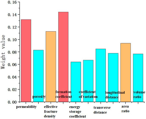
According to the data in Table 1, in the first type of gas reservoir, the strong correlation indexes of the cumulative gas production are permeability, porosity, effective fracture density and formation coefficient. The medium correlation indexes are: area ratio of gas-water zone, volume ratio of gas-water zone, longitudinal distance and transverse distance. It can be inferred that the main influencing factors of this kind of gas reservoir are reservoir physical properties, and the secondary influencing factors are the occurrence state of gas and water and water energy.
Figure 9 shows the static index weight of the first class gas reservoir. It can also be seen from the figure that the largest proportion of weight is permeability, effective fracture density and formation coefficient, which also correspond to the main influencing factors of gas reservoir - reservoir physical property.
The correlation coefficients of the second gas reservoir are shown below.
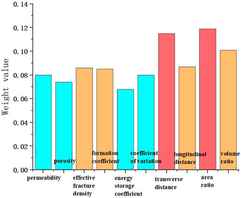
From the data in Table 2, it can be seen that in the second type of gas reservoir, the strong correlation indexes of cumulative gas production are: gas-water area ratio; Medium correlation indexes are: gas - water volume ratio, lateral distance. It can be inferred that the main influencing factor of this kind of gas reservoir is the occurrence state of gas and water, and the secondary influencing factor is water energy.
Figure 10 shows the static index weight of the second type of gas reservoir. It can also be seen from the figure that the largest proportion of weight is the horizontal distance, the area ratio of gas-water zone and the volume ratio of gas-water zone, which also correspond to the occurrence state of gas and water, the main influencing factor of gas reservoir.
The correlation coefficients of the third type of gas reservoir are shown below.
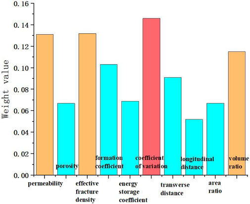
According to the data in Table 3, in the third type of gas reservoir, the strong correlation indexes of the cumulative gas production include formation coefficient, permeability, effective fracture density, and coefficient of variation. The medium correlation index is: gas-water zone volume ratio. It can be inferred that the main influencing factors of this kind of gas reservoir are reservoir physical property and heterogeneity, and the secondary influencing factors are water energy.
Figure 11 shows the static index weights of the third type gas reservoir. It can also be seen from the figure that the largest proportion of weights are permeability, coefficient of variation and effective fracture density, which also correspond to the main influencing factors of gas reservoir - reservoir physical property and coefficient of variation.
The correlation coefficient table of the fourth type gas reservoir is shown below.
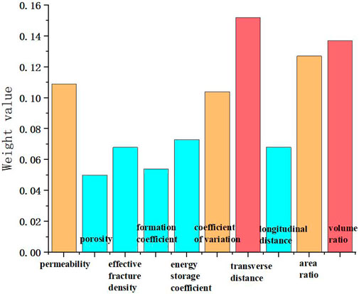
According to the data in Table 4, in the fourth type of gas reservoir, the strong correlation indexes of cumulative gas production are: gas-water area ratio and gas-water volume ratio; Intermediate correlation indexes are: lateral distance, permeability, coefficient of variation. It can be inferred that the main influencing factor of this kind of gas reservoir is the occurrence state of water body energy and gas water, and the secondary influencing factor is reservoir physical property.
Figure 12 shows the static index weight of the fourth type gas reservoir. It can also be seen from the figure that the largest proportion of weight is horizontal distance, area ratio of gas-water zone and volume ratio of gas-water zone, which also correspond to the main influencing factors of gas reservoir water energy and gas-water occurrence state.
3.2 Analysis of gas reservoir clustering results
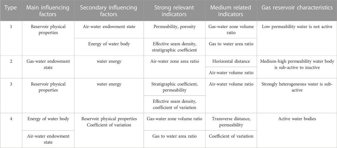
The classification of gas reservoirs based on the degree of influence factors is formed by quantifying the static index weights of gas reservoirs, combined with ward clustering method. Pearson’s coefficient was used to discern the major influences (r > 0.7) and minor influences (r between 0.4 and 0.7) for different types of gas reservoirs. Table 5 shows the statistical table of gas reservoir classification and evaluation based on the degree of influence of factors.
According to the correlation coefficient calculation results in 3.1, the main and secondary influencing factors of each type of gas reservoir are obtained, as shown in Table 5. Among them, the gas-water relationship mainly represents the activity of the water body. The larger the volume and area ratio of the gas-water zone, the more active the water body is. The formation coefficient, permeability, and other factors are mainly proportional to the heterogeneity of the gas reservoir. Finally, the characteristics of each type of gas reservoir are determined based on the nature of the water body and the heterogeneity of the gas reservoir. The results of gas reservoir classification are as follows.
The first category of gas reservoirs belongs to low permeability water body inactive gas reservoirs, including: BQ, FXC, ZJC, SCP, LYP, PX, BJC, WSK, GX, LB, XHK, TS, TMC, SGP, WLH, FJW, WQJ, TZP.
The static index range is as follows. Reservoir physical properties: permeability 0.1∼1 mD, porosity 3–5%, effective fracture density 2–5/m, formation coefficient 1–30, energy storage coefficient 0.5–1; heterogeneity: coefficient of variation 1–5; gas-water relationship: vertical distance 20–100 m, horizontal distance 100–200 m, gas-water area ratio 0.3–1; water energy: gas water area volume ratio of 100–200. Main influencing factors: reservoir physical properties. Main influencing factors: reservoir physical properties. Secondary influencing factors: gas water occurrence state, water energy.
The second type of gas reservoir belongs to the sub-inactive gas reservoir with medium and high permeability, including GDP, WSC, SMZ, XGS, FCZ and ZGW.
The static index range is as follows. Reservoir physical properties: permeability 5–30 mD, porosity 5–7%, effective fracture density 10–15/m, formation coefficient 100–500, energy storage coefficient 0.5–2; heterogeneity: coefficient of variation 1–2; gas-water relationship: longitudinal distance 50–250 m, transverse distance 200–600 m, gas-water area ratio 1–4; water energy: gas-water volume ratio 200–1,000. Main influencing factors: gas water occurrence state. Secondary influencing factors: water energy.
The third type of gas reservoir belongs to the heterogeneous water sub-active gas reservoir, including LT, MPLW, MYB, XJG, HJB, DPY, TSB, SPC and WBT.
The static index range is as follows. Reservoir physical properties: permeability 1–10 mD, porosity 5–8%, effective fracture density 5–10/m, formation coefficient 30–150, energy storage coefficient 0.5–2; heterogeneity: coefficient of variation 1–10; gas-water relationship: longitudinal distance 10–50 m, transverse distance 100–200 m, gas-water area ratio 0.05–0.3; water energy: gas water area volume ratio 5–100. The main influencing factors: reservoir physical properties, heterogeneity. Secondary influencing factors: water energy.
The fourth type of gas reservoir belongs to the water active gas reservoir, including: GYQ, GFC, SJB, YHZ, WLS, CYS.
The static index range is as follows. Reservoir physical properties: permeability 5–30 mD, porosity 5–6%, effective fracture density 10–15/m, formation coefficient 50–300, energy storage coefficient 2–5; heterogeneity: coefficient of variation 1–10; gas-water relationship: longitudinal distance 5–10 m, transverse distance 100–200 m, gas-water area ratio 0.1–0.5; water energy: gas water area volume ratio of 30–100. Main influencing factors: water energy, gas and water occurrence state. Secondary influencing factors: reservoir physical properties, coefficient of variation.
After completing the clustering of gas reservoirs and obtaining the characteristics of each type of gas reservoirs, combined with the static index weight value, the recovery prediction model of each type of gas reservoirs is established, and the training and prediction are completed to test the prediction results. After determining the accuracy of the model, the model is used to predict the cumulative gas production trend of each gas reservoir and explore the maximum value of gas reservoir recovery. At the same time, the sensitivity analysis of dynamic indexes of different types of gas reservoirs can be carried out to clarify the variation law of gas reservoir recovery under different mining conditions, which can be used to guide the development of gas reservoirs.
4 Establishment and application of recovery prediction model
4.1 Theoretical basis of recovery prediction model
The prediction model of gas reservoir recovery includes two parts: training model and prediction model.
1) Establishment of training model:
Step 1:. Import input x (dynamic and static parameters), give output t (cumulative gas production), and start training. The transfer function from the input layer to the hidden layer is:
Where x is the input information, y is the calculation result of the hidden layer, and wij is the weight value from the input layer to the hidden layer.Remarks: ① The weights of 10 static parameters are calculated according to the previous calculation, and remain unchanged. The weights of dynamic parameters are calculated according to the hidden layer. ② When the dynamic parameters are input, the time series is added to make the cumulative gas production increase with time.The transfer function from the hidden layer to the output layer is:
Where z is the output result and wjk is the weight value from the hidden layer to the output layer.
Step 2:. Calculate the error and adjust the weight value.t is the initial given output, that is, the actual value of cumulative gas production, and z is the model output result. The error between the network output and the target output is:
When the error is greater than the set value (5% of the cumulative gas production), the weight value is adjusted to reduce
Step 3:. Complete the iterative calculation and establish the training model.Adjust the weight to make the error less than the set value, complete the training and output the results. The process of weight adjustment is called iteration. The complete iterative process is as follows: The iterative formula of weight adjustment is:
Here, uj is the input of the jth neuron in the hidden layer:
The jth neuron of the hidden layer is connected to each neuron of the output layer, that is, ∂ε/∂ yj involves all weights wij, so
Finally, the weight is adjusted according to the simplified Eq. 13 until the end of training, and the gas reservoir recovery training model is obtained.
1) Establishment of prediction model:
According to the established training model, the recovery rate prediction is studied.In order to accurately predict recovery (cumulative gas production), constraints need to be considered:Data boundary conditions: the upper limit of cumulative gas production, abandoned production (1000 m3) and the lower limit of minimum pressure (0.2 MPa) are controlled by dynamic reserves.2) Mapping conditions: Input the final time node of the prediction, take the month as the step size, automatically calculate the result of each step from the end of the fitting section to the input time node, and form the prediction curve.
The prediction module follows the following steps. Input data normalization: Because the range of some input data of the neural network may be particularly large, the neural network converges slowly and the training time is long. Therefore, the data need to be preprocessed before training the neural network. An important preprocessing method is normalization. It is to map the data to [0, 1] or [−1, 1] interval or smaller interval. A simple and fast normalization algorithm is linear transformation algorithm. The formula is as follows:In the formula: y is the normalized output vector; x is the input vector; min is the minimum value of x; max is the maximum value of x.Loading neural network: Let the input mode of the network is
Where yj is the output of the jth neuron in the hidden layer,
The transfer function above is the activation function, which is de-linearized. The calculation of the neural network nodes is the weighted sum, plus the bias term:
This is a linear model, the calculation results will be passed to the next node or the same linear model. Only through linear transformation, all the hidden layer nodes have no meaning of existence. The reason is as follows: Suppose that the weight matrix of each layer is represented by
In the formula: y is the output vector after denormalization; x is the input vector; min is the maximum value of x; max is the maximum value of x.
4.2 Establishment of recovery prediction model
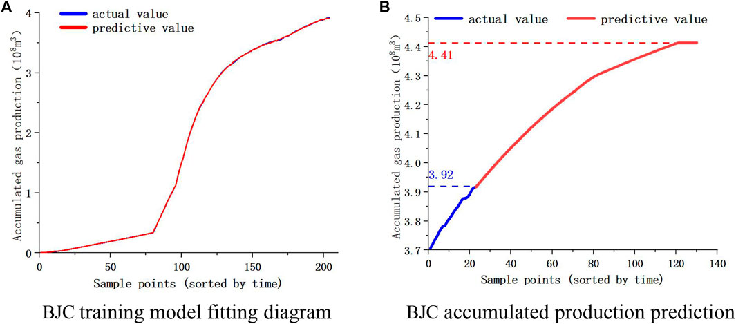
The principle of the recovery rate prediction model is described in 4.1, and the establishment process of the prediction model is detailed below. Firstly, all historical data of the gas reservoir, including geological factors, development factors, and cumulative gas production, are substituted, and the cumulative gas production is set as output and trained using a BP neural network. After repeated weight iteration calculations, a training model with the required error will be established, and the first step of modeling is completed. Then, based on the actual situation, set the boundary conditions of the model, such as the limit range of wellhead oil pressure and production rate, the time for gas reservoir development, etc., and combine the training model and formula (18) to establish a recovery rate prediction model. Below is a detailed explanation using BJC gas reservoir as an example in the first type of gas reservoir.
In the first step, the weight value of the static index is used as a fixed value to participate in the calculation, and the historical data is trained. After the calculation, the weight value of the dynamic index will be returned. Because the neural network calculation process is built-in calculation of the computer, only the calculation results can be derived, so the calculation of the software is taken as an example to illustrate. The number of training times is the number of weight adjustment times when the set training module performs error analysis. A total of 200 different training models are obtained by adjusting the weight 200 times, and then the training model with the smallest difference from the actual value of the historical data is selected as the final output. Among them, the activation function selects tanh because it is relatively stable. Similarly, it is also possible to select the sigmoid function and get different training models.
Figure 13A is the fitting diagram of the output results and historical data of the training model. The higher the fitting degree, the closer the training model is to the real value, the higher the accuracy, and the greater the reliability of the prediction. In the process of calculation, the weight value of static parameters is obtained by the previous calculation, fixed and directly involved in the calculation; the weight values of the dynamic parameters are calculated by the hidden layer and are constantly changing with the calculation. These weight values are also directly involved in the calculation of the neural network. After the training model is established, the weight values are all determined. When the new data is input for prediction, the weight values of the training model are calculated.
Then the prediction model. When predicting, it is necessary to input the actual value of dynamic parameters and the final time node of prediction. For example, the dynamic parameters remain unchanged and are predicted to December 2040, as shown in Figure 13B.
In the calculation, the cumulative gas production prediction value of each node is calculated with the monthly step, and the curve is connected to view the change trend of cumulative gas production. In addition, the calculation is in accordance with the order of time series, from front to back in order to predict, so that the cumulative gas production to maintain a monotonically increasing trend. The specific calculation formula is as described in the prediction section of 4.1. At each time node, these formulas are calculated in the hidden layer according to these formulas, and the weight value is determined in the training model. Finally, the prediction results are all output and form a graph, which is the cumulative gas production prediction result.
4.3 Verification and application of recovery prediction model
The recovery factor prediction model established is mainly applied by software, and the accuracy of the model is verified with examples. The verification results of some Carboniferous gas reservoirs are as follows. It can be seen from Table 6. 1) On the whole, the error between the training results and the prediction results of the model is low, and the error is only 5.3%, indicating that the model has high accuracy and strong adaptability. 2) The smaller the error of the training model, the smaller the error of the prediction results. Before using the model to predict, we must try to ensure that the training model has a high degree of fitting and ensure the accuracy of the prediction.
Finally, the gas reservoir recovery prediction software is compiled by matlab. The software is composed of three cores: training module, prediction module and sensitivity analysis. It can realize three functions: history matching of different types of gas reservoirs, recovery prediction under different mining conditions and sensitivity analysis.
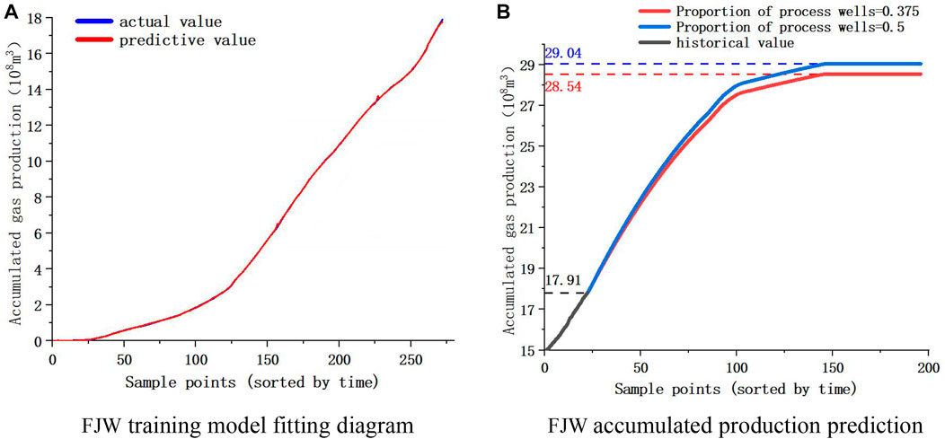
Taking FJW gas reservoir as an example, the historical data is first trained and the model is established. Figure 14A is the training result of historical data. From the diagram, it can be seen that the training data and the actual data fit well, indicating that the training effect is good and the accuracy of the model is relatively high.
Figure 14B is the prediction curve of cumulative gas production. The black curve in the figure is the historical yield; the red curve is the prediction curve of cumulative gas production when the current mining conditions remain unchanged (the proportion of process wells is 0.375). The blue curve is the prediction curve of cumulative gas production when the mining conditions are changed (other conditions remain unchanged, the proportion of process wells increases to 0.5).
As shown in the figure, the cumulative gas production will maintain the existing growth rate for growth, and the growth curve will gradually become gentle at a certain time in the future, and reach the maximum cumulative gas production. If the current mining conditions are maintained, the cumulative gas production will increase from 17.91×10⁸ m3 to 28.54×10⁸ m3, and then reach the maximum value and stop production. If the mining conditions are changed, the proportion of process wells will increase from 0.375 to 0.5, and the final cumulative gas production will increase from 28.54×10⁸ m3 to 29.04×10⁸ m3, thereby increasing recovery.
Finally, the software can also be used to calculate the recovery rate of different types of gas reservoirs under the change of dynamic index.
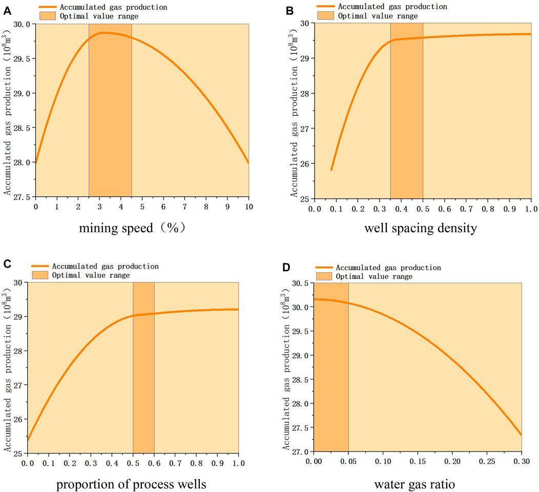
1) The first type of gas reservoir (low permeability water body inactive gas reservoir) under different development conditions, the change of cumulative gas production is shown in Figure 15. The sensitivity analysis of different dynamic indicators is as follows. Mining speed: The cumulative gas production increases first and then decreases with the increase of mining speed, and the optimal range is 2.5–4.5%. Well spacing density: The cumulative gas production increases first and then slows down with the increase of well spacing density, and finally tends to be stable. The optimal range is 0.35–0.5wells/km2. The proportion of process wells: the cumulative gas production increases first and then slows down with the increase of the proportion of process wells, and finally tends to be stable. The optimal range is 0.5–0.6. The water-gas ratio: the smaller the water-gas ratio, the greater the cumulative gas production, and the cumulative gas production decreases slowly first and then decreases rapidly with the increase of water-gas ratio. The optimal range is 0–0.05m3/104 m3.
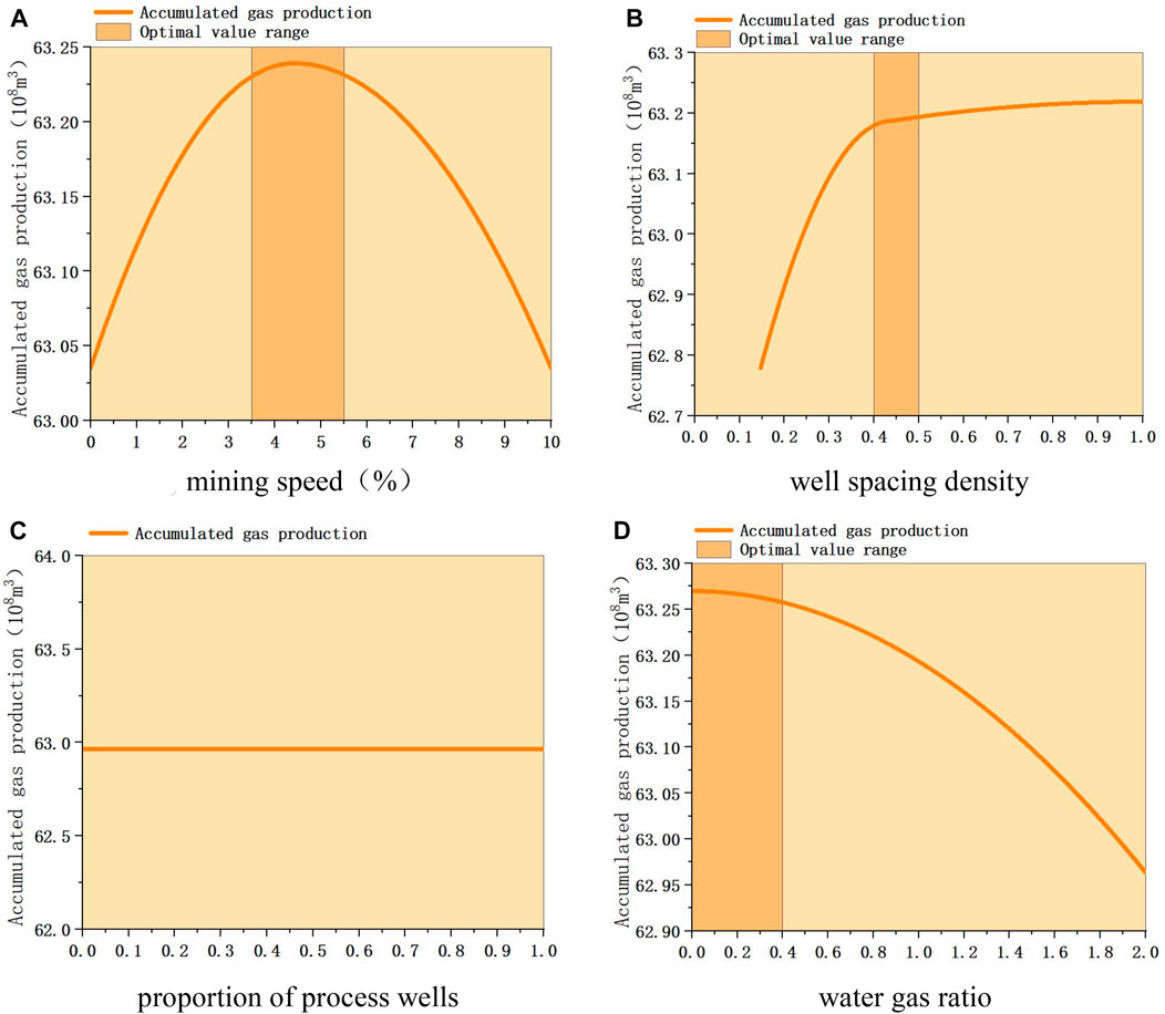
2) The second type of gas reservoir (medium-high permeability water body inactive gas reservoir) under different development conditions, the change of cumulative gas production is shown in Figure 16. The sensitivity analysis of different dynamic indicators is as follows. Mining speed: The cumulative gas production increases first and then decreases with the increase of mining speed, and the optimal range is 3.5–5.5%. Well spacing density: The cumulative gas production increases first and then slows down with the increase of well spacing density, and finally tends to be stable. The optimal range is 0.4–0.5wells/km2. The proportion of process wells: the cumulative gas production of gas reservoirs has nothing to do with the implementation of process wells. The water-gas ratio: the smaller the water-gas ratio, the greater the cumulative gas production, and the cumulative gas production decreases slowly first and then decreases rapidly with the increase of water-gas ratio. The optimal range is 0–0.4m3/104 m3.
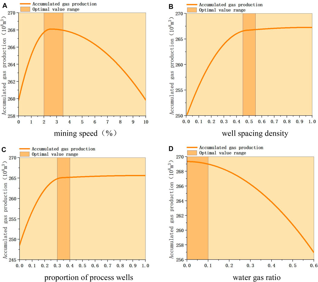
3) The change of cumulative gas production of the third type of gas reservoir (strong heterogeneity water sub-active gas reservoir) under different development conditions is shown in Figure 17. The sensitivity analysis of different dynamic indicators is as follows. Mining speed: The cumulative gas production increases first and then decreases with the increase of mining speed, and the optimal range is 2–3.5%. Well spacing density: The cumulative gas production increases first and then slows down with the increase of well spacing density, and finally tends to be stable. The optimal range is 0.45–0.55wells/km2. The proportion of process wells: the cumulative gas production increases first and then slows down with the increase of the proportion of process wells, and finally tends to be stable. The optimal range is 0.3–0.4. The water-gas ratio: the smaller the water-gas ratio, the greater the cumulative gas production, and the cumulative gas production decreases slowly first and then decreases rapidly with the increase of water-gas ratio. The optimal range is 0–0.1m3/104 m3.
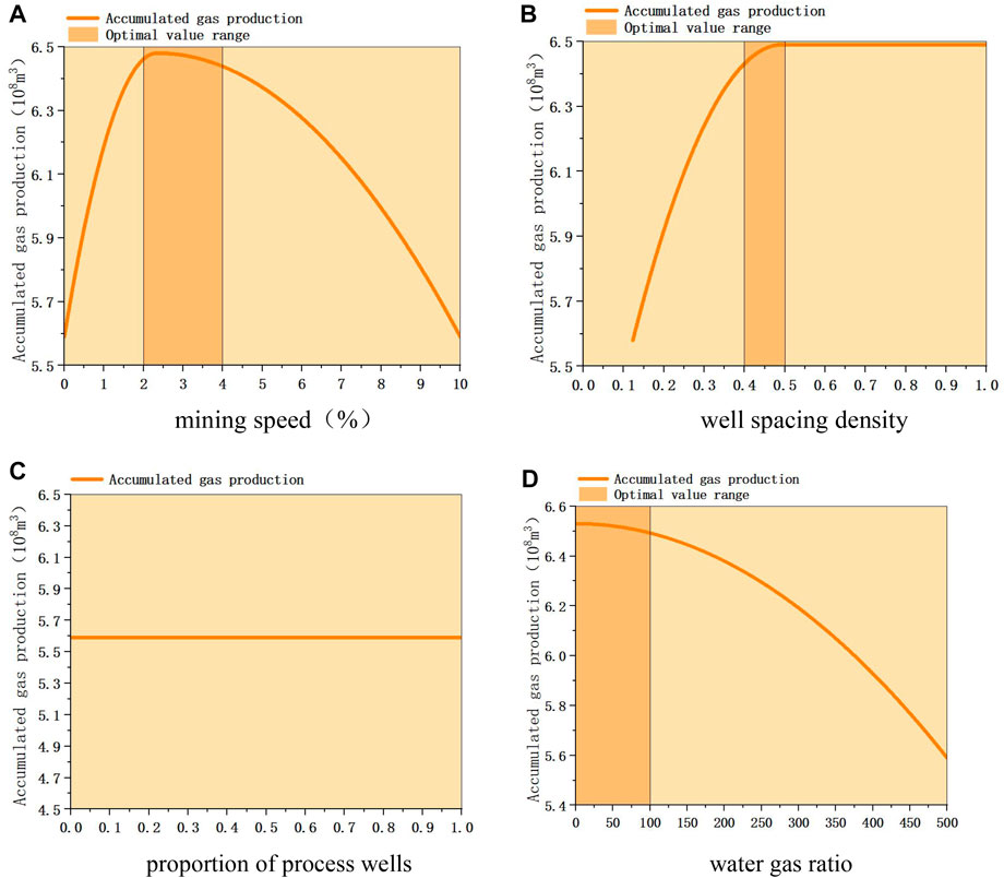
4) The fourth type of gas reservoir (water active gas reservoir) under different development conditions, the change of cumulative gas production is shown in Figure 18. The sensitivity analysis of different dynamic indicators is as follows. Mining speed: The cumulative gas production increases first and then decreases with the increase of mining speed, and the optimal range is 2–4%. Well spacing density: The cumulative gas production increases first and then slows down with the increase of well spacing density, and finally tends to be stable. The optimal range is 0.4–0.5wells/km2. The proportion of process wells: the cumulative gas production of gas reservoirs is not related to the implementation of process wells. The water-gas ratio: the smaller the water-gas ratio, the greater the cumulative gas production, and the cumulative gas production decreases slowly at first and then decreases rapidly with the increase of water-gas ratio. The optimal range is 0–100m3/104 m3. The water-gas ratio of this kind of gas reservoir is large, indicating that the influence of water invasion is serious, so the overall water control of gas reservoir is necessary.
Finally, according to the model and the change law of cumulative gas production, the optimal solution of dynamic index is input into four types of gas reservoirs for calculation, and the recovery rate of four types of gas reservoirs can be improved, as shown in Table 7. Then, we combine the remaining geological reserves to evaluate, evaluation criteria: the remaining geological reserves >200×108 m3, the average recovery space >3% of the gas reservoir type evaluation for space. The evaluation results show that the sub-active gas reservoirs with strong heterogeneous water bodies and the inactive gas reservoirs with low permeability water bodies also have a certain space for enhanced oil recovery. This conclusion provides a reference for the next work deployment of enhanced oil recovery and the optimization of gas reservoirs with potential.
5 Conclusion
1) The geological environment of Carboniferous gas Sichuan is complex, and there are many factors affecting oil recovery. Different types of Carboniferous gas reservoirs have different main controlling factors. In view of this feature, this paper uses multi-layer perceptron to calculate the weight value of the static index of the gas reservoir. Based on this, the ward method is used to cluster the gas reservoir, and the characteristics of each type of gas reservoir are obtained. Then the recovery factor prediction model is established. After example verification, the accuracy of the model is guaranteed. Finally, using the established recovery model, the maximum recovery rate of each gas reservoir under different conditions can be predicted. At the same time, the sensitivity analysis of the dynamic index is carried out, and the space for improving the recovery rate of different types of gas reservoirs under the optimal conditions is clarified. The results show that the sub-active gas reservoir with strong heterogeneous water body and the inactive gas reservoir with low permeability water body also have a certain space for enhanced oil recovery. This conclusion plays an important role in making correct gas field development and deployment decisions.
2) Starting from the main controlling factors of recovery factor, this paper studies the influence degree of geological factors on recovery factor of each gas reservoir, completes the cluster analysis of gas reservoir, and finally establishes models for gas reservoirs with different characteristics. This research model provides a new idea for the study of gas reservoir recovery. Especially for gas reservoirs with complex geological structure, strong heterogeneity and large permeability difference, the influencing factors of recovery are complex. In the case of multi-factor coupling, it is difficult to determine the classification and main controlling factors of gas reservoirs. Therefore, the combination of neural network and system clustering can effectively solve these problems. At the same time, the established recovery prediction model is suitable for the Carboniferous gas reservoirs in eastern Sichuan, which can realize the recovery prediction and recovery optimization prediction under different mining conditions, and has a guiding role in the subsequent development of gas reservoirs.
Data availability statement
The original contributions presented in the study are included in the article/supplementary material, further inquiries can be directed to the corresponding author.
Author contributions
ZK has collected and organized literature, providing technical support; PX provided data and processed it; YiC and YY have identified and improved research methods; QM proposed a holistic research approach and identified research steps; DZ has completed the establishment and validation of the model and applied it to practical engineering; YC summarized all research and analyzed the results obtained, and wrote an article. All authors contributed to the article and approved the submitted version.
Conflict of interest
KZ, XP, YC, YY, QM was employed by the Petro China Southwest Oil and Gas Field Company.
The remaining authors declare that the research was conducted in the absence of any commercial or financial relationships that could be construed as a potential conflict of interest.
Publisher’s note
All claims expressed in this article are solely those of the authors and do not necessarily represent those of their affiliated organizations, or those of the publisher, the editors and the reviewers. Any product that may be evaluated in this article, or claim that may be made by its manufacturer, is not guaranteed or endorsed by the publisher.
References
Adam, L. (2021). Spatio-temporal hierarchical cluster analysis of mining-induced seismicity in coal mines using Ward's minimum variance method. J. Appl. Geophys. 184, 104249. doi:10.1016/j.jappgeo.2020.104249
Ailin, J., Dewei, M., and Dongbo, H. (2017). Technical measures of deliverability enhancement for mature gas fields: A case study of carboniferous reservoirs in wubaiti gas field, eastern Sichuan Basin, SW China. Petroleum Explor. Dev. 44, 615–624.
Antão, P., Sun., S., Teixeira, A. P., and Guedes Soares, C. (2023). Quantitative assessment of ship collision risk influencing factors from worldwide accident and fleet data. Reliab. Eng. Syst. Saf. 234, 109166. doi:10.1016/j.ress.2023.109166
Gurgel, V., Mahmoud, D., Meneghetti Ugulino de Araújo., F., and da Silva Guerra, M. I. (2022). Comparing multilayer perceptron and probabilistic neural network for PV systems fault detection. Expert Syst. Appl. 201, 117248. doi:10.1016/j.eswa.2022.117248
Hora Fontes, C., and Embiruçu, M. (2021). An approach combining a new weight initialization method and constructive algorithm to configure a single Feedforward Neural Network for multi-class classification. Eng. Appl. Artif. Intell. 106, 104495. doi:10.1016/j.engappai.2021.104495
Husic, B. E., and Pande, V. S. (2017). Ward clustering improves cross-validated markov state models of protein folding. J. Chem. Theory Comput. 13, 963–967. doi:10.1021/acs.jctc.6b01238
Hu., Y., Xian, P., Qian, L., Li, L., and Hu, D. (2020). Progress and development direction of technologies for deep marine carbonate gas reservoirs in the Sichuan Basin. Nat. Gas. Ind. B 7, 149–159. doi:10.1016/j.ngib.2019.09.004
Lan, X., and Zhang., Y. (2019). Quality prediction model based on novel elman neural network ensemble. Complexity 2019, 1–11. doi:10.1155/2019/9852134
Li, H. (2019). Network traffic prediction of the optimized BP neural network based on Glowworm Swarm Algorithm. Syst. Sci. Control Eng. 72, 64–70. doi:10.1080/21642583.2019.1626299
Li., C., Duan., L., Kang., J., Li, A., Xiao, Y., and Chikhotkin, V. (2021). Weight analysis and experimental study on influencing factors of high-voltage electro-pulse boring. J. Petroleum Sci. Eng. 205, 108807. doi:10.1016/j.petrol.2021.108807
Liu., Y., Xin-Hua, M., Zhang, X., Guo, W., Kang, L. X., Yu, R. Z., et al. (2021). A deep-learning-based prediction method of the estimated ultimate recovery (EUR) of shale gas wells. Petroleum Sci. 18, 1450–1464. doi:10.1016/j.petsci.2021.08.007
Li., Y., Yang., G., Luo., W., Zhou, Y., Hu, R., Liu, Y., et al. (2022). Research on EV loads clustering analysis method for source-grid-load system. Energy Rep. 8, 718–722. doi:10.1016/j.egyr.2022.10.354
Luo., M., Bhandari., B., Li., H., Aberdeen, S., and Lee, S. S. (2023). Efficient lens design enabled by a multilayer perceptron-based machine learning scheme. Optik 273, 170494. doi:10.1016/j.ijleo.2022.170494
Luo., S., Xu., T., and Shuijian, W. (2022). Prediction method and application of shale reservoirs core gas content based on machine learning. J. Appl. Geophys. 204, 104741. doi:10.1016/j.jappgeo.2022.104741
Makhotin., I., Denis, O., Koroteev., D., Burnaev, E., Karapetyan, A., and Antonenko, D. (2022). Machine learning for recovery factor estimation of an oil reservoir: A tool for derisking at a hydrocarbon asset evaluation. Petroleum 8, 278–290. doi:10.1016/j.petlm.2021.11.005
Marta, K., Rafał, D., Tomasz, T., and Pedrycz, W. (2018). Efficient methods of initializing neuron weights in self-organizing networks implemented in hardware. Appl. Math. Comput. 319, 31–47. doi:10.1016/j.amc.2017.01.043
Mohammed, A., and Muhammad, A. (2021). Testing internal quality control of clinical laboratory data using paired t-test under uncertainty. BioMed Res. Int. 2021, 5527845. doi:10.1155/2021/5527845
Muhammad, A., Bantan., R. A. R., and Khan., N. (2021). Design of tests for mean and variance under complexity-an application to rock measurement data. Measurement 177, 109312. doi:10.1016/j.measurement.2021.109312
Qu., N., Chen., J., Zuo., J., and Liu, J. (2020). PSO–SOM neural network algorithm for series arc fault detection. Adv. Math. Phys. 2020, 1–8. doi:10.1155/2020/6721909
Shoaib., M., Shamseldin., A. Y., Khan., S., Khan, M. M., Khan, Z. M., Sultan, T., et al. (2018). A comparative study of various hybrid wavelet feedforward neural network models for runoff forecasting. Water Resour. Manage 32, 83–103. doi:10.1007/s11269-017-1796-1
Sun., J., Song, R., Shang., Y., Zhang, X., Liu, Y., and Wang, D. (2023). A novel fault prediction method based on convolutional neural network and long short-term memory with correlation coefficient for lithium-ion battery. J. Energy Storage 62, 106811. doi:10.1016/j.est.2023.106811
Wang, H. Y., Wang, J. S., and Guan, W. (2022). A survey of fuzzy clustering validity evaluation methods. Inf. Sci. 618, 270–297. doi:10.1016/j.ins.2022.11.010
Yi, X., Cao., Z., and Shan, L. (2011). The application of BP neural network in settlement prediction of highway soft foundation. Adv. Mater. Res. 250, 3440–3443. doi:10.4028/www.scientific.net/amr.250-253.3440
Yu, O., and Masamichi, K. (2021). Two clustering methods based on the Ward's method and dendrograms with interval-valued dissimilarities for interval-valued data. Int. J. Approx. Reason. 129, 103–121. doi:10.1016/j.ijar.2020.11.001
Yuan., D., Yue., X., Chen, W., and Zhang, J. F. (2014). Gas emission prediction based on coal mine operating data. Appl. Mech. Mater. 484, 604–607. doi:10.4028/www.scientific.net/amm.484-485.604
Zhang, D. (2022). Development prospect of natural gas industry in the Sichuan Basin in the next decade. Nat. Gas. Ind. B 9, 119–131. doi:10.1016/j.ngib.2021.08.025
Keywords: carboniferous gas reservoir, systematic clustering, correlation analysis, BP neural network, recovery factor prediction
Citation: Zhang K, Peng X, Chen Y, Yan Y, Mei Q, Chen Y and Zhang D (2023) Cluster analysis of carboniferous gas reservoirs and application of recovery prediction model. Front. Earth Sci. 11:1220189. doi: 10.3389/feart.2023.1220189
Received: 10 May 2023; Accepted: 01 June 2023;
Published: 12 June 2023.
Edited by:
Yubing Liu, China University of Mining and Technology, ChinaReviewed by:
Weijing Xiao, East China Jiaotong University, ChinaXian-meng Zhang, Shijiazhuang Tiedao University, China
Copyright © 2023 Zhang, Peng, Chen, Yan, Mei, Chen and Zhang. This is an open-access article distributed under the terms of the Creative Commons Attribution License (CC BY). The use, distribution or reproduction in other forums is permitted, provided the original author(s) and the copyright owner(s) are credited and that the original publication in this journal is cited, in accordance with accepted academic practice. No use, distribution or reproduction is permitted which does not comply with these terms.
*Correspondence: Yu Chen, MjAyMjIwMDEwMDdAc3R1LmNxdS5lZHUuY24=
 Kai Zhang1
 Yu Chen
 Dongming Zhang