Constraints on the structure of the oceanic crust of the Tamu Massif by teleseismic P-wave coda autocorrelation

The Tamu Massif, considered the biggest single volcano on Earth, was formed by the accumulation of enormous amounts of magma erupting to the surface. It is the largest and oldest seamount in Shatsky Rise, which is the third largest oceanic plateau on Earth. However, the formation mechanism of Tamu Massif is still controversial because evidence point to different formation hypotheses. In this paper, we applied the P-wave coda autocorrelation method and used the hydrophone waveform data acquired by the ocean bottom seismometer (OBS) deployed on Tamu Massif to constrain the oceanic crust, and these results provide new finding on the structure of the oceanic crust for Tamu Massif. We hope it can provide some implications to research the formation mechanism of Tamu Massif. These results show that some stations in Tamu Massif received reflection signals from shallower depths that are nearly parallel to the seafloor. We infer that in the shallow oceanic crust, there is a layer composed of alternating eruptions of dense, higher velocity massive lava and sparse, lower velocity pillow lava flows, which have less density and lower velocity compared to the lower oceanic crust, with a strong acoustic impedance contrasts between them and thus able to generate a reflection signal, which is observed in our autocorrelation results.

1 Introduction

Some of the current tectonic patterns on the Earth’s surface are the result of material transportation from the Earth’s interior to the lithosphere through volcanism. Volcanism on Earth is prevalently observed at discrete plate boundaries (mid-ocean ridges and rift valleys), convergent plate boundaries (island arcs), and hot spot-related regions. Intense volcanism ejects great amounts of magma to the Earth’s surface, forming Large Igneous Provinces (LIPs) which cover areas of over 100,000 square kilometers and with an unusually thick crust, and these LIPs constitute huge oceanic plateaus when they are formed under the seafloor.

Oceanic Plateaus, which are mostly broad flat-topped seamounts, make-up about 5.11% of the deep-sea basin, and are very commonly occurring submarine geological units in deep-sea basins (Harries et al., 2014). They are remarkably LIPs made up of vast amounts of erupted basaltic magma that originated from the mantle and rapidly erupted via volcanism into the lithosphere, similar to the origination of continental flow basalts. Compared with continental flow basalts, oceanic plateaus deeply seated on the ocean floor are protected from the modifications or destruction of the original topography by weathering and denudation. In addition, because of less contamination by rocks of continental sources, it can also retain the lithological characteristics of the local mantle source area. Therefore, the oceanic plateau is a suitable research target that can provide us with a deeper understanding of the evolution of the Earth.

Shatsky Rise is a massive oceanic plateau located in the northwest Pacific Ocean, about 1,600 km east of Japan (Figure 1), with an area of ∼5.3 × 10⁵ km² and a volume of nearly 7 × 10⁶ km³ (Zhang et al., 2016). It is the third largest oceanic plateau in the world, behind Ontong Java Plateau in the South Pacific Ocean and Kerguelen Plateau in the Indian Ocean. Shatsky Rise was formed during the Late Jurassic-Early Cretaceous period (about 147–126 Ma) and accumulated under the eruptive influence of large-scale volcanic events (Sager et al., 1988; Sager et al., 2013), forming a typical LIPs rocks (Richards et al., 1989; Duncan and Richards, 1991; Coffin and Eldholm, 1994). Shatsky Rise has a continuous distribution of volcanoes along spatial and temporal lines, thin volcanic sedimentary layers, relatively clear magnetic anomaly, and mature oceanic crust, includes three volcanoes, Tamu Massif, Ori Massif, and Shirshov Massif, a low volcanic ridge—Papanin Ridge, which are linearly arranged in a southwest-northeast direction (Sager et al., 1999). In the background of the triple junction of the mid-oceanic ridge formed by the confluence of the Izanagi, the Farallon, and the Pacific plate, large-scale volcanic eruptions occurred in a short period of time along the triple junction, forming Shatsky Rise of Tamu Massif, Ori Massif, and Shirshov Massif (Sager et al., 1988; Sager et al., 1999; Nakanishi et al., 1999).

FIGURE 1

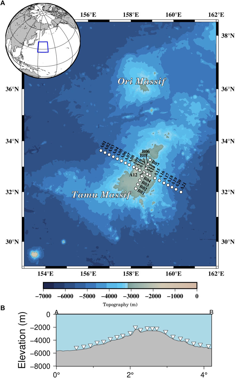
FIGURE 1. (A) Topography of Shatsky Rise and the distribution of OBSs. The blue box in the top left corner of the small map shows the research region. Shatsky Rise is located on the eastern side of the Japan Island and Japan Trench, and the inset shows the location of Shatsky Rise relative to the northwest Pacific Ocean and the main features, such as Tamu Massif and the Ori Massif. Tamu Massif is the largest single volcano on Earth as mentioned in the article, and is the main research region. The white circles are submarine seismographs. (B) Topographic profile of OBS on the Tamu Massif for survey line (A). The white triangle on the top figure represents the OBS.

The largest and oldest edifices in Shatsky Rise, Tamu Massif, which is regarded as the largest single volcano on Earth, was formed in the late Jurassic period (∼147–145 Ma) and is located southwest of Shatsky Rise (Sager et al., 1988). The summit of Tamu Massif is at a depth of 2 km underwater, with a height of about 4 km high and an area of about 3 × 10⁵ km², making it the largest single volcano on Earth, comparable in size to the largest volcano in the Solar System, Olympus Mons on Mars (Sager et al., 2013). Paleomagnetic analysis of cores and borehole logging reveals that it was formed near the equator and then drifted to the present high-latitude location through long-term plate movement and plate drift (Tominaga, 2012; Nakanishi et al., 2015). The majority of the magnetic anomaly at this location illustrates a linear distribution with a trend from southwest to northeast, which is consistent with the volcano’s main axis (Sager et al., 2019). The existence of enormous thick lava flows in Tamu Massif, similar to the lava flows found in the Ontong Java Plateau and continental flow basalts, suggests that Tamu Massif may have been formed by a huge number of basaltic magma eruptions (Sager et al., 2013). Additionally, the drill holes at this location also indicate that the lava flows are mainly composed of interbedded massive lava flows and pillow lava flows (Sager et al., 2010). The seismic profiles obtained from multi-channel seismic (MCS) surveys reveal that Tamu Massif has only one crater and is a giant monolithic, shield-shaped volcano with a maximum 650 km width circular dome, a relatively flat top, and gentle slopes and low angles (0.5°∼1.5°) on the flanks (Sager et al., 2013). Only the middle part of the summit area has a thicker sediment layer and the thickness of the sediment layer becomes progressively thinner as approaches the outer edges on both sides, generally less than 300 m (Sliter and Brown, 1993).

Tamu Massif is far from the mainland and submerged in water, making it more challenging than on land to collect geological and geophysical data. Additionally, due to the limitations of the data collection instruments, the quality of the data is not comparable to that of data collected on land. Despite the limitations of various objective conditions, there are still many studies of the region, and the results provide much understanding of it. Some scholars have proposed the hypothesis of mantle plume model of oceanic plateau by the relative volumes of melt and eruption rates of flood basalts and hot spots as well as their temporal and spatial relations or plate rotations in the hotspot reference frame (Richards et al., 1989; Duncan and Richards, 1991). Some other scholars have proposed that the oceanic plateau formed in the mid-ocean ridge model through seismic tomography, petrographic experiments, or magnetic anomaly map constraints (Anderson et al., 1992; Anderson, 2001; Foulger, 2007; Sager et al., 2019; Huang et al., 2020). At the location of Pacific-Farallon-Izanagi triple junction, many scholars provide support for the hypothesis of the mantle plume-mid-ocean ridge model through the investigation of magnetic anomaly strips, logging data from the IODP, and the proposal of a new method to estimate the eruption rate (Sager et al., 1988; Sager and Han, 1993; Nakanishi et al., 1999; Luo et al., 2019; Zhang et al., 2020).

In this paper, we focuses on Tamu Massif, within Shatsky Rise—the third largest oceanic plateau on Earth, to constrain the oceanic crustal structure by autocorrelating the teleseismic P-wave coda record collected by the hydrophone component of the OBSs. We hope these results can provide some new implications for the research of Shatsky Rise formation mechanism.

2 Data and method

2.1 Teleseismic data

The teleseismic data provided in this study obtained from the IRIS global network, these data were recorded at a total of 28 broadband OBSs deployed on Tamu Massif of Shatsky Rise by the Woods Hole Oceanography Institution (WHOI). Our data consists of the teleseismic events recorded by the hydrophone component of each station between July and September 2010, all the earthquake events used in the study are based on the earthquake catalog published by the United States Geological Survey (USGS), and these event were selected with the following criteria: (a) earthquakes with M_w ≥ 4.8; (b) epicenter distance between 30° and 90°. We excluded earthquakes with epicenter distances less than 30° in order to keep the near-vertical incidence of P-wave. Earthquakes with epicenter distances between 90° and 120° were excluded due to the ray paths of these events bypass at the core-mantle boundary and being sensitive to the core. After selected, we have obtained a data set with raw hydrophone component records of a total of 155 seismic events (Figure 2; Supplementary Table S1).

FIGURE 2

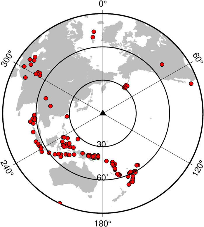
FIGURE 2. Distribution of seismic event. The black triangles in the figure indicate the location of the station network deployed in the research region; the red dots indicate the location of the seismic events selected in the study.

The hydrophone component of the OBS was chosen for this study for two reasons. First, if the OBSs are poorly coupled to the substrate when deployed on the soft seafloor sediments, resulting in low signal-to-noise ratios of the recorded three-component signals, particularly the horizontal component recordings, makes it difficult to apply the receiver function which uses passive source data, although it has been widely used in the detection of continental lithospheric discontinuities. While the hydrophone component of OBS is suspended in water and is not affected by the coupling condition, the signal-to-noise ratio of the recorded signal thus is higher than the three-component signals and provides more useful information. Second, compared with the traditional component, uses the hydrophone component alone for autocorrelation calculation, reducing the step of rotating the component in the conventional seismic method, it alleviates the difficulty of usage and simplifies the processing steps. In this study, a total of 28 broadband OBSs were deployed along two survey lines across Tamu Massif (Figure 1). Line A extends through the entire Tamu Massif from west to east, while line B extends from south to north, covering the central part of the volcano. The distribution of these two lines allows us to obtain the structural changes information of the oceanic crust in the different directions of Tamu Massif. The thin sediment beneath most of the stations has less influence on the arrival of the reflection signal, ensuring the accuracy of the results.

2.2 Method

In this study, we apply a novel geophysical method proposed by Dong et al. (2022) to calculate the autocorrelation of the teleseismic P-wave coda recorded in the hydrophone component of OBSs. P-wave coda is the oscillations of the ground continuing long after the slowest theoretical primary wave arrival time, this part corresponds to the recorder energy after the passage of all primary waves. Since the previous studies, it has been clearly proven that coda waves are an effective resource in extracting information about the characteristics of wave paths, it contains a great deal of information from underground (Herraiz and Espinosa, 1987). Based on the characteristics of the P-wave coda, we can calculate its autocorrelation to detect the lithospheric discontinuities.

After obtaining the original waveform records, we convert the original format to SAC format, and rewrite the channel header information. Then, we remove some non-zero values and linear trends of the data, which are caused by the nature of the instrument, in order to preserve the calculation and analysis of the data. In the following step, we select a window around the theoretical primary wave arrival time in seismogram, the window length is a generic parameter adapted to a particular type of application (Phạm and Tkalčić, 2017). We used the AK135 global velocity model (Kennett et al., 1995) to calculate the theoretical arrival times of P-waves for different seismic events, and intercepted waveforms 5 s before and 45 s after the theoretical arrival time of the selected seismic events, this window length containing the P-wave coda data required for our study, the multiple reflection signals from the lithospheric discontinuity surface and reflections from the deeper lithosphere. Meanwhile, we use Hanning windows to taper off both ends of the waveform to avoid spectral domain artifacts during the time domain to frequency domain conversion and calculation.

Due to Earth filtering, high-frequency signals are quickly absorbed and attenuated by geodesic filtering and low-frequency signals become dominant. To address the problem of low-frequency bias in the records, we adopted spectral whitening to amplify the high-frequency signal content while reducing the low-frequency signal content. The variation of the width of the spectral whitening window we set affects the distribution and energy of the illusion only and does not interfere with the signal from the reflecting interface, thus not affecting our identification of the real signal. Finally, we use a zero-phase band-pass filter of 0.5–3 Hz to improve the sharpness of the reflection signal (by removing the very long period signals) and to avoid spurious effects caused by the unexpected amplification of very high frequency noise due to the spectral whitening.

We compute the autocorrelation of the whitened waveform in the time domain, and retain a half of the symmetric autocorrelogram having positive time lags. After calculating the P-wave coda autocorrelation, we normalize autocorrelation results according to the amplitude and then stack the normalized results by linear stacking to improve the signal-to-noise ratio. Then the stacked P-wave coda autocorrelation results of each station are arranged according to projection points to obtain the P-wave coda autocorrelation amplitude curve profile of Tamu Massif. The oceanic crust structure and Moho reflectors beneath the volcano are then identified through the reflected signals on the profile.

3 Synthetic experiment

In this section, we describe synthetic experiments performed to demonstrate the feasibility of the method to recover the crustal structure. In this regard, we perform a synthetic experiment to recover subsurface structural information by synthesizing complete seismograms and autocorrelating the seismograms. For this purpose, we set up a simple three-layer model with the following model parameters: 1) water layer of 4.5 km thickness, P wave velocity 1.5 km/s, and density 1.0 g/cm³; 2) oceanic crust layer of 6.5 km thickness, P wave velocity 6.5 km/s, and density 2.8 g/cm³; 3) mantle layer of 4.5 km thickness, P wave velocity 8.1 km/s, and density 3.3 g/cm³. Afterwards, an earthquake source was added in the mantle layer. The experiments are designed to synthesize complete seismograms recorded for a receiver on top of a horizontally stratified media bounded by a free surface. The synthesis experiment is to verify the feasibility that moho can be recovered from the reflected signal after autocorrelation. The setting of these values is mainly based on the widely previous studies.

Figure 3A shows the synthesized waveform of the three-layer model. The synthesized waveform is processed and the autocorrelation is calculated by the steps we mentioned above to obtain the autocorrelation synthesis of the synthesized waveform (Figure 3B). In order to avoid difficulties in interpretation caused by high-order multiple waveforms, the correlation time window length is 10 s, and the autocorrelation is symmetric about the moment 0, while there is a maximum peak inherent in the autocorrelation at the moment 0, which can be seen as the teleseismic direct P-wave signal. In Figure 3B, the primary Moho reflection signal at 2 s is p_mp, the secondary Moho reflection signal at 4 s is 2p_mp, the maximum negative amplitude signal at 6 s is the primary water surface reflection signal (p_wp), and the p_mpp_wp signal at 8 s is the primary Moho reflection followed by the primary water surface reflection. The autocorrelation results show that the method can accurately extract the arrival and polarity information of the stratigraphic signals. Subsequently, we modified the model parameters to the layer composed of massive basalt and pillow basalt and the lower oceanic crust, the similar autocorrelation synthetic waveforms can be obtained, and the synthetic experiment illustrates the feasibility of P-wave coda autocorrelation for oceanic crust structure recovery.

FIGURE 3

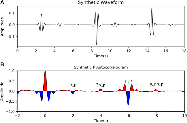
FIGURE 3. (A) Synthetic waveform diagram of the three-layer simple model. The diagram contains direct P-wave, water, primary Moho reflection Pp_mp, and more complex multiple reflections. (B) Autocorrelation of synthetic waveforms. This diagram contains the primary reflection signals of water p_wp and Moho p_mp and secondary reflection signals of Moho 2p_mp.

4 Results

A total of 28 broadband OBSs were employed, and 16 stations recorded reflection signals from the internal oceanic crust, showing at least two clear signal peaks. As for the results of the remaining stations, either only the reflected signal from the water surface can be identified or the autocorrelation results show noise patterns. These results give no useful information, thus not being discussed in the following. In this paper, we have shown the station A16 (Figure 4) with only two reflected signals, and the stations A01 (Figure 5) and A07 (Figure 6) with more than two reflected signals.

FIGURE 4

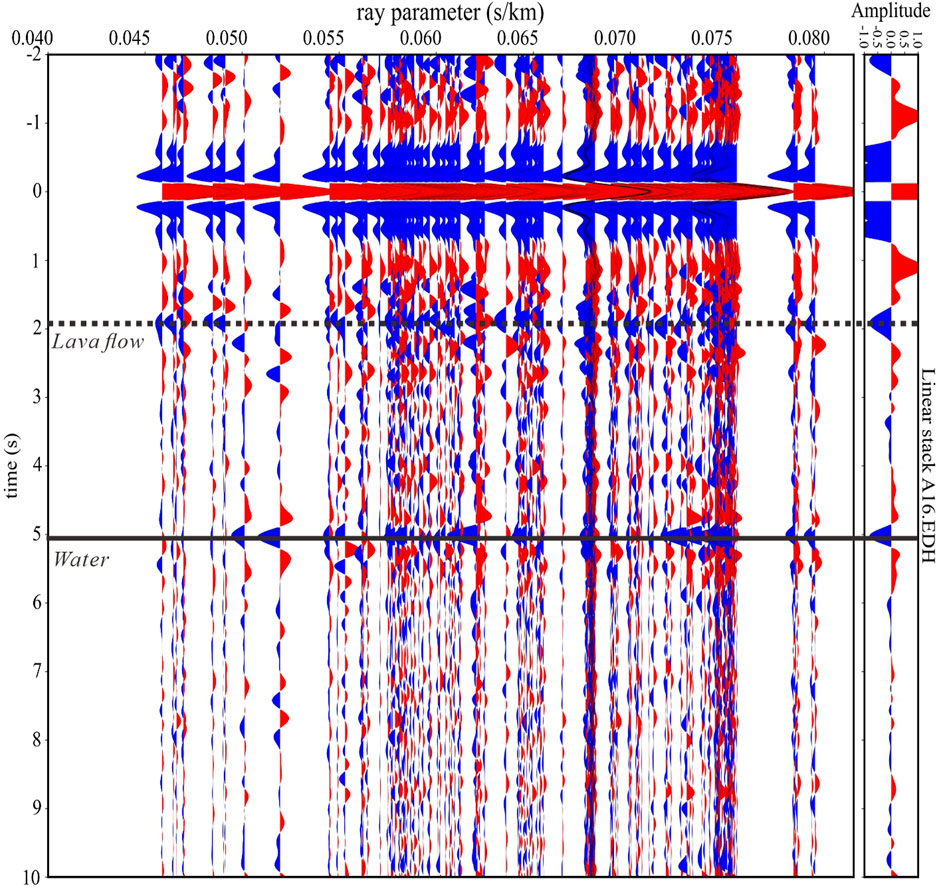
FIGURE 4. P-wave coda autocorrelation results for station A16. Autocorrelation results of the ray parameters of station A16 and the stacking results. The solid black line indicates the reflection signal at the water surface, and the dashed black line indicates the reflection signal at the alternating lava flow.

FIGURE 5

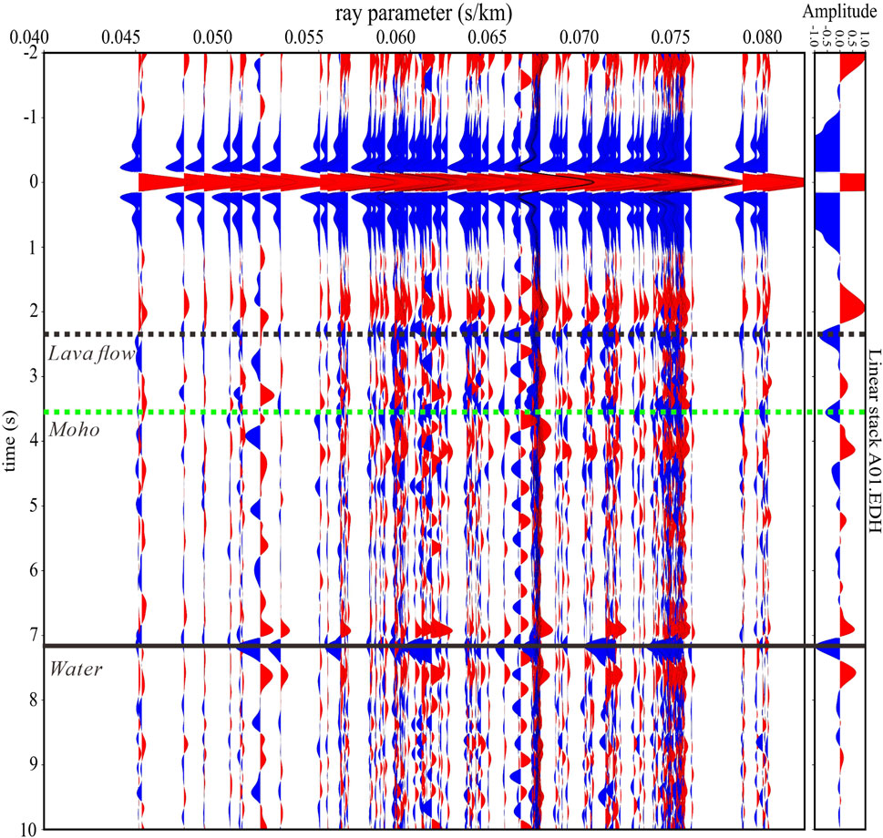
FIGURE 5. P-wave coda autocorrelation results for station A01. The large rectangular box shows the autocorrelation results arranged by ray parameters, and the small vertical rectangular box on the right shows the results after stacks by ray parameters. The black dashed line indicates the lava flow reflection signal, the green dashed line indicates the Moho surface reflection signal, and the black solid line indicates the water surface reflection signal.

FIGURE 6

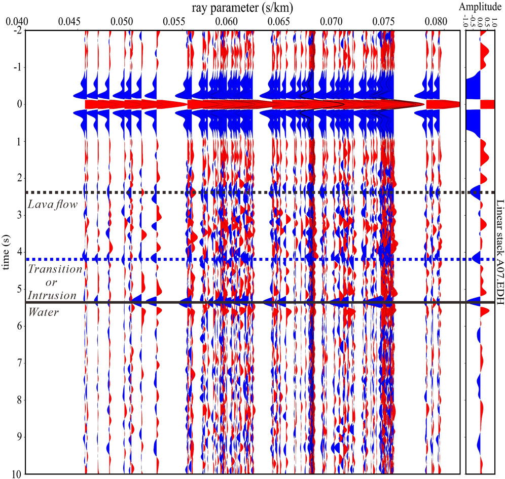
FIGURE 6. P-wave coda autocorrelation results for station A07. The blue dashed line indicates a reflected signal that may be the transition from the upper crust to the lower crust, or a reflection caused by the intrusion within the lower crust.

4.1 Tamu Massif oceanic crust structure

For the results with only two signal peaks, we first exclude the reflected signals from the water surface, then identify the reflected signals from the oceanic crust and characterize these signals to depict an overview of the structure of the oceanic crust beneath the Tamu massif. Taking station A16 as an example (Figure 4), this station is located on the flanks slope of Tamu Massif, where the water depth is quite deep and the wave propagation time in the water is relatively long. We arrange the autocorrelation results for different seismic events according to the ray parameter, which indicates the unique horizontal slowness corresponding to each earthquake event, then identify structure information by recognizing reflected signals on the ray parameters. In the autocorrelation results for station A16, the signal reflected from the water surface is clearly separated from the signal reflected, which from the oceanic crust by stacking the autocorrelation results for each ray parameter, thus two signals can be easily distinguished from each other. The water depth of station A01 is 3,755 m and the wave propagation speed in water is 1.5 km/s, thus the theoretical two-way travel time of the reflected signal from the water surface should be at about 5.00 s. The polarity should be negative after the reflection from the water surface (Dong et al., 2022). In Figure 4, we can see an obvious negative phase with a two-way travel time of about 5.0 s, which is consistent with the theoretical characteristics of the water surface reflection signal, so we identify it as the reflection signal from the water surface. In analogy, the two-way travel time of the water surface reflections can be calculated based on the deployment depth of each OBS in the cruise record of Korenaga and sager (2010). Combining with the polarity of phases, we can distinguish two signals that are close in time, thus other reflection signals could be analyzed more accurately. In Figure 4, it can be seen that after linear stacking of the results, another reflection signal is present at ∼2.0 s, which indicates the presence of a reflection interface at this depth, and this interface is observed in several ray parameters.

Different with Figures 5, 6, the two-way travel times of the reflection signals from the internal structure of oceanic crust is not consistent in different ray parameters generally distribute in 1.8∼2.2 s (Figure 4). After stacking, it can be identified that the depth of the structure reflector is located at the two-way travel time of ∼1.9 s beneath the Tamu massif. Autocorrelation results for most of the OBS stations at the Tamu Massif show a similar pattern, that is the reflected signals recorded on different ray parameters are scattered. On the contrary, station A01 (Figure 5) and A07 (Figure 6), demonstrate that the times of reflection signals from internal structures in the oceanic crust are relatively consistent at most ray parameter. The reflection signals from this structure are seen at the two-way travel time of ∼2.4 s and can be identified without stacking. In the profile of line A, reflected signals from internal oceanic crust structure can be seen in the stacked autocorrelation results of most stations. These signals vary in depth, they are all located at 1.5–2.5 s (Figure 7) and are generally parallel to the terrain.

FIGURE 7

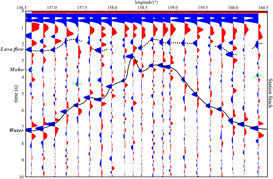
FIGURE 7. The OBS autocorrelation result profile of the A line of Tamu Massif. The stations arranged from left to right according to their actual positions projected onto the profile. The solid black line shows the water surface reflection signal, the dashed black line shows the lava flow reflection signal, and the dashed green line shows the Moho surface reflection signal.

We consider this signal as reflections from a layer composed of alternating eruptions of denser, higher velocity massive lava and sparser, lower velocity pillow lava flows, which have less density and lower velocity compared to the lower oceanic crust, with a strong acoustic impedance contrasts between them and thus able to generate a reflection signal.

4.2 Seismic Moho under Tamu Massif

On the profile, except for the reflection signals of the layer composed of lava flows and the water surface, some stations have also recorded a signal from other reflectors. Taking stacked autocorrelation results of station A01 as an example (Figure 5), there is a reflection signal at 3.6 s that has not yet been recognized, in addition to the reflection signals from the water surface at 7.2 s and the lava flow at 2.3 s. This reflection signal has the same characteristics as the two identified reflections in the autocorrelation results, with a clear amplitude at the two-way travel time. In addition, the signal keeps clear when adapting different widths of the Hanning window or bandpass range, indicating an interface at the corresponding depth. After distinguishing the reflection signals received by these stations from this interface and projecting them on the line A profile of Tamu Massif (Figure 7), it can be seen that the interface is situated a few seconds beneath the Tamu Massif on both sides and deepen overall as it approaches the middle. Signals from these reflectors are seen at about 3.6 s below station A01, at about 4.5 s below station A05, at about 3.7 s for A21 (Figure 7), while these reflectors are not observed at the remaining stations. This suggests that this interface is not quite continuous or the interface is too weak to produce a consistent reflective signal.

For those signals with two-way travel times >2.5 s, we consider them to be reflections from the Moho. Similar to the receiver function, probably because the energy of the secondary Moho is faint and weaker than the noise energy, the reflection signal of 2p_mp is invisible in results, thus we focus on identifying the signals from the primary reflection phase of the Moho. The results are agreement with previous results obtained from various geophysical methods (Sager et al., 2010; Korenaga and Sager, 2012; Zhang et al., 2015; Zhang et al., 2016; Chen et al., 2022), that is, the Moho reflectors move from shallow to deep from the sides toward the middle, the thickness of the oceanic crust becomes thicker (Figure 7). Because of the thick crust in the middle of the volcano, it is difficult to receive the reflected signals from the Moho reflectors in the middle part.

5 Discussion

5.1 Sources of the receiver signals

Before recognizing the received signal’s the source, we took steps to confirm the signal’s reliability, ensuring that the signal we analyze in the discussion following is a true reflected signal. To ensure that our target signal is preserved as much as possible and to minimize interference from other frequency signals, filtering is a crucial step in this work. Our expected detection range is the lithosphere, and at the beginning of the study, because the bandpass filter was set too low, the reflection signals from deeper depths were mixed with the expected signals, making it impossible to distinguish and identify the signals useful for this study. When the bandpass filter was set too high, there were too many high frequency signals that contain information that is not useful to us, and we could not identify which was the expected signal. After extensive testing, we set the bandpass filtering in the range of 0.5∼3.0 hz. Within that bandwidth, the reflected signal from the oceanic crustal structure beneath Tamu massif is most prominent. We also adjusted the window of spectral whitening and the length of the cut time window of the received signal, and can see that the waveform of the real reflected signal does not change after doing these operations, so we can confirm which are the valid signals in the autocorrelation results.

We propose that the reflection signal 1.5–2.5 s below the sea floor of Tamu Massif is from a layer composed of alternating eruptions of denser, higher velocity massive lava and sparser, lower velocity pillow lava flows, which have less density and lower velocity compared to the lower oceanic crust, judged mainly in combination with previous Integrated Ocean Drilling Program (IODP) core and borehole logging data (Sager et al., 2011), MCS profiles interpreted by synthetic seismogram for IODP (Sager et al., 2013; Zhang et al., 2015; Zhang et al., 2016), OBS refraction signals (Korenaga and Sager, 2012). Evidence from synthetic seismograms of core and borehole logging data from ocean drilling suggests that the basement of Tamu Massif is dominated by dense massive lava flows with pillow lava flows interspersed (Sager et al., 2013), with similar features beneath the basement of some other oceanic plateaus such as the Ontong Java Plateau, the Manihiki Plateau and Kergulen Plateau (Rotsein, 1992; Rotstein et al., 1992; Inoue et al., 2008; Spitzer et al., 2008; Pietsch and Uenzelmann, 2015). Results from IODP and synthetic seismograms show that massive lava flows interstratify with pillow lava flows above the oceanic crust of the Tamu Massif, supporting the possibility that the upper oceanic crust portion of the Tamu Massif can constitute a mixed layer of massive and pillow lava flows. The velocity structure provided by the OBS refraction also demonstrates that the seismic wave velocity above the oceanic crust is low and increases with depth, and eventually has a significant difference with the seismic wave velocity in the middle of the oceanic crust, and we find the interface of the seismic wave velocity discontinuity that may be caused by this layer through the teleseismic P-wave coda autocorrelation. The depth of this layer can be seen at about 1.5–2.5 s of two-way travel time beneath the sea floor. They are generally parallel to the seafloor terrain, may suggesting that they may formed during rapid eruptions of viscous low magma.

After identifying the reflection signals from the water surface and lava flows in the autocorrelation results, reflection signals from other interfaces deeper below the sea floor can be identified consequently. Reflection signals indicate a discontinuous interface distributed on both sides of Tamu Massif and the interface signal gradually disappears as moves toward the middle of the volcano. The energy and the quality of the interface reflected signal varies in stations, with some stations receiving clear signals and some slightly blurred, for which we infer that the signal comes from the Moho reflectors at the crust-mantle boundary. Although there is no independent verification that this reflector is Moho, but we can comparing our results with the oceanic crust models of previous multi-channel seismic surveys and gravity investigation (Korenaga and Sager, 2012; Zhang et al., 2015; Zhang et al., 2016; Chen et al., 2022). We found some stations that the two-way travel time of the signal is consistent with Moho reflectors detected by others, and Moho distribution pattern consistent with the previous observations that oceanic crust grows thicker as it approaches the middle of the volcano (Figure 8). In Figure 8, we project some OBS stations which have observed the Moho to the corresponding location of Zhang et al. (2016) MCS reflection profile and compare with their results, the red dot represents the reflection signal we received from Moho, the projected signal two-way travel time is consistent with the Moho as interpreted by Zhang et al. (2016) based on the multi-channel seismic reflection profile.

FIGURE 8

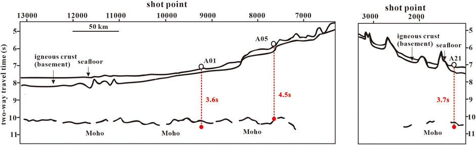
FIGURE 8. Projection of A01, A05, and A21 stations on the multi-channel seismic profile. The white dots represent OBS, the red dot indicates the Moho we identified and projected it on the profile for comparison.

For A07 station, except for the reflection signals from water and lava flows, a signal is shown at 4.2 s (Figure 6). We do not interpret it as Moho because its arrival is shallower than that of A05, which is inconsistent with the gradual deepening trend of Moho as interpreted by previous researchers (Korenaga and Sager, 2012; Zhang et al., 2015; Zhang et al., 2016; Chen et al., 2022). Hence, for the signal that is shallower than Moho, we infer that it may be the transition from the upper crust to the lower crust, or a reflection caused by the intrusion within the lower crust.

5.2 The structure of the oceanic crust

Oceanic plateaus are less studied than continental since they are more difficult to access and submerged under the water, making it difficult for researchers to collect data. Even though it might be challenging to collect data, it is still essential to investigate the oceanic plateau. Scholars have attempted to research the oceanic plateaus from a variety of approaches in order to understand and learn more about the evolutionary formation mechanisms of these plateaus, in Shatsky Rise, there have been some geophysical studies here (Sager et al., 2010; Korenaga and Sager, 2012; Zhang et al., 2015; Zhang et al., 2016; Sager et al., 2019; Huang et al., 2020; Chen et al., 2022). These researches have collected spatial information and stratigraphic structure of the Shatsky Rise region by different geophysical methods. In this paper, teleseismic P-wave coda autocorrelation was applied in this region, and these results provide new constraints on the structure of the oceanic crust beneath the Tamu Massif.

In our autocorrelation results, we have retrieved the structure of the oceanic crust of the Tamu Massif. Within the volcano, a layer composed of denser, higher velocity massive lava and sparser, lower velocity pillow lava flows is found, although this signal has not been identified in active source seismic data (Sager et al., 2010; Zhang et al., 2015; Zhang et al., 2016). We infer that the cause of this situation is the difference in resolution among geophysical methods. Active source seismic using to shorter wave length, the obtained seismic profiles usually have a higher resolution and can obtain the delicate structure of the underground. In contrast, the P-wave of passive sources has a longer wavelength and can reflect a larger range of velocity variations, although at lower resolution. Therefore, we infer that the strata of Massive lava and pillow lava flows in the Tamu Massif are deeper beyond the resolution of MCS profiles, but can be detected by our approach.

Although the two-way travel time of the reflected signals from the water surface shows strong consistency, the two-way travel time of the signals from the internal structure of the oceanic crust shows some variations in some of the autocorrelation results with different ray parameters (Figure 4), and these signals can recover clear reflections after stacking. But in some other stations, there is a high consistency among the autocorrelation results of the signals from the internal structure of the oceanic crust in different ray parameters, such as A07 (Figure 7), those strong and clear lava flow reflection signals can be identified in most of the autocorrelation results of seismic events without linear stacking. We deduce the following two explanations as to why some stations failed to record the interface of alternating lava flows: 1) The eruption process is not stable and homogeneous, the characteristics of the interface thus are not consistent, resulting in some parts of the interface being clearer and some parts being blurred. 2) Due to the short period of time of instrument deployment, the data used in this study might not with sufficient quality to show the reflections.

6 Conclusion

In this paper, we use the autocorrelation of the teleseismic P-wave coda to constraint the structure of the oceanic crust of Tamu Massif. By extracting and calculating the autocorrelation recorded by 28 OBS hydrophone components, we provide a new finding on the structure of the oceanic crust for Tamu Massif. In our results, a layer composed of alternating eruptions of denser, higher velocity massive lava and sparse, lower velocity pillow lava flows were identified. The layer can be seen from left to right below the sea floor. As the largest and oldest single volcano in the Shatsky Rise, the structure of the oceanic crust of Tamu Massif provides implications for the structure of the oceanic crust of others massif of the Shatsky Rise, and it is expected that the application of this method can be continued on other oceanic plateaus to deepen the knowledge and understanding of the structure of the oceanic crust of large volcanoes on the global seafloor.

Data availability statement

Publicly available datasets were analyzed in this study. This data can be found here: http://ds.iris.edu/mda/.

Author contributions

FX contributed to the data analysis and wrote the original draft of the paper. SL contributed to the conceptualization and supervision. CC and HC helped with supervision and suggestions. SD contributed to the methodology. All authors contributed to the article and approved the submitted version.

Funding

This study is partially funded by the National Natural Science Foundation of China (Grant No. 42074123) and the Pearl River Talent Program of Guangdong, China (Grant No. 2017ZT07Z066).

Acknowledgments

We are grateful to the reviewers and the editor-in-chief for reviewing this manuscript.

Conflict of interest

The authors declare that the research was conducted in the absence of any commercial or financial relationships that could be construed as a potential conflict of interest.

Publisher’s note

All claims expressed in this article are solely those of the authors and do not necessarily represent those of their affiliated organizations, or those of the publisher, the editors and the reviewers. Any product that may be evaluated in this article, or claim that may be made by its manufacturer, is not guaranteed or endorsed by the publisher.

Supplementary material

The Supplementary Material for this article can be found online at: https://www.frontiersin.org/articles/10.3389/feart.2023.1218576/full#supplementary-material

References

Anderson, D. L., Tanimoto, T., and Zhang, Y. (1992). Plate tectonics and hotspots: The third dimension. Science 256, 1645–1651. doi:10.1126/science.256.5064.1645

PubMed Abstract | CrossRef Full Text | Google Scholar

Anderson, D. L. (2001). Top-down tectonics? Science 293, 2016–2018. doi:10.1126/science.1065448

PubMed Abstract | CrossRef Full Text | Google Scholar

Chen, W., Hu, M., Zhang, J., Lin, J., and Zhang, X. (2022). Gravity admittance analysis and its implications for the formation of Tamu Massif in the west Pacific Ocean. Periodical Ocean Univ. China 52, 40–49. doi:10.16441/j.cnki.hd-xb.20220219

CrossRef Full Text | Google Scholar

Coffin, M. F., and Eldholm, O. (1994). Large igneous provinces: Crustal structure, dimensions, and external consequences. Rev. Geophys. 32, 1. doi:10.1029/93RG02508

CrossRef Full Text | Google Scholar

Dong, S., Cai, C., Lu, S., and Zhang, S. (2022). A method and device for acquiring discontinuous oceanic lithosphere information

Google Scholar

Duncan, R. A., and Richards, M. A. (1991). Hotspots, mantle plumes, flood basalts, and true polar wander. Rev. Geophys. 29, 31. doi:10.1029/90RG02372

CrossRef Full Text | Google Scholar

Foulger, G. R. (2007). The “plate” model for the genesis of melting anomalies. Plates, Plumes Planet. Process. 430, 1–28. doi:10.1130/2007.2430(01)

CrossRef Full Text | Google Scholar

Harris, P. T., Macmillan-Lawler, M., Rupp, J., and Baker, E. K. (2014). Geomorphology of the oceans. Mar. Geol. 352, 4–24. doi:10.1016/j.margeo.2014.01.011

CrossRef Full Text | Google Scholar

Herraiz, M., and Espinosa, A, F. (1987). Coda waves: A review. Pure Appl. Geophys. 125, 499–577. doi:10.1007/BF00879572

CrossRef Full Text | Google Scholar

Huang, Y., Sager, W. W., Zhang, J., Tominaga, M., Greene, J., and Nakanishi, M. (2021). Magnetic anomaly map of Shatsky Rise and its implications for Oceanic Plateau formation. J. Geophys. Res. Solid Earth 126. doi:10.1029/2019JB019116

CrossRef Full Text | Google Scholar

Inoue, H., Coffin, M. F., Nakamura, Y., Mochizuki, K., and Kroenke, L. W. (2008). Intrabasement reflections of the Ontong Java Plateau: Implications for plateau construction: Ontong Java Plateau construction. Geochem. Geophys. Geosyst. 9. doi:10.1029/2007gc001780

CrossRef Full Text | Google Scholar

Kennett, B, L., Engdahl, E, R., and Buland, R., (1995). Constraints on seismic velocities in the Earth from traveltime. Geophys. J. Int. 122 (1), 108–124. doi:10.1111/j.1365-246X.1995.tb03540.x

CrossRef Full Text | Google Scholar

Korenaga, J., and Sager, W. W. (2010). Geophysical constrains on mechanisms of ocean plateau formation from Shatsky Rise, Northwest Pacific. MGL1004 cruise report, 1–111.

Google Scholar

Korenaga, J., and Sager, W. W. (2012). Seismic tomography of Shatsky Rise by adaptive importance sampling: Shatsky rise crustal structure. J. Geophys. Res. 117. doi:10.1029/2012JB009248

CrossRef Full Text | Google Scholar

Luo, Y., Zhang, J., and Lin, J. (2019). Recent research advances on Tamu Massif in the Pacific Ocean and implications for the formation of arge oceanic volcanoes. Prog. Geopyhsics 34 (2), 0781–0795. doi:10.6038/pg2019CC-0380

CrossRef Full Text | Google Scholar

Nakanishi, M., Sager, W. W., and Klaus, A. (1999). Magnetic lineations within Shatsky Rise, northwest Pacific Ocean: Implications for hot spot-triple junction interaction and oceanic plateau formation. J. Geophys. Res. Solid Earth 104 (B4), 7539–7556. doi:10.1029/1999jb900002

CrossRef Full Text | Google Scholar

Nakanishi, M., Sager, W. W., and Korenaga, J. (2015). Reorganization of the pacific-izanagi-farallon triple junction in the late jurassic: Tectonic events before the formation of the Shatsky Rise. Special Paper of the Geological Society of America 511, 85–101. doi:10.1130/2015.2511(05)

CrossRef Full Text | Google Scholar

Phạm, T, S., and Tkalčić, H. (2017). On the feasibility and use of teleseismic P wave coda autocorrelation for mapping shallow seismic discontinuities. J. Geophys. Res. Solid Earth 122 (5), 3776–3791. doi:10.1002/2017JB013975

CrossRef Full Text | Google Scholar

Pietsch, R., and Uenzelmann-Neben, G. (2015). The Manihiki Plateau-A multistage volcanic emplacement history: Emplacement of the Manihiki Plateau. Geochem. Geophys. Geosyst. 16, 2480–2498. doi:10.1002/2015GC005852

CrossRef Full Text | Google Scholar

Richards, M. A., Duncan, R. A., and Courtillot, V. E. (1989). Flood basalts and hot-spot tracks: Plume heads and tails. Science 246, 103–107. doi:10.1126/science.246.4926.103

PubMed Abstract | CrossRef Full Text | Google Scholar

Rotstein, Y., Schlich, R., Munschy, M., and Coffin, M. F. (1992). Structure and tectonic history of the Southern Kerguelen Plateau (Indian Ocean) deduced from seismic reflection data. Tectonics 11, 1332–1347. doi:10.1029/91TC02909

CrossRef Full Text | Google Scholar

Sager, W. W., and Han, H. (1993). Rapid formation of the Shatsky Rise oceanic plateau inferred from its magnetic anomaly. Lett. Nat. 364, 610–613. doi:10.10-38/364610a0

CrossRef Full Text | Google Scholar

Sager, W. W., Handschumacher, D. W., Hilde, T. W. C., and Bracey, D. R. (1988). Tectonic evolution of the northern Pacific plate and pacific-farallon Izanagi triple junction in the late jurassic and early cretaceous (M21-M10). Tectonophysics 155, 345–364. doi:10.1016/0040-1951(88)90274-0

CrossRef Full Text | Google Scholar

Sager, W. W., Huang, Y., Tominaga, M., Greene, J. A., Nakanishi, M., and Zhang, J. (2019). Oceanic plateau formation by seafloor spreading implied by Tamu Massif magnetic anomalies. Nat. Geosci. 12, 661–666. doi:10.1038/s41561-019-0390-y

CrossRef Full Text | Google Scholar

Sager, W. W., Kim, J., Klaus, A., Nakanishi, M., and Khankishieva, L. M. (1999). Bathymetry of Shatsky Rise, northwest Pacific Ocean: Implications for ocean plateau development at a triple junction. J. Geophys. Res. Solid Earth 104 (B4), 7557–7576. doi:10.1029/1998jb900009

CrossRef Full Text | Google Scholar

Sager, W. W., Sano, T., and Geldmacher, J. (2011). IODP expedition 324: Ocean drilling at Shatsky Rise gives clues about Oceanic Plateau formation. Sci. Rep. 12, 24–31. doi:10.5194/sd-12-24-2011

CrossRef Full Text | Google Scholar

Sager, W. W., Sano, T., and Geldmacher, J. (2010). “Expedition 324 scientists,” in Proceedings of the Integrated Ocean Drilling Program, Texas, USA.324.

Google Scholar

Sager, W. W., Zhang, J., Korenaga, J., Sano, T., Koppers, A. A. P., Widdowson, M., et al. (2013). An immense shield volcano within the Shatsky Rise oceanic plateau, northwest Pacific Ocean. Nat. Geosci. 6, 976–981. doi:10.1038/ngeo1934

CrossRef Full Text | Google Scholar

Sliter, W., and Brown, G. R. (1993). Shatsky rise:seismic startigraphy and sedimentary record of pacific paleoceanography since the early cretaceous. Rro. Ocean. Drill. Program Sci. Result 132, 3–13.

Google Scholar

Spitzer, R., White, R. S., and Christie, P. A. F. (2007). Seismic characterization of basalt flows from the Faroes margin and the Faroe-Shetland basin. Geophys Prospect 56, 21–31. doi:10.1111/j.1365-2478.2007.00666.x

CrossRef Full Text | Google Scholar

Tominaga, M., Evans, H. F., and Iturrino, G. (2012). Equator Crossing of Shatsky Rise? New insights on Shatsky Rise tectonic motion from the downhole magnetic architecture of the uppermost lava sequences at Tamu Massif. Geophys. Res. Lett. 39. doi:10.1029/2012GL052967

CrossRef Full Text | Google Scholar

Zhang, J., Luo, Y., and Chen, J. (2020). Oceanic Plateau formation implied by Ontong Java Plateau, Kerguelen Plateau and Shatsky Rise. Ocean. Coast. Sea Res. 19, 351–360. doi:10.1007/s11802-020-4246-2

CrossRef Full Text | Google Scholar

Zhang, J., Sager, W. W., and Korenaga, J. (2015). Shatsky Rise oceanic plateau structure from two-dimensional multichannel seismic reflection profiles and implications for oceanic plateau formation. Boulder, Colorado, US: Geological Society of America Special Papers, 103–126. doi:10.1130/2015.2511(06)

CrossRef Full Text | Google Scholar

Zhang, J., Sager, W. W., and Korenaga, J. (2016). The seismic Moho structure of Shatsky Rise oceanic plateau, northwest Pacific Ocean. Earth Planet. Sci. Lett. 441, 143–154. doi:10.1016/j.epsl.2016.02.042

CrossRef Full Text | Google Scholar