Analysing the elevation-distributed hydro-climatic regime of the snow covered and glacierised Hunza Basin in the upper Indus

In the high altitude Hindukush Karakoram Himalaya (HKH) mountains, the complex weather system, inaccessible terrain and sparse measurements make the elevation-distributed precipitation and temperature among the most significant unknowns. The elevation-distributed snow and glacier dynamics in the HKH region are also little known, leading to serious concerns about the current and future water availability and management. The Hunza Basin in the HKH region is a scarcely monitored, and snow- and glacier-dominated part of the Upper Indus Basin (UIB). The current study investigates the elevation-distributed hydrological regime in the Hunza Basin. The Distance Distribution Dynamics (DDD) model, with a degree day and an energy balance approach for simulating glacial melt, is forced with precipitation derived from two global datasets (ERA5-Land and JRA-55). The mean annual precipitation for 1997–2010 is estimated as 947 and 1,322 mm by ERA5-Land and JRA-55, respectively. The elevation-distributed precipitation estimates showed that the basin receives more precipitation at lower elevations. The daily river flow is well simulated, with KGE ranging between 0.84 and 0.88 and NSE between 0.80 and 0.82. The flow regime in the basin is dominated by glacier melt (45%–48%), followed by snowmelt (30%–34%) and rainfall (21%–23%). The simulated snow cover area (SCA) is in good agreement with the MODIS satellite-derived SCA. The elevation-distributed glacier melt simulation suggested that the glacial melt is highest at the lower elevations, with a maximum in the elevation 3,218–3,755 masl (14%–21% of total melt). The findings improve the understanding of the local hydrology by providing helpful information about the elevation-distributed meltwater contributions, water balance and hydro-climatic regimes. The simulation showed that the DDD model reproduces the hydrological processes satisfactorily for such a data-scarce basin.

1 Introduction

Precipitation is one of the key drivers of the hydrological cycle, but is also among the significant unknowns at high elevations (Immerzeel et al., 2012; Ragettli and Pellicciotti, 2012). Similar to other mountain basins globally, precipitation is the main uncertainty in the Hindukush Karakoram Himalaya (HKH) region, yet critical for understanding high altitude hydrology (Immerzeel et al., 2012). The relationship between precipitation and elevation in the region is poorly defined due to the area’s remoteness, inaccessible terrain and sparse measurements (Bookhagen and Burbank, 2006; Immerzeel et al., 2015).

In high elevation mountain basins, snow and glaciers significantly contribute to the river flow (Barnett et al., 2005). Snow is an integral part of the climatic system, significantly influencing atmospheric processes because of its low thermal conductivity and high albedo (Hall and Riggs, 2007). The snow and glaciers in the HKH region sustain the freshwater availability in the Himalayan and adjacent plains. Seasonal snow and glaciers from the HKH region provide freshwater in the downstream areas from April-October (Hasson et al., 2014). Meltwater from the HKH region is critical for the irrigation, hydropower production, and drinking water needs of millions of people in Southeast Asia. This meltwater is also associated with high water levels in lakes and reservoirs and subsequent increased risk of downstream flooding (Qureshi et al., 2017). Due to the lack of precipitation data in the Indus Basin, the snow cover area (SCA), snow water equivalent (SWE), and glacier mass balance are not fully known (Bolch, 2017). The current understanding of snow and glacier melt contribution to the Indus runoff is hence based on insufficient analysis and very limited data (Nazeer et al., 2021).

The agro-based economy in Pakistan depends on water supplied from the River Indus and its tributaries for irrigation (Raza et al., 2012). The water for the Indus Basin Irrigation System (IBIS), the largest irrigation system in the world, originates from the HKH region and is regulated by two major reservoirs, i.e., Tarbela on River Indus and Mangla on River Jhelum. The rainfall in the plains of the IBIS is, in general small (<200 mm/year) (Ali et al., 2009), so the upstream snow and glaciers are critical to sustain this irrigation system. The Hunza Basin is one of the main sub-basins of the Upper Indus Basin (UIB). It contributes about 12% of the total flow of the River Indus upstream of the Tarbela reservoir (Shrestha et al., 2015). In the Hunza Basin, the area above 5,000 masl receives maximum snowfall and is considered the most active hydrological zone of the basin (Young, 1985). With only three installed gauges in the basin below 5,000 masl, it is challenging to get realistic precipitation and its spatial distribution (Saroj Shrestha 2019). Moreover, the basin has extensive glaciers (about 30% of its total area) that contribute significantly to the river flow. These glaciers cannot persist unless precipitation in the basin is much higher than what is observed by the existing gauges (Immerzeel et al., 2011).

Different studies (Tahir et al., 2011; Immerzeel et al., 2012; Ragettli and Pellicciotti, 2012; Lutz et al., 2014; Shrestha et al., 2015; Shrestha and Nepal, 2019) used different data (e.g., gauges data with precipitation lapse rates, APHRODITE, virtual weather stations (VWSs), ERA-Interim) to estimate precipitation at high altitudes. The mean observed annual precipitation was 660 mm at Naltar (2,810 masl), 292 mm at Ziarat (3,669 masl) and 165 mm at Khunjrab gauge (4,730 masl) in the Hunza basin from 2000 to 2004 (Shrestha et al., 2015). Since the mean annual flow is 730 mm for the same period (750 mm for 1997–2010) in the Hunza River, it may suggest that these three stations are insufficient to estimate precipitation of the entire basin and/or there is a significant contribution to the runoff from glacier storage. In addition, there appears to be a negative precipitation gradient in the Hunza Basin, with maximum precipitation at lower elevations (Naltar station) and the minimum at higher elevations (Khunjrab station). So, deriving precipitation for higher elevations using simple lapse rates may introduce uncertainty in assessing the hydrological processes.

Models are primarily used for investigating hydrological processes and predicting fluxes. The model that provides accurate results using the least parameters and with the least complexity is ranked as the best (Skaugen and Weltzien, 2016). Various hydrological models with diverse applications, ranging from small catchments to the global scale, have been developed (Skaugen and Weltzien, 2016). Maskey (2022) has reviewed a wide range of catchment hydrological models, which include models that simulate snow accumulation and melt processes. Hydrological models can be classified as lumped, semi-distributed and distributed, on a spatial scale basis. Many approaches have been developed within conceptual and distributed hydrologic modelling frameworks to better represent the snow and glacier processes (Shrestha et al., 2015). These models are, in general hydrological models but also simulate the snow/glacier and hydrological dynamics and associated climate change implications (for example,; SRM (Martinec (1975), DDD (Skaugen and Onof, 2014), SPHY (Terink et al., 2015), GDM (Kayastha and Kayastha, 2020). There are two basic approaches to simulate snow and glacier melt: degree day and energy balance. The degree day approach only uses temperature for melt simulations. The energy balance model considers the overall energy budget of the system for estimating snow and glacier melt. Energy balance-based snow and glacier melt modelling is generally better suited to accurately describe the hydrologic processes (Shrestha et al., 2015). In this study, two versions of the Distance Distribution Dynamics (DDD) model with energy balance (EB) and degree day (DD) based sub routines are used for estimating glacial melt. The former is more physically based and has no parameters to be calibrated, whereas the latter uses the degree-day factor as a calibration parameter. DDD is a hydrological model specially designed for snow and glaciers dominated catchments and is applied in Norway (Skaugen and Onof, 2014). More details about this model are discussed in Section 2.3. In the earlier research by Nazeer et al. (2021), the DDD model was applied in the Gilgit Basin (another sub basin of the UIB), and showed its potential for reasonably simulating the hydrological regime of the UIB.

Many recent attempts have been made to simulate the hydrological regime of the Hunza Basin/Upper Indus Basin/Hindukush Karakoram Himalaya region using a variety of input data and modelling approaches. Tahir et al. (2011) applied the snowmelt runoff model (SRM) coupled with MODIS snow cover data to simulate the Hunza’s daily flow under climate change scenarios. They concluded that new reservoirs are required to meet future water needs (e.g., irrigation, hydropower generation, and drinking water supply) and flood control. Mukhopadhyay and Khan (2014) estimated flow for the UIB and concluded there would be long-term reductions in river flows under climate change. Mukhopadhyay and Khan (2015) concluded that glacier melt contribution is higher than snowmelt in the rivers of the Karakoram. Hasson et al. (2014) suggested a decreasing annual snow trend for the westerlies-influenced sub-basins and an increasing trend for the monsoon-influenced sub-basins of the Indus.

This study complements the earlier studies in the data-scarce Hunza Basin in the following ways: i) simulating the elevation-distributed hydro-climatic dynamics (in particular snow and glacier melt runoff and rainfall runoff from 10 different elevation zones) using a comparatively new modelling approach which was tested in river basins in Norway (Skaugen and Onof, 2014), ii) comparing snow and glacier melt simulations from the energy balance (EB) and degree day (DD) approaches, and iii) quantifying the components of runoff and the water balance for the Hunza Basin. So the overarching objective of this study is to analyse the elevation-distributed SCA, snow and glacier melt (GM), SWE, flow simulations and water balance of the Hunza Basin. This will increase the understanding of the flow regime and hydrological processes of such a scarcely monitored, high altitude glaciated and snow-fed basin.

2 Materials and methods

2.1 Study area

The Hunza Basin (13,713 km²) extends from 74.04 to 75.77°E and 36.05–37.08°N and is located in the Karakoram mountains of the HKH region (Figure 1). About 80% of the total flow into Tarbela reservoir originates from the snow covered and glaciated parts, which is less than 20% of the total basin area of the Indus (Archer and Fowler, 2004). The Hunza Basin is a high altitude (1,425–7,889 masl) basin with a mean elevation of 4,600 m (Table 1; Supplementary Figure S1). The basin has a dense river network with the Hunza River as the main tributary (232 km long) and Shimshal, Verjerab, Hispar, Hoper, Naltar Rakaposhi, Khunjrab and a few others as minor tributaries (Garee et al., 2017). The 1966–2010 flow data recorded at the Danyore gauge (the outlet of Hunza River) by the Water and Power Development Authority (WAPDA) of Pakistan shows an average flow of 304 m³/sec (∼710 mm/year). The Hunza River has minimum flow during the snow accumulation seasons (Nov to early April). Flow increases with temperature and reaches a maximum in July/August (Shrestha et al., 2015). The climate in the Hunza Basin is arid to semiarid and divided into four seasons; winter (Dec-Feb), spring (March-May), monsoon (June-Sep), and post-monsoon season (Oct-Nov) (Nazeer et al., 2021). The HKH region has two primary sources of precipitation; summer monsoon and winter westerlies. The Hunza Basin receives precipitation from both sources, although the winter westerlies contribute about two-thirds of the total precipitation (Bookhagen and Burbank, 2010). At the seasonal snow maximum in winter, almost 85% of the total area is covered with snow (Shrestha et al., 2015). The glacier coverage is about 30% of the total area and is found between 2,300 and 7,889 masl [RGI v6.0 (Arendt et al., 2017),]. The basin hosts extensive glacier systems, including Hispar (339 km²), Batura (238 km²), Virjerab (112 km²), Khurdopin (111 km²) and a few others.

FIGURE 1

FIGURE 1. Location of the study area, glacier cover, river network and meteorological stations.

TABLE 1

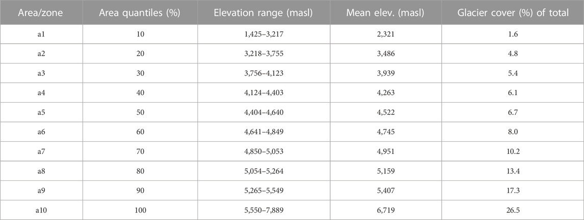
TABLE 1. Hypsometry of the Hunza Basin (divided into ten elevation bands of equal area) and glacier cover (Source: SRTM 30 m DEM & RGI 6.0).

2.2 Data

The Hunza Basin has three meteorological stations (Naltar 2,810 masl, Ziarat 3,669 masl, Khunjrab 4,730 masl) installed and managed by WAPDA. The meteorological stations record daily temperature and total precipitation. The mean temperature and precipitation data from 1997 to 2010 are used in the current study. The Naltar and Ziarat stations record monthly maximum precipitation in April and minimum in November. The Khunjrab station records monthly maximum precipitation in August and minimum in October. The Naltar station records maximum annual precipitation of 701 mm, and the Khunjrab station recorded a minimum of 190 mm (average values from the 1997–2010 data).

The annual average temperature is 6.6°C, 3.0°C and −5.01°C at Naltar, Ziarat and Khunjrab stations respectively. The monthly mean temperature is maximum in July and minimum in January at all stations. The flow gauge of the Hunza Basin is installed at Danyore Bridge (1,456 masl). The Hunza River has a low flow period from October to March and a high flow period from April to September. The high flow period is further divided into snowmelt dominated (April to June) and glacier melt dominated (late June to September) periods (Hasson, 2016).

The European reanalysis 5 Land (ERA5) data (Table 2) (Muñoz Sabater, 2019) were used to derive elevation-distributed precipitation for the Hunza Basin from 1997 to 2010 due to their good performance assessed through hydrological modelling by Nazeer et al. (2021) and their high resolution. The dataset is freely available at https://cds.climate.copernicus.eu/. The Japanese reanalysis (JRA-55) (Kobayashi et al., 2015) data were used for the same reasons as ERA5. The dataset is freely available at http://jra.kishou.go.jp/JRA-55/. The Asian Precipitation-Highly Resolved Observational Data Integration towards Evaluation of Water Resources (APHRODITE) (Yatagai et al., 2012) data are used to derive the temperature lapse rate for the higher elevation where no gauge/reference data are available in the Hunza Basin. The dataset is freely available at http://www.chikyu.ac.jp/precip/. The Climate Hazards Group InfraRed Temperature with Station data (CHIRTS) (Funk et al., 2019) data were also used to derive the temperature lapse rate for the higher elevations where no gauge/reference data are available in the Hunza Basin. The dataset is freely available at https://www.chc.ucsb.edu/data/chirtsdaily.

TABLE 2

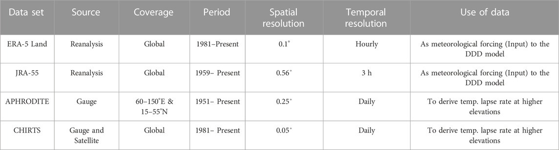
TABLE 2. Background information for selected gridded data sets.

The Shuttle Radar Topography Mission (SRTM) DEM, the Randolph Glacier Inventory (RGI V6), the Landsat-8 and Moderate Resolution Imaging Spectroradiometer (MODIS) satellite datasets are used for the current study. The SRTM DEM data were developed by the United States National Aeronautics and Space Administration (NASA) with 30 m spatial resolution. The current study used the DEM data for catchment delineation, hypsometry, river network, and hydrological model parameters (see Supplementary Table S2). The Global Land Ice Measurement from Space (GLIMS) develops the RGI dataset to monitor the glacier cover globally, with 30 m spatial resolution. The RGI data are used to derive the elevation-distributed glacier cover in the Hunza Basin (Figure 1). Landsat-8 data are developed by the Landsat Data Continuity Mission (LDCM) with 30 m spatial and 16 days temporal resolution. The Landsat-8 data are used to derive the land cover and the distances from the bogs and soil to the nearest stream of the Hunza Basin (Skaugen and Weltzien, 2016). The MODIS snow data were accessed from Muhammad et al. (2019) for the Hunza Basin. These elevation-distributed snow data were used to validate the SCA simulations by the DDD model. The DEM, RGI (V6), and Landsat-8 data are freely available and were acquired from their respective websites.

2.3 Methods

2.3.1 Model description and setup

The Distance Distribution Dynamics (DDD) model was developed by Skaugen and Onof (2014) of the Norwegian Water Resources and Energy Directorate (NVE). The model is a semi-distributed rainfall-runoff model written in the programming language Julia (Bezanson et al., 2012). The model simulates river flow, the elevation-distributed SCA, SWE, GM, actual evapotranspiration (ET) and subsurface water storage (Skaugen and Weltzien, 2016). The model is data and parameter parsimonious and only needs precipitation and temperature as input. The model has several parameters, but most are derived from digitised maps and are hence not calibrated against runoff. The model has two approaches for calculating evapotranspiration, snow and glacier melt. One with energy balance based sub-routines for snowmelt and evapotranspiration and a degree day based sub-routine for glacier melt. The second with energy balance based sub-routines for all three variables. Combined with temperature, the energy balance elements are calculated using information about geographical location, Julian day, and algorithms used in Skaugen and Saloranta (2015) and Walter et al. (2005). The model requires the basin to be divided into ten elevation zones of equal areas (a1–a10) (Supplementary Figure S1. The runoff dynamics in the Hunza Basin are described using unit hydrographs, which are determined from the GIS derived distance statistics and calibrated subsurface flow velocity (Skaugen and Mengistu, 2016). The shape parameter of gamma distribution of snow (a₀) and decorrelation length (D) are derived from spatial variability in the precipitation following Skaugen and Weltzien (2016). Supplementary Table S1 shows the model’s calibration parameters with the calibration range and values used for the current simulations. Supplementary Table S2 shows the model’s parameters derived using GIS and some parameters with fixed values. Further details on the model’s description and setup can be found in Skaugen and Onof (2014) and Nazeer et al. (2021). Note that since the application in the Gilgit Basin (Nazeer et al., 2021), the DDD model was updated adding the energy balance method for glacier melt simulation.

The DDD model requires elevation-distributed temperature and precipitation inputs. Elevation-distributed precipitation is derived from 1997 to 2010 from ERA5 and JRA-55 using climate data operators (CDO), a Linux based command line suite. About 170 ERA5 and 10 grids of JRA-55 data cover the whole Hunza Basin. To extract the precipitation data for each zone precisely and to better derive the data for the basin’s edges, both datasets were resampled to a higher resolution (1 km²), applying the nearest neighbour resampling algorithm (Nazeer et al., 2021).

2.3.2 Precipitation and temperature inputs

The gauged data and the temperature lapse rate for each zone are required to derive the elevation-distributed temperature. The gauged data was used as a reference and was assigned to the appropriate elevation zone. Naltar’s data was used for a1, Ziarat’s data for a2 and a3 and Khunjrab’s data for all remaining zones (a4–10). The average lapse rate using three stations installed at elevations 2,810, 3,669, and 4,730 masl was calculated as −6.0 C/km and applied for elevation zones a1–a6 with mean elevations from 2,321–4,745 masl. Because there are no observed temperature data for elevation zones a7-a10, the lapse rates for these elevation zones are used as a calibration parameter in the model. The range of the lapse rates for calibration is from −1 to −3 C/km, based on the analysis of the global datasets CHIRTS and APHRODITE. The calibrated lapse rate was −2.26 C/km for a7–a10.

2.3.3 Calibration and validation

The DDD model was set up for the Hunza Basin from 1997 to 2010. The period from 1997 to 2005 was used for calibration, and 2006–2010 for validation. The model was applied separately with the two methods for glacial melt: the energy balance (EB) and degree day (DD). In both cases, the model was forced with ERA5 and JRA-55 precipitation inputs separately, with the same temperature input data in all simulations. The modelling results hence include four simulations: European reanalysis 5 Land—energy balance (ERA5-EB), European reanalysis 5 Land—degree day (ERA5-DD), Japanese reanalysis 55—energy balance (JRA-EB) and Japanese reanalysis 55—degree day (JRA-DD). By applying rain and snow correction factors, the model corrects the biases in the precipitation estimates seen as over- or under-estimated runoff. All model simulations and calibration, and validation were performed on a daily time step. The model uses the first 3 months as a warm-up period, which is necessary to obtain reasonable initial soil moisture states. The Kling-Gupta efficiency (KGE) (Gupta et al. (2009) and Nash-Sutcliffe Efficiency (NSE) (Nash and Sutcliffe, 1970) were used to evaluate the model performance. Both; KGE (Eq. 1) and NSE (Eq. (2)) can take values from minus infinity to one. KGE addresses some shortcomings of the NSE (Knoben et al., 2019) and is increasingly being used for model evaluation.

$KGE=1-\sqrt{{\left(r-1\right)}^2+{\left(\frac{{\sigma }_{sim}}{{\sigma }_{obs}}-1\right)}^2+{\left(\frac{{\mu }_{sim}}{{\mu }_{obs}}-1\right)}^2}(1)$

$NSE=1-\frac{{\displaystyle \sum _{i=1}^n}{\left({Qobs}_i-{Qsim}_i\right)}^2}{{\displaystyle \sum _{i=1}^n}{\left({Qobs}_i-\overline{Qobs}\right)}^2}(2)$

Where, $r$ is the linear correlation between simulated and observed data, ${\sigma }_{sim}$ and ${\sigma }_{obs}$ are the standard deviations of simulations and observations, ${\mu }_{sim}$ and ${\mu }_{obs}$ are the means of simulations and observation, $\text{Qobs}$ _i is the observed flow and $\text{Qsimi}$ is the simulated flow, for day i$\overline{\text{Qobs}}$: mean observed flow over the number of days,

3 Results

3.1 Temperature and precipitation distribution

Supplementary Figure S2A–C shows the comparisons between gridded and gauged data for 1997–2010. The mean daily temperature derived for the current study, together with APHRODITE, CHIRTS, and gauged mean temperature, are shown in Supplementary Figure S2D. The gridded temperature estimates match well in seasonality with the gauged data, but there are also significant differences. The temperature difference decreases with elevation increase. For instance, the temperature difference between the station and APHRODITE data at the lowest station is less at the median elevation station and becomes almost zero at the highest station.

Maximum daily precipitation of 48 mm was recorded on 27 April 1997, followed by 31 mm on 25 April 2003 by ERA5. For JRA-55, maximum precipitation of 44 mm was recorded on 25 April 2003, followed by 27 mm on 27 April 1997. For mean monthly estimates (Figure 2A) by ERA5, April received maximum precipitation of 83 mm, and October received a minimum of 35 mm. For JRA-55, February received a maximum of 152 mm and September a minimum of 45 mm. These monthly estimates match reasonably well with the station data, where the Naltar recorded maximum precipitation in April, followed by February and a minimum in October, followed by November. ERA5 seasonal estimates showed that the Hunza Basin receives 27, 29, 33, and 14% precipitation during the winter, spring, monsoon and post-monsoon seasons. The JRA-55 showed 34, 35, 19, and 13% precipitation during these seasons. The seasonal estimates by ERA5 data are in good agreement with the estimates by the Naltar station. The JRA-55 performed poorly for monsoon estimates. Also, JRA-55 overestimated the precipitation with more wet days than ERA5 and gauged data. The annual estimates (Figure 2B) from 1997 to 2010 showed maximum precipitation of 947 mm and 1,322 mm in 1999 by ERA5 and JRA-55 datasets, respectively. ERA5 recorded a minimum of 594 mm in 2001, and JRA-55 recorded 822 mm in 2007. The mean annual precipitation showed 760 mm and 1,103 mm by ERA5 and JRA-55 datasets, respectively.

FIGURE 2

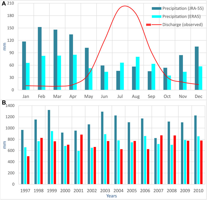
FIGURE 2. Mean (A) monthly and (B) annual precipitation from ERA5, JRA-55 data vs runoff (observed) from 1997 to 2010.

The spatial distribution of mean annual and seasonal precipitation for the Hunza Basin from 1997 to 2010 are presented in Figures 3, 4. The spatial analysis indicates that the basin receives more precipitation in the southern parts and less in the northern parts (Figure 4). The Naltar gauge is located in the basin’s south and recorded the maximum precipitation (annual mean of 718 mm) compared to the other stations. Similarly, the Khunjrab station is located on the northern edge of the basin and records the least precipitation (annual mean of 206 mm). The spatial seasonal and annual precipitation estimates by global datasets are in good agreement with the gauged data.

FIGURE 3

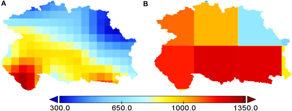
FIGURE 3. Mean annual spatial precipitation (mm) from (A) ERA5 (B) JRA-55 from 1995 to 2010.

FIGURE 4

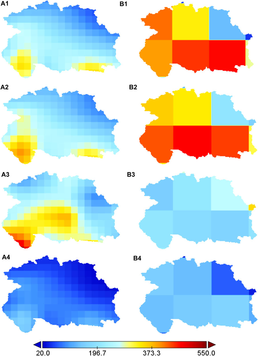
FIGURE 4. Mean seasonal spatial precipitation (mm) for (A1) ERA5 based Winter, (A2) ERA5 based Spring, (A3) ERA5 based Monsoon (A4) ERA5 based Post-monsoon, and (B1) JRA-55 based Winter, (B2) JRA-55 based Spring, (B3) JRA-55 based Monsoon (B4) JRA-55 based Post-monsoon seasons.

The altitudinal analysis of the ERA5 and JRA-55 precipitation indicated that the lower elevations received the most annual precipitation and the higher elevations received the least (Supplementary Figure S3A). The analysis further shows a negative precipitation gradient from a1 to a8 (2,321–5,159 masl), a slight negative gradient from a8 to a9 (5,160–5,407 masl), and then a strong positive from a9 to a10 (5,408–6,719 masl). These patterns are consistent in both datasets, but the seasonal analysis shows a slight negative gradient for JRA-55 (Supplementary Figure S3B) precipitation and a strong negative gradient for ERA5 (Supplementary Figure S3C) precipitation. However, monsoonal precipitation by JRA-55 indicates a slight positive gradient. At the annual/seasonal/daily scale, the gauged data show a negative precipitation gradient similar to ERA5 and JRA-55. For instance, the lower elevation gauge (Naltar, 2,810 masl) recorded its maximum annual precipitation of 832 mm in 2000, with an average of 701 mm from 1998 to 2010. The median elevation gauge (Ziarat, 3,669 masl) recorded its maximum of 578 mm in 2004, with an average of 242 mm from 1998 to 2010. The highest gauge (Khunjrab, 4,730 masl) recorded its maximum of 335 mm for 2010, with an average of 190 mm from 2003 to 2010. Similar precipitation patterns are evident for minimum precipitation records at all gauges in the Hunza Basin.

3.2 Runoff simulations

Flow simulations (Figure 5) were slightly better using ERA5-DD and achieved a KGE of 0.88 and NSE of 0.82. Simulations showed that the flow in winter is low and relatively constant at 30–35 m³/sec. The flow starts increasing in mid of April when the increase in temperature initiates the snowmelt from low-elevation areas. With further warming, snow at higher elevations and glaciers from lower elevations start contributing. With the maximum temperature in July and August, glacier melt from higher elevations starts contributing, and the flow peaks around August (1,100 m³/sec). The flow drops sharply in mid of August to less than 500 m³/sec (mean data) in mid of September. Such a sharp rise and fall in flow is also evident in the observed flow. The low flows last from December until March and are sustained by snowmelt from low elevations and groundwater discharge. The high flows last from April until November due to snow and glacier melt and peak in July/August. The 1997–2010 observed data show only 6.3% of total flow flows in the low flow period (Dec-March) and about 93.7% in the high flow period (April-Nov). These characteristic flow periods are reproduced in the simulations with slightly underestimated low flow (4%–5% of total flow) and slightly overestimated high flow (about 95% of total flow). The observed and simulated flow recessions are in good agreement for the whole period. The observed and simulated flow has several short-term peaks (mainly due to air temperature variations). The high peaks of observed flow were not simulated well by the model, but ERA5-DD is slightly better. The DDD model also simulates the actual evapotranspiration (ET) using an energy balance sub-routine based on the Priestley-Taylor equation, which is similar but simplified compared to the Penman-Monteith equation. Based on all four simulations, the minimum annual ET was from 196 to 199 mm for 2009, and the maximum was from 233 to 248 mm for 2007—the annual mean ET from 2006 to 2010 ranges from 213 to 227 mm.

FIGURE 5

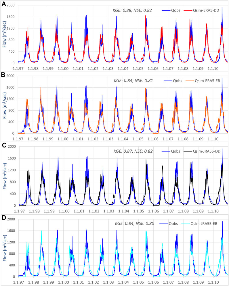
FIGURE 5. Observed runoff vs simulated (m³/sec) using (A) degree day (DD) based ERA5 (B) energy balance (EB) based ERA5 (C) degree day based JRA-55 (D) energy balance based JRA-55 simulations for calibration (1997–2005) and validation (2006–2010).

3.3 Elevation-distributed SCA and SWE

Basin-scale and elevation-distributed estimates of SCA and SWE from 2006 to 2010 for the Hunza Basin based on all four simulations are shown in Tables 3, 4. The SCA and SWE start increasing in September and peak in February. With the temperature rise in March, snow starts melting, and it keeps contributing to the flow until August. The JRA-55 based simulations showed a slightly higher SCA and SWE than ERA5. The simulated SCA is compared with the MODIS SCA derived from Muhammad et al. (2019) for 2006–2010. On the basin scale, the model simulates ERA5 and JRA-55 maximum SCA for January (99%), followed by February (95%) and a minimum in August (10%), followed by July (20%). The MODIS data have a maximum in February (85%), followed by January (82%) and a minimum in July (34%), followed by August (38%). The model has a basin scale mean annual maximum SCA of 70% in 2009 in all four simulations, and MODIS has a maximum of 66.5%, also in 2009. The minimum SCA by the model was 61% for 2006, while MODIS had 57% in 2007. The SCA simulations are consistently slightly higher than the MODIS data. For SWE, February has a maximum of 270–320 mm, and August has a minimum of 10–15 mm for all four simulations. On an annual scale (Table 3), maximum SWE was simulated in 2009 and a minimum in 2007. The JRA-EB simulation showed an annual maximum SWE (278 mm), and the ERA5-DD showed a minimum (252 mm).

TABLE 3

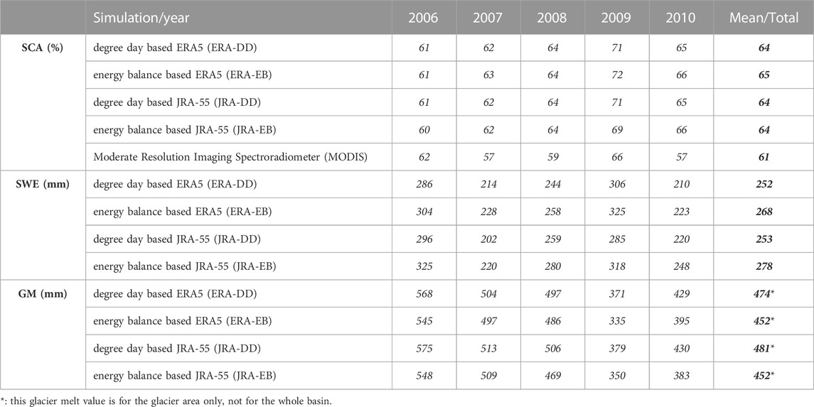
TABLE 3. Basin scale annual mean snow cover area (SCA), snow water equivalent (SWE), and glacier melt (GM) simulated by model and MODIS SCA.

TABLE 4

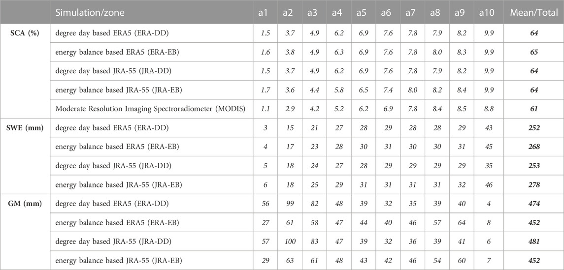
TABLE 4. Elevation-distributed annual average zonal snow cover area (SCA), snow water equivalent (SWE), and glacier melt (GM) simulated by model and MODIS SCA.

The elevation-distributed estimates (Figure 6) of SCA are also consistent and in good agreement with MODIS data. The lowest elevation was snow covered for the winter months only, while the highest elevation was covered for almost the whole year. The snow accumulation starts in September, with the higher elevation zones snow covered first. In December, almost all elevation zones are snow covered. On an annual average, the lowest zone (a1) has 15% area covered with snow by all simulations, compared to 11% in the MODIS data. The highest elevation (a10) was 100% covered with snow by the DDD model compared to 90% by the MODIS data. SCA increases linearly from a1–a10 on a monthly and annual scale, consistent with the MODIS data. Compared to the MODIS data, the simulated SCA is slightly overestimated from zone a1–a5 and in a10. The elevation-distributed simulation of SWE follows the same melt and accumulation patterns as SCA. These simulations showed the minimum annual average SWE of 3–6 mm in the lowest elevation and a maximum SWE of 35–45 mm in zone 10. High SWE at higher elevations is associated with low temperature. At higher elevations with lower temperatures, more precipitation falls as snow. The precipitation amounts can still be less at higher elevations, but since it falls as snow, there is more SWE. Similar to SCA, the mean annual SWE rises from lower to higher elevations. SWE is simulated slightly more in the energy balance approach than in the degree day approach.

FIGURE 6

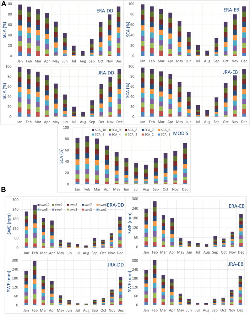
FIGURE 6. Elevation-distributed mean monthly simulated (A) snow cover area and MODIS SCA (%) (B) snow water equivalent (mm) based on all four simulations.

3.4 Elevation-distributed glacier melt

The glacier melt simulations are in good agreement with the overall seasonality and observed flow regime. According to the simulations, the glaciers contribute to the flow almost throughout the year except for the winter season (Dec–Feb). The glaciers start melting in spring, at the end of March, very insignificantly from lower elevations. When temperature increases, glaciers at higher elevations start contributing. The melt peaks in August and then declines sharply, and the contribution becomes negligible by the end of November. Based on all four simulations, the basin scale monthly average glacier melt is maximum for August with 137–148 mm. Maximum annual glacier melt to be 575 mm and 568 mm for 2006 by JRA-DD and ERA5-DD simulations. While the minimum is to be 350 mm and 335 mm for 2009 by JRA-EB and ERA5-EB simulations. The annual mean basin scale glacier melt (Table 3) is estimated as 474 and 452 mm, using ERA5-DD and ERA5-EB approaches. While it is estimated as 481 and 452 mm using JRA-DD and JRA-EB approaches.

The elevation-distributed glacier melts are presented in Figure 7. Glaciers are melting and significantly contributing to the flow from all elevations. The lowest zone (a1) starts contributing very early in spring and keeps contributing until the start of December. So, this zone contributes almost throughout the year except for the winter. After a1, a2 starts contributing at the start of April and continues until the end of November, and the glacier at higher elevations starts melting in a similar pattern. The highest zone (a10) contributes only for less than a month. These patterns of glacier melt from different elevations (Figure 7) are consistent for all simulations. However, the zonal melt contributions (Table 4) differ in the DD and EB approaches. In the degree day approach, a2 contributes the maximum (21%), followed by a3 (17%) of total glacier melt. While for the energy balance approach, a9 contributes the maximum (14%), followed by a3 (13%). For the minimum contributions, both approaches identified a10 (1%–2%) followed by a6 (7%–9%) in degree day and a1 (6%) in energy balance. The lower half of the basin (a1–a5), with 32% of the total glacier cover, is more active and contributes more than 50% of the total glacier runoff. More contributions from lower zones are consistent for all four simulations. However, the energy balance based sub-routine shows a slightly higher melt contribution from higher elevations.

FIGURE 7

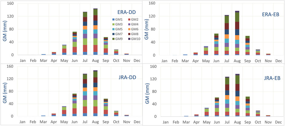
FIGURE 7. Elevation-distributed mean monthly simulated glacier melt (mm) based on all four simulations.

3.5 Water balance

In a glaciated catchment, the water balance (WB) can be represented as;

$P\pm GM=Q+ET\pm \Delta S(3)$

Where $P$ is precipitation, $GM$ is the glacier melt contribution, $Q$ is the runoff from the catchment (both surface and subsurface), $ET$ is the actual evapotranspiration and $\Delta S$ is the change in storages.

Table 5 shows an analysis of the inflow/outflow composition and water balance (Eq. (3)) from all four simulations on the annual scale. Figure 8 shows the same on the mean monthly scale from 2006 to 2010. The inflow components are precipitation (rain and snow) and glacier melt. The outflow includes simulated flow and actual evapotranspiration. On the annual scale, the ΔS is assumed negligible in the water balance equation. The winter months have the minimum outflow because most precipitation falls as snow. This stored snow starts contributing to the runoff in spring, and the outflow rises significantly. With further temperature and energy rise, glacier melt also contributes significantly and flow peaks in July/August. ET also peaks in July and August. The outflow starts declining significantly in September and is at a minimum in December/January. The runoff contributions in low and high flow periods are consistent in all four simulations. The mean annual contribution of snowmelt to the runoff is estimated to be 30%–34%, and the contribution from rain precipitation is 21%–23.5%. On average, the JRA-EB and ERA5-DD simulations showed the maximum (33.8%), and minimum (30.7%) snowmelt contribution to the runoff, respectively. For the rainfall contribution, the ERA5-EB simulation showed the maximum (23.5%), and the JRA-EB simulation showed the minimum. Results further showed that the Hunza River receives 44%–48% of its total flow from glacier melt based on all four simulations. The maximum (47.6%) glacier melt contribution was simulated by JRA-DD, and the minimum (44.1%) by ERA5-EB. For the outflows (Q + ET), results showed a mean annual runoff 78%–79% and actual evapotranspiration 21%–22%.

TABLE 5

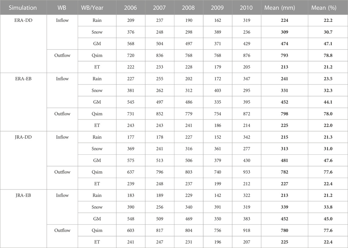
TABLE 5. Annual water balance of the Hunza Basin based on all four simulations.

FIGURE 8

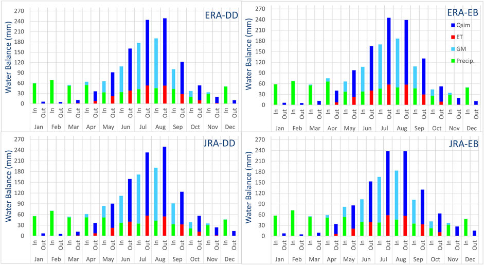
FIGURE 8. Mean Monthly water balance (mm) of the Hunza Basin based on all four simulations.

4 Discussion

The temperature plays a critical role in the snow- and glacier-dominated basins like the Hunza. The very few and non-uniformly distributed temperature measurement stations proved a significant limitation for deriving accurate elevation-distributed temperature. However, a realistic, elevation-distributed temperature is essential for simulating hydrologic processes. Fixed lapse rate values ranging from −2.3 to −9.2 ^°C/km were applied in the Hunza Basin in previous studies (Tahir et al., 2011; Immerzeel et al., 2012; Ragettli and Pellicciotti, 2012; Shrestha et al., 2015; Garee et al., 2017). However, the lapse rate derived from the available temperature measurements does not support using a single (constant) lapse rate value for the entire elevation range, and there is no in situ measured temperature data to assess the lapse rate for elevations higher than 4,730 masl. In this study, two lapse rates were used. One for a1-a6 based on observed data and one for a7-a10, which is calibrated using lapse rate range from global datasets. The modelling approach (the DDD model) with elevation-distributed temperature and precipitation inputs gave reasonable results.

Precipitation is a major source of uncertainty in the Hunza basin. Mean annual areal precipitation estimated in the previous studies varies between about 700 and 1,000 mm, e.g., 731 mm for 2001–2003 (Shrestha and Nepal, 2019), 828 mm for 2001–2003 (Immerzeel et al., 2012), 733 mm for 1998–2012 (Dahri et al., 2021), and about 1,000 mm for 1971–2000 (Lutz et al., 2014). However, the basin-scale precipitation estimates suffer from inadequate and unevenly distributed in situ measurements. The use of the gridded data allowed us to show the variation of precipitation with elevation, which would not be possible using in situ observations from only three available stations. The temporal precipitation distribution indicates that the Hunza Basin receives significant precipitation as snow during the winter and spring seasons. The spatial estimates indicate a clear northeast to southwest increase in precipitation with a maximum on the southern edge of the basin. The Batura glacier acts as a precipitation dividing wall between the south and north of the Hunza Basin (Winiger et al., 2005). This barrier effect intensifies the southwest-northeast decrease of precipitation; consequently, the southwest part of the basin receives more precipitation.

The ERA5 and JRA-55 data used in the current study showed an overall negative precipitation gradient for the Hunza Basin. These patterns are consistent in both datasets at daily, monthly and seasonal scales. This find is consistent with previous reports. Hewitt (2011) concluded that the maximum precipitation in the Hunza Basin occurs between 5,000 and 6,000 masl. They associated glacier expansion in the basin with higher winter precipitation at higher elevations. Pang et al. (2014) suggest a decreasing precipitation gradient at elevations above 2,400 masl in the central Himalayas. Dahri et al. (2016) also concluded that the precipitation increases up to a certain elevation (around 2,500 masl) and decreases after that, so establishing any linear equation between precipitation and elevation in the HKH region is unsuitable. Immerzeel et al. (2012), in their study in the Nepalese Himalayas, concluded that it is difficult to establish a constant precipitation gradient due to the influence of local orographic effects and complex weather system.

The comparison of the observed and simulated runoff hydrographs and model performance indicators showed that the DDD model reproduces the inter- and intra-annual variability reasonably well. The simulation results using ERA5 and JRA-55 as precipitation input data suggest that these products are suitable alternatives to observations for such a high-altitude and data-scarce basin. The ERA5 simulation showed slightly better NSE and KGE, probably due to its higher spatial resolution. The flow in the Hunza Basin mainly comes from snow and glacier melt, as the basin lies in a westerlies-influenced region. The simulation results match the overall seasonality and observed flow of the Hunza River. The model performance indicators (NSE and KGE) achieved in all four simulations are reasonable and consistent. The flow recession matches very well in all simulations. The peak flow timing in the observed and simulated hydrographs is slightly different. Primary reasons for this are possibly the errors in the spatial distribution of snow and uncertainties in the input data (precipitation and temperature). However, uncertainties in the model parameters and structure may have contributed to this. The gridded data sets (ERA and JRA) also have temporal and spatial resolution limitations and limited ability to reproduce extremes (Kidd et al., 2013). In addition, these datasets (especially JRA-55) perform inadequately in capturing the monsoon rainfall. Consequently, the sharp flow peaks by the monsoon in summer are not reproduced well in the current simulations.

The observed and simulated hydrographs are shown on a daily time step. In general, the low flows are underestimated, but the results are mixed in the case of high/peak flows (some are overestimated, some are underestimated). Such a model performance (reasonably good for long-term overall performance indicated by reasonably high NSE values, but under/overestimation of low/high flows) is not unusual for a basin with very high intra-annual variation of daily discharge. The under/over estimations of low/high flows are usually a result of a several things, primarily the course resolution or lack of data and simplification or limitation of some aspects of the model. In this basin, the low flow occurs during the winter months, when the precipitation falls as snow and due to low temperature snow/glacier melt is almost nonexistence. Thus, the low flows in the winter are from the groundwater. The DDD model is aimed at snow/glacier fed runoff, and its groundwater simulation is not particularly strong. The high flows in this basin are driven by the snow/glacier melt and monsoon rainfall. In the case of high flows, the under/over estimations are more likely due to the lack of in suti measurement data (particularly at high elevation areas) than the model equations or parameters. However, the model parameterization also plays a role, because for the long-term continuous simulation, the parameters are not aimed only at getting the peak flows right but the overall performance (indicated by the NSE).

Tahir et al. (2011) also underestimated the peak flows for the Hunza Basin, and they associated this with their precipitation input. Such discrepancies in observed and simulated flow were also observed by Shrestha et al. (2015) for the Hunza Basin from 2003 to 2004, and they associated it with uncertainty in the input data. Dahri et al. (2021) also concluded that accurate assessments of hydrologic processes in the high-altitude Indus Basin are challenging because of the unavailability of reliable input data. Reggiani and Rientjes (2015) estimated the mean evapotranspiration as 200 ± 100 mm/year for the UIB from 1961 to 2009. Bhutiyani (1999) estimated this as 222 mm/year for the Siachen glacier (Nubra valley of eastern Karakoram) from 1986 to 1991. Hence, the current estimates of mean annual ET (213–227 mm) are similar to previous findings.

Simulating a realistic snow cover and snow water equivalent is essential for understanding the hydrological processes in the Hunza basin. Hasson et al. (2014) presented almost similar estimates to this study of SCA with 83% ± 4% during the winter/spring season and 17% ± 6% during the summer season from 2001 to 2012 for the Hunza Basin. Similar estimates were presented by Tahir et al. (2011), with SCA varying between 30% in summer and 80% in winter for the Hunza Basin from 2000 to 2004. Shrestha and Nepal (2019) presented SCA estimates between 30% in summer and 87% in winter for the Hunza Basin from 2000 to 2010. The DDD model slightly overestimates the SCA compared with the MODIS data for the winter season. Although precipitation by global datasets were corrected by the model using correction factors, precipitation still may have uncertainties. This overestimation may also be associated with limitations in the model’s structure, where the model estimates the entire elevation zone as snow covered in case of snow event. Moreover, only 10% of the Hunza’s area is located under an elevation of 3,217 m, so due to low temperature in winter, the whole basin would be snow covered if it rains in winter. As mentioned before, this basin is located in westerlies influenced region where most of the precipitation falls in winter as snow. For summer, the simulations show that the basin has about 10% SCA, while MODIS has about 40%. This discrepancy is due to the presence of permanent glaciers (RGI 6.0) in the basin that have been classified as snow cover in the MODIS data. The DDD model keeps track of SCA and glaciers separately. Also, the MODIS snow data has coarse temporal (8-day) resolution, but the snow cover area may change day by day when melting starts.

The significant glacier melt contribution from the least glaciated lowest zones (a1, a2) and the least from the highly glaciated zone (a10) show how temperature impacts more significantly than the glacier extent. There are some differences in the glacier melt contributions from different elevation zones in the two sub-routines (Table 4). The degree day sub-routine melts more from lower elevations with a maximum from zone a2. The energy balance approach produces slightly more than the DD sub-routine from higher elevations with maximum melts from zones a2 and a9. The degree day based sub-routine is based on a calibrated degree-day factor and is totally dominated by temperature. The energy balance subroutine does not involve any calibrated parameter and simulates the glacier melt using radiation and temperature. In both sub-routines, the highest zones (a10) with maximum glacier coverage melts least because of the very low temperature at such higher elevations (5,550–7,889 masl).

Snowmelt is significant from spring to late summer (mid-April to mid-October), and some snowmelt continues throughout the year. Simulations showed a time overlap in snow and glacier melts (Supplementary Figure S4). That means that the glacier melt from lower elevations starts contributing when there is still snow left at higher elevations of the basin. The glacier cover of the Hunza Basin starts at 2,300 masl (Hewitt, 2014), so temperature rise in spring/early summer at these elevations can melt glaciers. Also, if the precipitation falls as snow in the glacier melt season on some elevation zones, the snow may quickly melt while the glacier is also melting in snow free zones. Similar overlap patterns are evident in the accumulation season. The snow accumulates, and the glacier melt contribution decreases with temperature decline, but glaciers from lower elevations are still melting. So separating these snow and glacier melt regimes based on the month, as done by Mukhopadhyay and Khan (Mukhopadhyay and Khan, 2014, Mukhopadhyay and Khan, 2015), does not apply in the current study.

Mukhopadhyay and Khan (2015) presented flow composition based on generic flow regimes analysis and hydrograph separation using historical monthly flow data for the Hunza River for two periods. From 1966 to 1979, they estimated the base flow (flow due to precipitation as rain plus remnant melt) contribution as 22.5%, snowmelt as 31.85%, and glacier melt as 45.65%. From 1980 to 2010, they estimated base flow as 27.98%, snowmelt as 32.52%, and glacier melt as 39.49%. Shrestha and Nepal (2019) presented the annual mean flow composition for the Hunza Basin from 2001 to 2003 as snowmelt with 45%, glacier melt with 47%, and rain with 9%. Shrestha et al. (2015) presented these contributions as 50% by snowmelt, 33% by glacier melt, and 17% by precipitation as rain for the Hunza Basin. The flow composition from the current study substantiates the previous findings, where glacier melt contributed 44%–48%, snowmelt 30%–34%, and rain as precipitation 21%–23.5% to the runoff. Moreover, the current study also quantified the snow and glacier melts from different elevation zones.

4.1 Limitations of the study

The quality and reliability of input data (mainly temperature and precipitation) are crucial in hydrological modelling. Also, the accuracy of the modelling results largely depends on the modelling framework. As typical of data-scarce basin, this study also has several limitations associated with input data and model structure. In the HKH region, it is very challenging to get consistent long-term data which become one of the main limitations. Temperature inputs are very critical in a melt dominant catchment like the Hunza. However, the temperature for higher elevations is based on coarse assumptions such as the linear change in temperature with elevation. The zonal precipitation was derived using global products with a low spatial resolution (particularly the JRA-55), given the high spatial variability in the basin and limited ability to capture extremes. Hence, the precipitation estimates may still have biases and including more observed data can bring us closer to the truth. The flow data used for calibration/validation are assumed to be sufficiently accurate compared to climatic data, considering the measurement techniques and data quality. However, the flow data may still have uncertainties due to measurement errors. Nespak-Aht-Deltares (2015) evaluated river/canal flow measurement protocols of the Indus River system and observed overall 3%–8% uncertainties at five canal headworks.

The DDD hydrological model used in the current study is validated and applied with four different sets of inputs/sub-routines, and no significant drawbacks are found in the modelling structure. The simplified equations in the energy balance sub-routines for snowmelt, glacier melt and evapotranspiration have shown promising results. Yet, the model has a coarse representation of topography, neglects wind speed and the model seem to overestimate the SCA. The calibrated parameters in the model are not validated against observations from the study area. In the current DDD model setup, debris-covered and debris-free glaciers are not distinguished. The melt rate for debris-covered glaciers usually differs from debris-free glaciers, which is of one the sources of uncertainty in glacier melt simulation.

5 Conclusion

The modelling framework included four simulations based on two glacier melt approaches and two precipitation inputs. The data parsimonious precipitation-runoff model, Distance Distribution Dynamics (DDD), was applied to the Hunza Basin. The elevation-distributed precipitation and melt simulations and the overall water balance of the basin were analysed. The key findings are as follows:

• Elevation-distributed precipitation estimates are presented based on recently developed and better performing gridded products. Most of the precipitation (57%–69%) in the Hunza Basin falls in the winter and spring season (Dec-April/May). The analysis showed more precipitation at lower elevations than at higher. A simple linear elevation-dependent precipitation gradient is unsuitable for high-altitude basins like the Hunza, with a complex topography and multiple weather systems.

• The modelling results showed that the DDD model could reproduce the runoff satisfactorily, with KGE ranging from 0.84 to 0.88 and NSE ranging from 0.80 to 0.82. The DDD model is found to be reliable for such high altitude, snow- and glacier-dominated and data-scarce basins.

• The river flow in the study area depends more on glacier melt (45%–48%), followed by snowmelt (30%–34%) and rainfall (21%–23%). The annual mean actual evapotranspiration is 21%–22% of the total outflow. The study presents more realistic elevation-distributed GM simulations where the lower half of the basin, with 32% of the total glacier cover, is more active, with more than 50% of the total glacier melt. The elevation-distributed simulated SCA was validated with an independent SCA from MODIS, and the results are in good agreement.

• Elevation-distributed glacier melt analysis indicates the glacier has a significant impact on the flow regime of the area. Although the degree day sub-routine based simulation slightly improves efficiency, the energy balance sub-routine seems more realistic; because the energy balance subroutine does not involve any calibrated parameter and simulates the glacier melt using radiation and temperature.

• The snow and glacier melts appear simultaneously from April to October. As the glaciers are distributed throughout the basin, the temperature increases in early summer, melting glaciers at lower elevations and snow at higher elevations. Also, if the precipitation falls as snow during the glacier melt season at higher altitudes, it may start contributing to the river flow while glacier melt continues in the lower elevation.

• Based on the findings from a comparatively new modelling framework and gridded precipitation data, an improved understanding of the hydrology of the Hunza Basin is presented. Our results showed that the glaciers at lower elevations with less coverage contribute more to the river runoff than those at higher elevations. Moreover, the validation of the simulated elevation-distributed snow cover area using the independent satellite data supported the accuracy of the modelling approach. The simulation showed that the DDD model reproduces the hydrological processes satisfactorily for such a data-scarce basin. The findings improve understanding by providing helpful information about the water balance and hydro-climatic regimes. Lutz et al., 2016.

Data availability statement

The original contributions presented in the study are included in the article/Supplementary Material, further inquiries can be directed to the corresponding author.

Author contributions

Conception and design of study: AN, SM, and MC. Acquisition of data: AN, SM, and TS. Analysis and/or interpretation of data: AN, SM, TS, and MM. Drafting the manuscript: AN, SM, TS, and MM. Revising the manuscript critically for important intellectual content: AN, SM, TS, and MM. Approval of the version of the manuscript to be published: AN, SM, TS, and MM. All authors contributed to the article and approved the submitted version.

Funding

AN is financially sponsored through a development project of the Higher Education Commission (HEC) Pakistan titled “Strengthening of Bahauddin Zakariya University (BZU) Multan, Pakistan”.

Acknowledgments

The authors extend their thanks to the Water and Power Development Authority (WAPDA) and the Pakistan Meteorological Department (PMD) for sharing the hydrological and meteorological data.

Conflict of interest

The authors declare that the research was conducted in the absence of any commercial or financial relationships that could be construed as a potential conflict of interest.

Publisher’s note

All claims expressed in this article are solely those of the authors and do not necessarily represent those of their affiliated organizations, or those of the publisher, the editors and the reviewers. Any product that may be evaluated in this article, or claim that may be made by its manufacturer, is not guaranteed or endorsed by the publisher.

Supplementary material

The Supplementary Material for this article can be found online at: https://www.frontiersin.org/articles/10.3389/feart.2023.1215878/full#supplementary-material

References

Archer, D. R., and Fowler, H. J. (2004). Spatial and temporal variations in precipitation in the Upper Indus Basin, global teleconnections and hydrological implications. Hydrology Earth Syst. Sci. 8, 47–61. doi:10.5194/hess-8-47-2004

CrossRef Full Text | Google Scholar

Arendt, A., (2017). Randolph Glacier inventory–A dataset of global glacier outlines: Version 6.0: Technical report, global land Ice measurements from Space. Plymouth USA. RGI Consortium.

Google Scholar

Barnett, T. P., Adam, J. C., and Lettenmaier, D. P. (2005). Potential impacts of a warming climate on water availability in snow-dominated regions. Nature 438, 303–309. doi:10.1038/nature04141

PubMed Abstract | CrossRef Full Text | Google Scholar

Bhutiyani, M. (1999). Mass-balance studies on Siachen glacier in the nubra valley, Karakoram Himalaya, India. J. Glaciol. 45, 112–118. doi:10.3189/s0022143000003099

CrossRef Full Text | Google Scholar

Bolch, T. (2017). Asian glaciers are a reliable water source. Nature 545, 161–162. doi:10.1038/545161a

PubMed Abstract | CrossRef Full Text | Google Scholar

Bookhagen, B., and Burbank, D. W. (2006). Topography, relief, and TRMM-derived rainfall variations along the Himalaya. Geophys. Res. Lett. 33, L08405. doi:10.1029/2006gl026037

CrossRef Full Text | Google Scholar

Bookhagen, B., and Burbank, D. W. (2010). Toward a complete himalayan hydrological budget: spatiotemporal distribution of snowmelt and rainfall and their impact on river discharge. J. Geophys. Res. Earth Surf. 115, F03019. doi:10.1029/2009jf001426

CrossRef Full Text | Google Scholar

Dahri, Z. H., Ludwig, F., Moors, E., Ahmad, B., Khan, A., and Kabat, P. (2016). An appraisal of precipitation distribution in the high-altitude catchments of the Indus basin. Sci. Total Environ. 548, 289–306. doi:10.1016/j.scitotenv.2016.01.001

PubMed Abstract | CrossRef Full Text | Google Scholar

Dahri, Z. H., Ludwig, F., Moors, E., Ahmad, S., Ahmad, B., Ahmad, S., et al. (2021). Climate change and hydrological regime of the high-altitude Indus basin under extreme climate scenarios. Sci. Total Environ. 768, 144467. doi:10.1016/j.scitotenv.2020.144467

PubMed Abstract | CrossRef Full Text | Google Scholar

Funk, C., Peterson, P., Peterson, S., Shukla, S., Davenport, F., Michaelsen, J., et al. (2019). A high-resolution 1983–2016 T max climate data record based on infrared temperatures and stations by the Climate Hazard Center. J. Clim. 32, 5639–5658. doi:10.1175/jcli-d-18-0698.1

CrossRef Full Text | Google Scholar

Garee, K., Chen, X., Bao, A., Wang, Y., and Meng, F. (2017). Hydrological modeling of the upper Indus Basin: A case study from a high-altitude glacierized catchment Hunza. Water 9, 17. doi:10.3390/w9010017

CrossRef Full Text | Google Scholar

Gupta, H. V., Kling, H., Yilmaz, K. K., and Martinez, G. F. (2009). Decomposition of the mean squared error and nse performance criteria: implications for improving hydrological modelling. J. hydrology 377, 80–91. doi:10.1016/j.jhydrol.2009.08.003

CrossRef Full Text | Google Scholar

Hall, D. K., and Riggs, G. A. (2007). Accuracy assessment of the MODIS snow products. Hydrological Process. An Int. J. 21, 1534–1547. doi:10.1002/hyp.6715

CrossRef Full Text | Google Scholar

Hasson, S., Lucarini, V., Khan, M. R., Petitta, M., Bolch, T., and Gioli, G. (2014). Early 21st century snow cover state over the Western river basins of the Indus River system. Hydrology Earth Syst. Sci. 18, 4077–4100. doi:10.5194/hess-18-4077-2014

CrossRef Full Text | Google Scholar

Hasson, S. u. (2016). Future water availability from Hindukush-Karakoram-Himalaya Upper Indus Basin under conflicting climate change scenarios. Climate 4 (40), 40. doi:10.3390/cli4030040

CrossRef Full Text | Google Scholar

Hewitt, K. (2011). Glacier change, concentration, and elevation effects in the Karakoram Himalaya, upper Indus Basin. Mt. Res. Dev. 31, 188–200. doi:10.1659/mrd-journal-d-11-00020.1

CrossRef Full Text | Google Scholar

Hewitt, K. (2014). Glaciers of the Karakoram Himalaya. Berlin, Germany Springer.

Google Scholar

Immerzeel, W., Wanders, N., Lutz, A. F., Shea, J. M., and Bierkens, M. F. P. (2015). Reconciling high-altitude precipitation in the upper Indus basin with glacier mass balances and runoff. Hydrology Earth Syst. Sci. 19, 4673–4687. doi:10.5194/hess-19-4673-2015

CrossRef Full Text | Google Scholar

Immerzeel, W. W., Pellicciotti, F., and Shrestha, A. B. (2012). Glaciers as a proxy to quantify the spatial distribution of precipitation in the Hunza basin. Mt. Res. Dev. 32, 30–38. doi:10.1659/mrd-journal-d-11-00097.1

CrossRef Full Text | Google Scholar

Kayastha, R. B., and Kayastha, R. (2020). “Glacio-hydrological degree-day model (GDM) useful for the Himalayan River basins,” in Himalayan weather and climate and their impact on the environment. Editors A. Dimri, B. Bookhagen, M. Stoffel, and T. Yasunari Berlin, Germany (Cham: Springer), 379–398.

CrossRef Full Text | Google Scholar

Kidd, C., Dawkins, E., and Huffman, G. (2013). Comparison of precipitation derived from the ECMWF operational forecast model and satellite precipitation datasets. J. Hydrometeorol. 14, 1463–1482. doi:10.1175/jhm-d-12-0182.1

CrossRef Full Text | Google Scholar

Knoben, W. J., Freer, J. E., and Woods, R. A. (2019). Inherent benchmark or not? Comparing nash–sutcliffe and kling–gupta efficiency scores. Hydrology Earth Syst. Sci. 23, 4323–4331. doi:10.5194/hess-23-4323-2019

CrossRef Full Text | Google Scholar

Kobayashi, S., Ota, Y., Harada, Y., Ebita, A., Moriya, M., Onoda, H., et al. (2015). The jra-55 reanalysis: general specifications and basic characteristics. J. Meteorological Soc. Jpn. Ser. II 93, 5–48. doi:10.2151/jmsj.2015-001

CrossRef Full Text | Google Scholar

Lutz, A. F., Immerzeel, W. W., Kraaijenbrink, P. D. A., Shrestha, A. B., and Bierkens, M. F. P. (2016). Climate change impacts on the upper indus hydrology: sources, shifts and extremes. PloS one 11, e0165630. doi:10.1371/journal.pone.0165630

PubMed Abstract | CrossRef Full Text | Google Scholar

Lutz, A., Immerzeel, W. W., Shrestha, A. B., and Bierkens, M. F. P. (2014). Consistent increase in High Asia's runoff due to increasing glacier melt and precipitation. Nat. Clim. Change 4, 587–592. doi:10.1038/nclimate2237

CrossRef Full Text | Google Scholar

Martinec, J. (1975). Snowmelt-runoff model for stream flow forecasts. Hydrology Res. 6 (3), 145–154. doi:10.2166/nh.1975.0010

CrossRef Full Text | Google Scholar

Maskey, S. (2022). Catchment hydrological modelling: The science and art. Amsterdam, Netherlands Elsevier. doi:10.1016/C2018-0-03853-0

CrossRef Full Text | Google Scholar

Muhammad, S., Tian, L., and Khan, A. (2019). Early twenty-first century glacier mass losses in the Indus Basin constrained by density assumptions. J. hydrology 574, 467–475. doi:10.1016/j.jhydrol.2019.04.057

CrossRef Full Text | Google Scholar

Mukhopadhyay, B., and Khan, A. (2014). A quantitative assessment of the genetic sources of the hydrologic flow regimes in Upper Indus Basin and its significance in a changing climate. J. hydrology 509, 549–572. doi:10.1016/j.jhydrol.2013.11.059

CrossRef Full Text | Google Scholar

Mukhopadhyay, B., and Khan, A. (2015). A reevaluation of the snowmelt and glacial melt in river flows within Upper Indus Basin and its significance in a changing climate. J. hydrology 527, 119–132. doi:10.1016/j.jhydrol.2015.04.045

CrossRef Full Text | Google Scholar

Nash, J. E., and Sutcliffe, J. V. (1970). River flow forecasting through conceptual models part I—a discussion of principles. J. hydrology 10, 282–290. doi:10.1016/0022-1694(70)90255-6

CrossRef Full Text | Google Scholar

Nazeer, A., Maskey, S., Skaugen, T., and McClain, M. E. (2021). Simulating the hydrological regime of the snow fed and glaciarised gilgit basin in the upper indus using global precipitation products and a data parsimonious precipitation-runoff model. Science of the Total Environment, 802 149872. doi:10.1016/j.scitotenv.2021.149872

PubMed Abstract | CrossRef Full Text | Google Scholar

Nespak-Aht-Deltares, (2015). Improvement of water Resources management of Indus Basin to enhance the capacity of Indus River system authority, Islamabad, Pakistan, Indus River System Authority.

Google Scholar

Pang, H., Hou, S., Kaspari, S., and Mayewski, P. A. (2014). Influence of regional precipitation patterns on stable isotopes in ice cores from the central Himalayas. Cryosphere 8, 289–301. doi:10.5194/tc-8-289-2014

CrossRef Full Text | Google Scholar

Qureshi, M. A., Yi, C., Xu, X., and Li, Y. (2017). Glacier status during the period 1973–2014 in the Hunza Basin, western Karakoram. Quat. Int. 444, 125–136. doi:10.1016/j.quaint.2016.08.029

CrossRef Full Text | Google Scholar

Ragettli, S., and Pellicciotti, F. (2012). Calibration of a physically based, spatially distributed hydrological model in a glacierized basin: on the use of knowledge from glaciometeorological processes to constrain model parameters. Water Resour. Res. 48. doi:10.1029/2011wr010559

CrossRef Full Text | Google Scholar

Raza, S. A., Ali, Y., and Mehboob, F. (2012). Role of agriculture in economic growth of Pakistan, International Research Journal of Finance and Economics, 83Available at: https://mpra.ub.uni-muenchen.de/32273/

Google Scholar

Reggiani, P., and Rientjes, T. (2015). A reflection on the long-term water balance of the Upper Indus Basin. Hydrology Res. 46, 446–462. doi:10.2166/nh.2014.060

CrossRef Full Text | Google Scholar

Shrestha, M., Koike, T., Hirabayashi, Y., Xue, Y., Wang, L., Rasul, G., et al. (2015). Integrated simulation of snow and glacier melt in water and energy balance-based, distributed hydrological modeling framework at Hunza River Basin of Pakistan Karakoram region. J. Geophys. Res. Atmos. 120, 4889–4919. doi:10.1002/2014jd022666

CrossRef Full Text | Google Scholar

Shrestha, S., and Nepal, S. (2019). Water balance assessment under different glacier coverage scenarios in the Hunza Basin. Water 11, 1124. doi:10.3390/w11061124

CrossRef Full Text | Google Scholar

Skaugen, T., and Mengistu, Z. (2016). Estimating catchment-scale groundwater dynamics from recession analysis–enhanced constraining of hydrological models. Hydrology Earth Syst. Sci. 20, 4963–4981. doi:10.5194/hess-20-4963-2016

CrossRef Full Text | Google Scholar

Skaugen, T., and Onof, C. (2014). A rainfall-runoff model parameterized from GIS and runoff data. Hydrol. Process. 28, 4529–4542. doi:10.1002/hyp.9968

CrossRef Full Text | Google Scholar

Skaugen, T., and Saloranta, T. (2015). Simplified energybalance snowmelt modelling. Oslo, Norway, Norwegian Water Resources and Energy Directorate Rep. 31.

Google Scholar

Skaugen, T., and Weltzien, I. H. (2016). A model for the spatial distribution of snow water equivalent parameterized from the spatial variability of precipitation. Cryosphere 10, 1947–1963. doi:10.5194/tc-10-1947-2016

CrossRef Full Text | Google Scholar

Tahir, A. A., Chevallier, P., Arnaud, Y., Neppel, L., and Ahmad, B. (2011). Modeling snowmelt-runoff under climate scenarios in the Hunza River basin, Karakoram range, northern Pakistan. J. hydrology 409, 104–117. doi:10.1016/j.jhydrol.2011.08.035

CrossRef Full Text | Google Scholar

Terink, W., Lutz, A. F., Simons, G. W. H., Immerzeel, W. W., and Droogers, P. (2009–2034). Sphy v2.0: spatial processes in hydrology. Geosci. Model Dev. 8, 2009–2034. doi:10.5194/gmd-8-2009-2015

PubMed Abstract | CrossRef Full Text | Google Scholar

Walter, M. T., Brooks, E. S., McCool, D. K., King, L. G., Molnau, M., and Boll, J. (2005). Process-based snowmelt modeling: does it require more input data than temperature-index modeling? J. hydrology 300, 65–75. doi:10.1016/j.jhydrol.2004.05.002

CrossRef Full Text | Google Scholar

Winiger, M., Gumpert, M., and Yamout, H. (2005). Karakorum–hindukush–western himalaya: assessing high-altitude water resources. Hydrological Process. An Int. J. 19, 2329–2338. doi:10.1002/hyp.5887

CrossRef Full Text | Google Scholar

Yatagai, A., Kamiguchi, K., Arakawa, O., Hamada, A., Yasutomi, N., and Kitoh, A. (2012). Aphrodite: constructing a long-term daily gridded precipitation dataset for asia based on a dense network of rain gauges. Bull. Am. Meteorological Soc. 93, 1401–1415. doi:10.1175/bams-d-11-00122.1

CrossRef Full Text | Google Scholar

Young, G. J. (1985). Snow and glacier hydrology. Wallingford, Oxfordshire, UK, International Association of Hydrological Sciences.

Google Scholar