Decadal modulation of ENSO and IOD impacts on the Indian Ocean upwelling

The decadal modulations are observed in impacts of El Niño and Southern Ocean (ENSO) and Indian Ocean Dipole (IOD) on the tropical Indian Ocean upwelling. Here, we explore important contributors to the decadal modulations by combining the observational data since 1958 and statistical model simulations. A Bayesian Dynamic Linear Model (BDLM), which represents the temporal modulations of the IOD and ENSO impacts, reproduces the timeseries of the eastern and western Indian Ocean (EIO and WIO) upwellings more realistically than a conventional Static Linear regression Model does. The time-varying regression coefficients in BDLM indicate that the observed shift of the IOD impact on the EIO upwelling around 1980 is mainly due to the changes of alongshore wind stress forcing and the sensitivity of the upper ocean temperature in the EIO through the surface warming tendency and the enhanced ocean stratification. In contrast, the impacts of ENSO and IOD on the WIO are modulated in relation to the decadal variability of the tropical Pacific Ocean. When the eastern tropical Pacific Ocean is observed warmer on decadal timescales, the accompanying changes of the dominant ENSO flavors contribute to modulating the strengths of the atmospheric convective activity over the Indian-Pacific warm pool and the easterly wind variations in the equatorial Indian Ocean.

Highlights

• A Bayesian Dynamic Linear Model (BDLM), which represents the temporal modulations of the IOD and ENSO impacts, reproduces the timeseries of the eastern and western Indian Ocean upwellings better than a conventional Static Linear regression Model does.

• The BDLM results indicate that the IOD impact on the EIO upwelling is significantly modulated primarily due to the stronger ocean stratification in addition to the stronger surface wind forcing after 1980s than before.

• The ENSO impact on the WIO upwelling is also decadally modulated mainly due to differences in the dominant ENSO patterns linked to PDO phase.

1 Introduction

In the Indian Ocean, intense seasonally reversing monsoon wind forcing prevails, more specifically, southeasterly wind dominates in the southern Indian Ocean through the year, and north easterly wind blows along Somalia, Oman in January and reverse in July (see Figure 2 in Han et al., 2017). In response to the seasonally changed monsoon forcing, the alongshore current (Somalia current) also reverse during January and July. In both the eastern Indian Ocean (EIO) and the western Indian Ocean (WIO), seasonal and annual mean upwelling occurs (see Figure 1; Zhang and Han, 2020). In the western basin around 12^oS-2^oS, open-ocean upwelling exists (McCreary et al., 1993; Murtugudde et al., 1999), which is also referred to as the Seychelles–Chagos thermocline ridge (SCTR; Hermes and Reason, 2008; Yokoi et al., 2008; 2009) and in contract, seasonally changed upwelling occurs along the coastal area of EIO only during boreal summer (Figure 1C; Susanto et al., 2001; Schott et al., 2009).

FIGURE 1

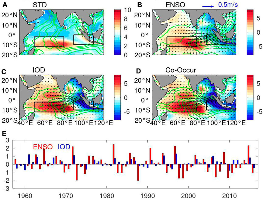
FIGURE 1. (A) Standard deviation of SSHA (color shading, unit: cm) and precipitation (contour, unit: mm/day) during 1958–2016. Composite maps of SSHA, precipitation anomaly and zonal and meridional wind anomalies at 1000 hPa (vectors, unit:m/s) of (B) El Nino events, (C) positive IOD events and (D) co-occur events from 1958 to 2016. The SSHA is based on ORAS4 data, the wind is from NCEP data, and the precipitation data is from NOAA. The black boxes indicate the eastern Indian Ocean (EIO) and western Indian Ocean (WIO) mean upwelling zones. The El Nino and positive IOD events are defined from NOAA website. (E) Time series of seasonal means of the ENSO index (red bars; November-January) and IOD index (blue bars; September-November).

One of the key processes of the upwelling formation is contribution of oceanic Rossby waves, possibly together with local Ekman Pumping (e.g., Tozuka et al., 2010; Trenary and Han, 2012). Previous works have also suggested that interannual anomaly of depth of 20°C isotherm (D20) in WIO upwelling zone is primarily caused by Rossby waves driven by winds in the central and eastern Indian Ocean. A number of studies indicated the importance of Rossby waves over the southern Indian Ocean (e.g., Woodberry et al., 1989; Périgaud and Delecluse, 1992; 1993; Fu and Smith, 1996; Masumoto and Meyers, 1998; Yang et al., 1998; Chambers et al., 1999; Birol and Morrow, 2001; Wang et al., 2001; White, 2001; Jury and Huang, 2004; Baquero-Bernal and Latif, 2005; Rao and Behera, 2005; Zhuang et al., 2013; Zhang and Han, 2020). The Indonesian Throughflow variations in this area is weak (Potemra, 2001) but can also show significant contributions to the southeast Indian Ocean (see also Trenary and Han, 2012; Deepa et al., 2018; Hu et al., 2019).

Since the wind stress forcing at the sea surface plays an important role in the upwelling directly and/or through the Rossby wave propagations, the wind patterns associated with different climate modes, such as the Indian Ocean Dipole (IOD), the El Niño Southern Oscillation (ENSO) and Asian-Indian monsoon, have gathered much attention (e.g., Zhang and Han, 2020; Zhang and Mochizuki, 2022). By trying to estimate the relative importance of the individual climate modes, many studies have suggested that ENSO dominates the wind-driven Rossby waves south of 10^oS whereas the IOD dominates north of 10^oS (Huang and Kinter, 2002; Xie et al., 2002; Rao and Behera, 2005; Yu et al., 2005; Gnanaseelan and Vaid, 2010). On the other hand, Deepa et al. (2018) suggests that larger sea level variability both north and south of 10^oS during pure positive IOD compared to pure El Niño years, and the co-occurrence of IOD and ENSO significantly enhances the variability in magnitude. Murtugudde et al. (2000) also indicated both the local and remote forcings contribute to interannual anomaly of upwelling in the EIO (also see Han and Webster, 2002; Chen et al., 2016). In fact, Susanto et al. (2002) suggested that ENSO plays a major role in interannual variability of coastal upwelling along the Sumatra and Java coast, while other studies suggested that the IOD is more important than ENSO in causing the EIO upwelling (e.g., Shinoda et al., 2004; Yu et al., 2005; Chen et al., 2016). The estimation of ENSO and IOD contributions still represents large uncertainty as above. In addition to the spatial dependency (e.g., EIO or WIO), temporal modulations can also influence on estimations beyond the seasonal to interannual timescales of ENSO and IOD. In particular, we can speculate that longer-term (e.g., decadal) climate variability can modulate the ENSO and IOD contributions by changing background states. When focusing on ENSO contribution on decadal timescales, the impact of the so-called ENSO flavor, namely, the different types of ENSO events such as Central Pacific (CP) El Nino, Eastern Pacific (EP) El Nino, may also represent distinct impacts on the Indian Ocean upwelling.

A linear model is a simple but effective means to estimate the ENSO and IOD contributions to the Indian Ocean upwelling. By using an advanced Bayesian Dynamic Linear Model (BDLM), Zhang and Han (2020) demonstrated that at interannual timescale, ENSO is more important than the IOD over the SCTR region, but they play comparable roles in the EIO. Furthermore, the impacts of ENSO on EIO upwelling are different between EP and CP events, which is mainly due to the difference of the subsidence of the convection. This implies that the impacts of ENSO and IOD can be modulated on longer timescales corresponding to the background atmosphere and ocean states, while it was out of focus in the previous paper. In this paper, we clarify a major contributor to the decadal modulation of ENSO and IOD impacts on the Indian Ocean upwelling. As a beneficial points of BDLM relative to a simple linear regression estimation, it enables us to demonstrate temporal evolutions of the IOD and ENSO contributions to the ocean upwelling, because the regression coefficients are optimized as time-varying values. We try to give physical interpretation for decadal modulation of the regression coefficients and to understand underlying processes contributing to decadal modulation of the Indian Ocean upwelling. We use satellite data, reanalysis data and the advanced statistical tools (e.g., Bayesian Dynamic Linear Model) for the period of 1958–2016 when long record assimilation data is available.

The paper is organized as follows. A brief description of the data and approach are provided in Section 2. Section 3 describes the observed features of Indian Ocean upwelling associated with IOD and ENSO. Section 4 describes the relationship between the upwelling in the EIO and WIO and the contributions of IOD and ENSO. Section 5 explores the decadal shift of IOD impact on EIO as well as the underlying mechanisms responsible for these changes. The decadal changes of the impacts of IOD and ENSO in relation to the Pacific decadal variability are discussed in Section 6. Concluding remarks and further discussion are provided in Section 7.

2 Data and approach

2.1 Datasets and climate modes

The depth of the thermocline, which is often represented by D20, is used for detecting upwelling. In this paper, D20 is calculated from the 1^ox1^o monthly temperature data of European Centre for Medium-Range Weather Forecasts (ECMWF) Ocean Reanalysis System 4 (ORAS4) available for 1958–2016 (Balmaseda et al., 2013). The 1^ox1^o gridded sea surface temperature (SST) data from Hadley Centre Global Sea Ice and Sea Surface Temperature (HadISST; Rayner et al., 2003) available since 1870 is also used here. According to the one and a half layer model, a deeper (shallower) thermocline corresponds to a higher (lower) sea surface height (SSH), the 1^ox1^o SSH anomaly (SSHA) dataset from ORAS4 is also used as a proxy of upwelling. Moreover, the 1/4°x1/4^o monthly SSHA from Archiving, Validation, and Interpretation of Satellite Oceanography (AVISO) data from 1993 to 2016 and the monthly upper 700 m thermosteric sea level data from World Ocean Atlas 2013 (WOA13; Levitus et al., 2012) from 1959 to 2015 are also analyzed. In this paper, we obtain monthly anomaly by removing the monthly climatologies and linear trends of each dataset for the periods of interested.

Towards understanding the processes associated with the decadal modulations of ENSO and IOD impacts on WIO and EIO upwelling, we also analyze the 2.5^o x 2.5^o monthly surface wind stress for the period of National Centers for Environmental Prediction (NCEP) (Kalnay et al., 1996); and the 2.5^o×2.5^o monthly National Oceanic and Atmospheric Administration (NOAA) precipitation available for 1948-present (Xie and Arkin, 1996; 1997).

Here we mainly focus on two major climate modes, namely, ENSO and IOD. ENSO is defined by using Niño3.4 index, which is the SST anomaly (SSTA) averaged in the (5^oN-5^oS, 170^oW-120^oW) region. The IOD is detected by dipole mode index (DMI), defined as the SSTA difference between the western pole (10^oS-10^oN, 50^oE-70^oE) and eastern pole (10^oS-0^o, 90^oE-110^oE), following Saji et al. (1999).

2.2 The static linear model (SLM)

In order to quantify the contribution from each climate mode, firstly, we used the conventional static linear regression model (SLM) as shown in Eq. 1. Here a response variable Y is equated to a linear function of independent predictors (X₁, X₂, … X_N), i.e.,

$\mathrm{Y}\left(\mathrm{t}\right)={\mathrm{b}}_0+{\mathrm{b}}_1{\mathrm{X}}_1\left(\mathrm{t}\right)+{\mathrm{b}}_2{\mathrm{X}}_2\left(\mathrm{t}\right)+\cdots +{\mathrm{b}}_{\mathrm{N}}{\mathrm{X}}_{\mathrm{N}}\left(\mathrm{t}\right)+{\mathrm{\epsilon }}_{\mathrm{t}}(1)$

where each coefficient b_i (i=0, 1, 2, … N) is a constant and represents the influence of a unit change in X_i (i=1, 2, … N) on Y, and ε_t represents an error term. In this paper, we use ENSO and IOD index respectively as a single predictor. Eq. 1 becomes

$\mathrm{Y}\left(\mathrm{t}\right)={\mathrm{b}}_0+{\mathrm{b}}_1{\mathrm{X}}_1\left(\mathrm{t}\right)+{\mathrm{\epsilon }}_{\mathrm{t}}(2)$

where X₁ represents Niño3.4 index or DMI, and Y(t) represents time series of upwelling indicator (e.g., D20A, SSHA, and SSTA) at a specific location or averaged over a region (e.g., EIO and WIO). Since ENSO and IOD indices are correlated, we perform the regressions onto ENSO and IOD indices separately. In this way, our results reflect the maximum amount of variance that might be attributed to ENSO and IOD (see Zhang and Han, 2020; Zhang and Mochizuki, 2022). Therefore, a single predictor in this paper gives a primary estimation of the contribution from each climate mode. Note that Han et al. (Han et al., 2017; Han et al., 2018) have attempted to take into account interaction between ENSO and IOD by removing the decadal ENSO effect from decadal DMI to make the two indices independent, and then performing regressions onto ENSO and IOD indices simultaneously. As a result, they implicitly assumed that the ENSO has an active impact on IOD and that the IOD does not significantly affect ENSO, whereas in practice the observed IOD can influence ENSO actively (e.g., Izumo et al., 2010).

2.3 The Bayesian dynamic linear model (BDLM)

Since the regression coefficients in SLM are constant and do not vary with time within the temporal period examined, SLM can only measure stationary influence of the predictor on the predictand. In practice, however, the relationship between the predictor and predictand is often changing with time (Kumar et al., 1999; Ashok et al., 2004; Annamalai et al., 2005; Xie et al., 2010; Krishnaswamy et al., 2015; Han et al., 2017; Han et al., 2018; Zhang and Han, 2020). The Bayesian Dynamic Linear Model (BDLM) allows coefficients b_i to vary with time, which overcomes the limitation of constant coefficients of the SLM and thus can simulate time-evolving impacts of X_i on Y. Below we use a single predictor X₁, which represents either Niño3.4 index or DMI, as an example. The BDLM consists of two equations: an “observation equation” analogous to the SLM, as shown by Eq. 3 below, and a “state equation” that controls the dynamic evolution of coefficients b_i, represented by Eq. 4:

$\mathrm{Y}\left(\mathrm{t}\right)={\mathrm{b}}_0\left(\mathrm{t}\right)+{\mathrm{b}}_1\left(\mathrm{t}\right){\mathrm{X}}_1\left(\mathrm{t}\right)+\mathrm{\epsilon }\left(\mathrm{t}\right),\mathrm{w}\mathrm{h}\mathrm{e}\mathrm{r}\mathrm{e}\mathrm{\epsilon }\left(\mathrm{t}\right)\sim \mathrm{N}\left[0,\mathrm{V}\left(\mathrm{t}\right)\right](3)$

${\mathrm{b}}_{\mathrm{i}}\left(\mathrm{t}\right)={\mathrm{b}}_{\mathrm{i}}\left(\mathrm{t}-1\right)+{\mathrm{w}}_{\mathrm{i}}\left(\mathrm{t}\right),\mathrm{w}\mathrm{h}\mathrm{e}\mathrm{r}\mathrm{e}{\mathrm{w}}_{\mathrm{i}}\left(\mathrm{t}\right)\sim \mathrm{N}\left[0,{\mathrm{W}}_{\mathrm{i}}\left(\mathrm{t}\right)\right],\mathrm{i}=\mathrm{0,1}(4)$

The state Eq. 4 means that the predictive distribution of b_i at each time step t (i.e., posterior) is updated based on its previous step t-1 distribution (i.e., prior) and the probability of observations Y conditional on b_i at time t (i.e., the likelihood) based on Bayes theorem (Petris et al., 2009). Coefficient b_i (i = 0,1) is obtained by applying Kalman filtering and smoothing, with the corresponding SLM coefficient as its initial guess. In Eqs 3, 4, the b₀ (t) term represents a time-varying level or intercept whose variability is unexplained by predictor X₁, while the b₁ term represents the nonstationary influence of X₁ on Y; ε(t) and w_i(t) are independent white noises or errors, on the assumption of normal distribution with a mean of 0 and variances of V(t) and W_i(t). For more details on the BDLM and its applications to the Indian Ocean, please see Petris et al. (2009), Petris (2010), R Development Core Team (2016) and Han et al. (2017).

3 Observational analysis

Before exploring decadal modulation of ENSO and IOD impacts on the Indian Ocean upwelling, we briefly describe the observed features of Indian Ocean upwelling to show a potential focus in the following analysis. The results indicate that the SSHs in the boxed regions (i.e., EIO and WIO) are key areas to characterize the Indian Ocean upwelling variability, and that the atmospheric and ocean states near the equator should provide us useful information to clarify relating physical processes.

Figure 1A shows the standard deviation of annual mean SSHA based on ORAS4 data during the period of 1958–2016. Clearly, we can see large SSH fluctuations in the WIO (boxed by 50^oE-80^oE, 2^oS-12^oS, about 8 cm) and central Indian Ocean (about 6 cm). Large fluctuation also appears along the coastal area of EIO and the eastern coast of Bay of Bengal (about 6 cm). Figures 1B,C are the composite maps of SSHA during El Nino events and positive IOD events, respectively. During both the El Nino and positive IOD events, southeasterly wind prevails along the southeastern Indian Ocean and easterly wind blows along the equator. There is positive SSHA in EIO and negative SSHA in WIO, where the SSH fluctuations are strongly observed (Figure 1A). Naturally, the ENSO and IOD co-occur events also show a similar spatial pattern (Figure 1D). The satellite observation (Supplementary Figure S1A) and the objective analysis (Supplementary Figure S1C) also show a high variability in WIO and central Indian Ocean as well as along the eastern coast in EIO, consistent to the results of reanalysis data (Supplementary Figure S1B,D). It is known that the weakened convection (e.g., reduced precipitation and enhanced outgoing longwave radiation at the top of the atmosphere) in the eastern basin and the enhanced convection in the western basin is accompanied by easterly wind stress anomalies in the equatorial basin and alongshore winds along Sumatra and Java coast, which will further increase coastal and equatorial upwelling in the EIO and reduce the upwelling in the WIO (Supplementary Figure S2). Meanwhile, the easterly wind anomalies induce negative Ekman Pumping velocity in the eastern basin, and forces positive SSHA which can propagate westward, reducing upwelling in the WIO.

4 Simulated EIO and WIO upwellings by ENSO and IOD contributions

In this section, we verify the timeseries of the EIO and WIO upwellings estimated by SLM and BDLM, which are useful means to discuss decadal modulation of the potential impacts of ENSO and IOD. Figure 2 represents the regressions of the modeled EIO and WIO upwellings onto the annual mean ENSO and IOD indices for the period of 1959–2016. Correlation values suggest that IOD can be slightly more important in EIO (Figures 2A,B), while the relative importance is not clear for the WIO upwelling (Figures 2C,D). Correlation values also indicate superiority of BDLM to SLM in all cases. The errors of the BDLM results are generally smaller than those of the SLM results (Figure 3). In terms of ENSO impact, in the EIO region (the observed standard deviation is 2.6), the Root Mean Squared Error (RMSE) of SLM is 2.3 and the RMSE of BDLM is 1.4. In the WIO region (the observed standard deviation is 3.4), the RMSE of SLM is 3.3 and the RMSE of BDLM is 2.1. Our analysis verifies that the BDLM can represent the temporal modulations of the IOD and ENSO impacts, and well reproduces the timeseries of the EIO and WIO upwellings better than a conventional SLM does. In the following, we try to explain the possible underlying processes that can contribute to improving the ocean upwelling as above, focusing on the regression coefficients mathematically optimized in BDLM estimation.

FIGURE 2

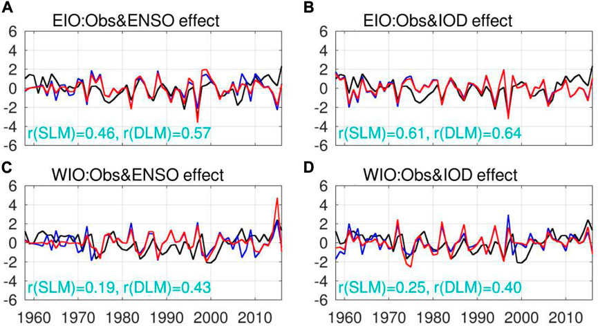
FIGURE 2. Time series of annual mean ORAS4 SSHA (black line), SSHA explained by ENSO index (i.e., NINO3.4 index) using conventional Static Linear Model (SLM; blue line) and Bayesian Dynamic Linear Model (BDLM; red line), for the (A) EIO box, (C) WIO box, shown in Figure 1. Panels b and d are the same as panels (A,C), respectively, but for SSHA explained by the IOD index (i.e., DMI). Specifically, the blue and red lines are the b₁X₁ terms of Eqs 2, 3, respectively, with X₁ being Niño3.4 index for (A), (C) and DMI for (B), (D). The correlations between AVISO observed SSHA and modeled SSHA using SLM (BDLM) are shown at the bottom of each panel. Here all the time series have been normalized by its standard deviation. The standard deviation of EIO, WIO are 2.6 cm and 3.4 cm, respectively.

FIGURE 3

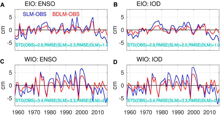
FIGURE 3. Error of SSHA for SLM (blue line) and BDLM (red line) estimation in (A) EIO and (C) WIO region. Panels (B,D) are the same as panels (A,C), respectively, but for IOD contribution. Here the errors are estimated as the deviations of model results from the observation. Or in other words, Error (SLM) = Y(SLM)-OBS and Error (BDLM)=Y(BDLM)-OBS. The standard deviation of the observation and the root mean squared errors of SLM and BDLM results are listed in each panel.

5 The decadal shift of IOD impact before and after 1980s

As discussed in Section 2, the BDLM can measure the time-varying influence of the climate modes, Figure 4 shows the optimized values of the coefficient b₁ in Eq. 2. It should be noted that all four panels of Figure 4 do not represent same time series. In EIO, in particular, the IOD plays a weaker role before 1980s and a stronger influence afterwards in magnitudes (see Figure 4B). In order to see the related processes that may cause this decadal shift in impacts, we calculated regressions of SSTA, precipitation and wind stress onto IOD index for the period of 1958–1979 and 1980–2016 (Figure 5). Weak and strong easterlies in the equatorial Indian Ocean before and after 1980, respectively, are accompanied by differences in atmospheric circulations over the western Pacific and Indian subcontinent. Even though the zonal SST contrast in the equatorial Indian Ocean is assumed to be unity (i.e., discussing regressions onto IOD index), the relatively stronger easterlies along the coastal area of EIO after 1980s drives a relatively stronger upwelling as shown in Figure 4B. In fact, the observed regressions of the autumnal SST in EIO onto the IOD index particularly focusing on the coastal area (95^oW-110^oW, 10^oS-0^o) are −0.48 and −0.66 during the periods 1958–1979 and 1980–2016, respectively, and the difference of these regression values are significant at a 90% confidence limit in F-test.

FIGURE 4

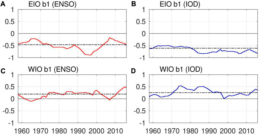
FIGURE 4. Time series of BDLM coefficients, i.e., b1 of Eq. 3, in the EIO (eastern box of Figure 1) for (A) ENSO (red curve), and (B) IOD (blue curve); (C) and (D) are the same as (A) and (B) but for the WIO upwelling region (western box of Figure 1). The horizontal dashed-dotted black line in each panel shows the corresponding SLM coefficient, i.e., b₁ of Eq. 2, which is a constant value.

FIGURE 5

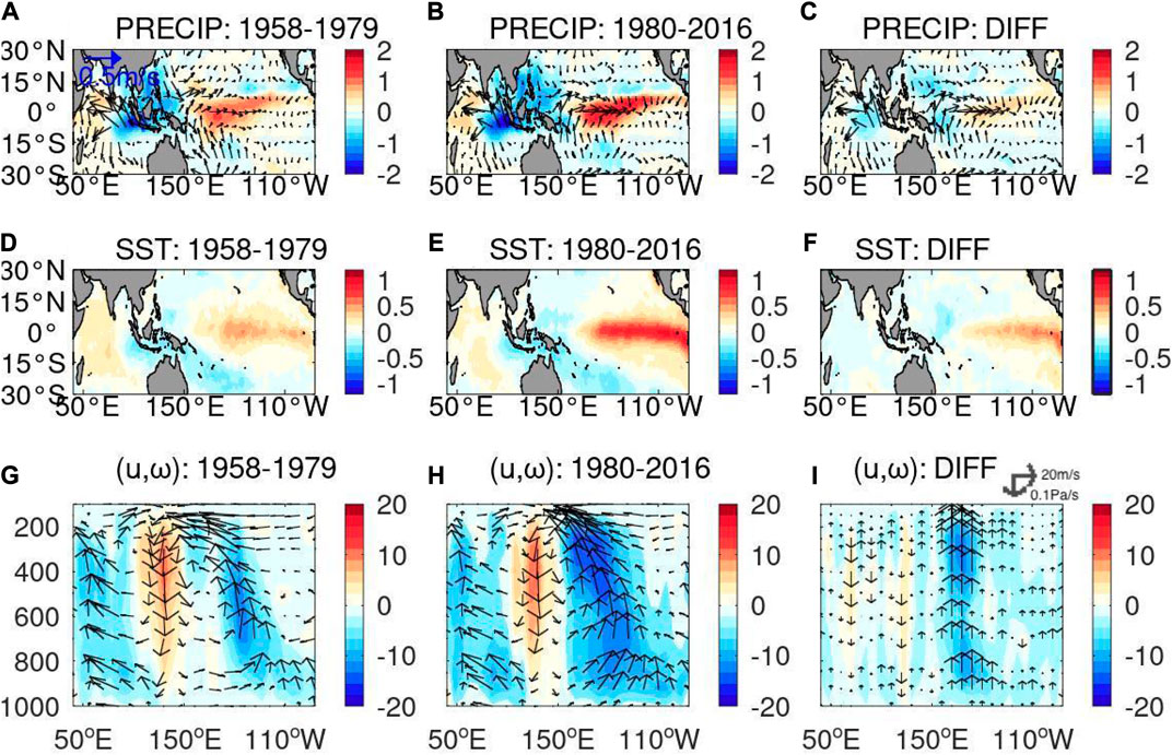
FIGURE 5. Regression onto SON DMI for precipitation (color shading; unit: mm/day) and zonal and meridional winds anomaly at 1000 hPa (vectors; unit: m/s) during the periods (A) 1958–1979 and (B) 1980–2016. (C) Differences of these two periods (i.e., panel b minus panel a). (D–F) The same as (A–C), but for SST (color shading; unit:^oC). (G–I) The same as (A–C), but for the zonal and vertical winds (vectors; unit: m/s and hPa/day, respectively) along the equatorial Ind-Pacific Ocean. Shades represent vertical wind velocity.

These differences are primarily due to the background change of ocean temperature. Figure 6 shows the difference in vertical sections of Indo-Pacific ocean temperature and Walker circulation cell before and after 1980s. After 1980, the strong warming tendency is observed in the surface layer of the whole Indo-Pacific Oceans (Figure 6B) together with the changes in Indo-Pacific Walker circulation (Figure 6A). In particular, this ocean surface warming is accompanied by the strong vertical gradient around the ocean thermocline in the eastern Indian Ocean. As a result, the coastal wind in the eastern Indian Ocean induces the IOD signal more effectively in EIO. The optimized values of the coefficient b₁ represents changes of the efficiency in forming the IOD signal in EIO as an ocean response to the surface wind stress forcing aloft, corresponding to changes of the background states of the Indian ocean. Since the IOD index is defined as zonal contrast of the Indian Ocean SST anomalies, the uniform negative anomaly in the Indian Ocean in Figure 5F suggests that the IOD-related SST anomalies represent the enhancing and reducing tendencies in the EIO and WIO, respectively.

FIGURE 6

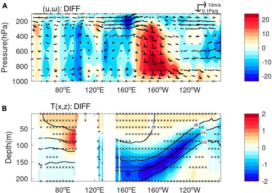
FIGURE 6. (A) The difference of equatorial vertical wind velocity (shade, hPa day⁻¹), and zonal (m s⁻¹) and vertical wind velocity (vectors) along the equatorial Indian Pacific Ocean before and after 1980 (i.e., values after 1980 minus those before 1980). (B) The difference of ocean temperature before and after 1980 (shade, ^oC), and the climatology (bold curves, ^oC). Cross marks represent the significant differences at a 95% confidence limit.

6 Relationship to decadal variability in the tropical Pacific

From Figure 4A, we also found that there is decadal modulation in impacts of ENSO on EIO upwelling, namely, stronger impact between 1976 and 2002 and weaker impact before 1976 and after 2002. The ENSO and IOD impacts on WIO also show similar timeseries (see Figures 4C,D). These values of b₁ are highly correlated with the so-called PDO index (The correlation values relative to the PDO index 9-year running mean applied are −0.71, 0.64 and 0.44 in Figures 4A,C,D, respectively). Note that, for convenience, here we refer to the above three periods as the negative, positive and negative PDO periods, respectively. Thus, the ENSO has stronger and weaker impacts on EIO upwelling during the positive and negative PDO periods, respectively. Consistent with this BDLM result, the observed regressions of SST in EIO onto the NINO3.4 index represent the significantly larger value in magnitude in the positive PDO period than in the negative PDO period at a 95% confidence limit. We examine the related processes by discussing the differences of regressions in the positive and negative PDO periods as below (Figure 7). Besides, the composite maps (i.e., the background states) represent the PDO-like patterns (Figure 8). The convective activity in the atmosphere is reduced largely over the western Pacific Ocean as a part of the weak Walker circulation (Figure 8A), corresponding to warm upper ocean in the eastern Pacific Ocean (Figure 8B). In contrast to Figure 6B, the composite maps (i.e., the background states) hardly show significant differences in the upper ocean temperature of the Indian Ocean.

FIGURE 7

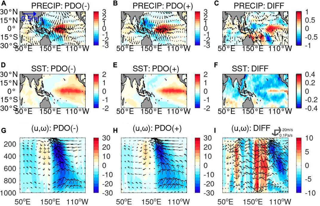
FIGURE 7. Regression onto NDJ ENSO index for precipitation (color shading; unit: mm/day) and surface winds (vectors: m/s) during (A) negative and (B) positive PDO periods. (C) The difference of these two periods [i.e., panel (B) minus panel (A)]. (D–F) The same as (A–C), but for SST (color shading; unit: ^oC). (G–I) The same as (A–C), but for the zonal and vertical winds (vectors; units: m/s and hPa/day, respectively) along the equatorial Ind-Pacific Ocean. Shades represent vertical wind velocity.

FIGURE 8

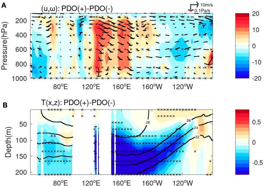
FIGURE 8. Same as Figure 6, but for the difference of (A) vertical velocity (shaded, hPa/day) and zonal (m s⁻¹, vector) and temperature (shading) averaged along the equatorial Indian- Pacific Ocean during positive and negative PDO periods. The negative PDO periods are defined as 1958–1976 and 2002–2016, and the positive PDO period is defined as 1976–2002. The climatology of ocean temperature (bold curves, ^oC) is superimposed in panel (B). Cross marks represent the significant differences at a 95% confidence limit.

We further plot the regression of SSTA, precipitation and wind forcing onto ENSO index during the above defined positive and negative PDO periods (see Figure 7). Even though we always use NINO3.4 index to define the ENSO events, the observed SST anomaly in the eastern Pacific Ocean is slightly shifted eastward in the positive PDO period (Figure 7F). In other words, during the positive and negative PDO periods, the spatial patterns of SST anomaly in a background state are similar to the so-called Eastern Pacific (EP) and Central Pacific (CP) El Nino events, respectively. This is further related to stronger easterly wind along the equatorial Indian Ocean during the positive PDO phase and will drive stronger upwelling in the WIO boxed region. Some studies indicated that EP El Nino events can be more frequently observed in the positive PDO period (Feng et al., 2019), when using two widely used El Nino classification methods: the so-called NINO method (Kug et al., 2009) and the El Nino Modoki index (Ashok et al., 2007). Both the methods define 1 EP (1972/73) and 1CP (1968/69) events during 1958–1975, 4 EP (1976/77, 1982/83, 1986/87, and 1997/98) and 2 CP (1977/78, and 1994/95) events during 1976–2001 and 2 EP (2006/07, and 2014/15) and 3 CP (2002/03, 2004/05, and 2009/10) events during 2002–2016 (e.g., Table 1 in Feng et al., 2019). Note that 2 El Nino events for each of the periods during 1958–1975 and during 1976–2001 are inconsistently classified by the above two methods. This suggests that during the positive PDO period, there are relatively more EP El Nino events, which may lead to stronger equatorial easterly wind in the Indian Ocean, which will further drive stronger upwelling in the WIO. The optimized value of the coefficient b₁ seems to represent changes of ENSO impact primarily due to the distinct ENSO flavor associated with the changes in the background states. The observed regressions of the wintertime SST in central equatorial Pacific (NINO4 region; 160^oE-150^oW, 5^oS-5^oN) onto the NINO index (NINO3.4 index in this study) are 0.57 and 0.71 during the positive and negative PDO periods, respectively. The difference of the regression values of NINO4 SST is significant at a 95% confidence limit, also suggesting the relatively weak contribution of CP El Nino in the positive PDO period.

7 Conclusion and discussion

In this paper, the decadal modulations of ENSO and IOD impacts on the tropical Indian Ocean upwelling are explored by combining the observational data since 1958 and statistical model. The BDLM enables us to demonstrate temporal variations of the contributions of ENSO and IOD by optimizing regression coefficients, thereby showing superiority to the SLM in reproducing the upwelling tendency. We found that the optimized values in the regression coefficients contribute to representing the effects of decadal variations of the background climate states that can modulate the strength of the Indian Ocean upwelling. For example, there is a decadal shift of IOD impact before and after 1980s for the EIO upwelling. This is mainly caused by the shift of wind stress forcing along the eastern coast in magnitudes, corresponding to the changes in sensitivity of the ocean response to atmospheric forcing in relation to the strength of upper ocean stratification (Section 5). The impacts of ENSO on EIO upwelling (and the ENSO and IOD impacts on WIO upwelling) is also modulated on decadal timescales, and the impact is stronger during the period of 1976–2002. Our analysis shows that this is mainly caused by the stronger easterly wind along the equatorial Indian Ocean, dependent on the distinct ENSO flavors dominantly observed in a specific decade (Section 6). Thus, the optimized regression coefficients in BDLM improve the Indian Ocean upwelling particularly on decadal timescales, by reflecting the decadal changes in the Indian Ocean response (i.e., stratification) as in Section 5 and probably in the Pacific Ocean forcing (i.e., ENSO flavor) as in Section 6.

Note here, our results are based on static linear regression model and the Bayesian dynamic linear model, as discussed in Zhang and Han (2020). Thus, the contribution of oceanic waves is not directly estimated but implicitly taken into account in defining regression values in a statistical sense. Since the oceanic wave also plays an important role when moving westward, advanced estimates of its contribution can be a topic for future research. In addition, the upwelling as a response of the ocean to wind stress forcing can represent feedback to wind stress. While, logically speaking, the contribution of this feedback can be grossly represented in our estimation, the detailed coupled processes of atmosphere and ocean are still unclear. Direct verification of coupled climate process modulating the ocean upwelling is also an interesting research questions for future works. Nevertheless, we have built on Zhang and Han (2020), in which they mainly focused on the ocean upwelling on interannual time scales, by showing some important processes that primarily effect on the modulation of the impact of climate modes on decadal timescales. Our results also suggest that the different types of El Nino and the changing atmosphere-ocean state in the climate models towards precise simulations of the impact of climate modes on the Indian Ocean upwelling.

Data availability statement

The original contributions presented in the study are included in the article/Supplementary Material, further inquiries can be directed to the corresponding authors.

Author contributions

XZ and TM proposed the research direction. TM specified the research target. All authors analyzed the data, created figures, discussed the research results, and wrote the manuscript. All authors contributed to the article and approved the submitted version.

Acknowledgments

We gratefully acknowledge funding from the Japan Society for the Promotion of Science (JSPS) KAKENHI (JP19H05703) and the MEXT project (JPMXD0722680395), and the discussions with Prof. Tomoki Tozuka for his significant improvements to our work. Thanks are also due to Prof. Weiqing Han for her supports to perform the linear model estimations.

Conflict of interest

The authors declare that the research was conducted in the absence of any commercial or financial relationships that could be construed as a potential conflict of interest.

Publisher’s note

All claims expressed in this article are solely those of the authors and do not necessarily represent those of their affiliated organizations, or those of the publisher, the editors and the reviewers. Any product that may be evaluated in this article, or claim that may be made by its manufacturer, is not guaranteed or endorsed by the publisher.

Supplementary material

The Supplementary Material for this article can be found online at: https://www.frontiersin.org/articles/10.3389/feart.2023.1212421/full#supplementary-material

References

Annamalai, H., Liu, P., and Xie, S.-P. (2005). Southwest Indian Ocean SST variability: its local effect and remote influence on Asian monsoons. J. Clim. 18, 4150–4167. doi:10.1175/JCLI3533.1

CrossRef Full Text | Google Scholar

Ashok, K., Chan, W. L., Motoi, T., and Yamagata, T. (2004). Decadal variability of the Indian Ocean dipole. Geophys. Res. Lett. 31, L24207. doi:10.1029/2004GL021345

CrossRef Full Text | Google Scholar

Ashok, K. S. B., Rao, A. S., Weng, H., and Yamagata, T. (2007). El Nino Modoki and its teleconnection. J. Geophys. Res., doi:10.1029/2006JC003798

CrossRef Full Text | Google Scholar

Balmaseda, M. A., Trenberth, K. E., and Källén, E. (2013). Distinctive climate signals in reanalysis of global ocean heat content. Geophys. Res. Lett. 40, 1754–1759. doi:10.1002/grl.50382

CrossRef Full Text | Google Scholar

Baquero-Bernal, A., and Latif, M. (2005). Wind-driven oceanic Rossby waves in the tropical south Indian ocean with and without an active ENSO. J. Phys. Oceanogr. 35, 729–746. doi:10.1175/jpo2723.1

CrossRef Full Text | Google Scholar

Birol, F., and Morrow, R. (2001). Source of the baroclinic waves in the southeast Indian Ocean. J. Geophys. Res. 106, 9145–9160. doi:10.1029/2000JC900044

CrossRef Full Text | Google Scholar

Chambers, D. P., Tapley, B. D., and Stewart, R. H. (1999). Anomalous warming in the Indian ocean coincident with El Niño. J. Geophys. Res. 104, 3035–3047. doi:10.1029/1998jc900085

CrossRef Full Text | Google Scholar

Chen, G., Han, W., Li, Y., and Wang, D. (2016). Interannual variability of equatorial eastern Indian Ocean Upwelling: local versus remote forcing. J. Phys. Oceanogr. 46, 789–807. doi:10.1175/JPO-D-15-0117.1

CrossRef Full Text | Google Scholar

Deepa, J. S., Gnanaseelan, C., Kakatkar, R., Parekh, A., and Chowdary, J. S. (2018). The interannual sea level variability in the Indian Ocean as simulated by an Ocean General Circulation Model. Int. J. Climatol. 38, 1132–1144. doi:10.1002/joc.5228

CrossRef Full Text | Google Scholar

Feng, J., Lian, T., Ying, J., Li, J., and Li, G. (2019). Do CMIP5 models show El Nino diversity? J. Clim. 33, 1619–1641. doi:10.1175/jcli-d-18-0854.1

CrossRef Full Text | Google Scholar

Fu, L. L., and Smith, R. D. (1996). Global ocean circulation from satellite altimetry and high resolution computer simulation. Bull. Amer. Meteor. Soc. 77, 2625–2636. doi:10.1175/1520-0477(1996)077<2625:gocfsa>2.0.co;2

CrossRef Full Text | Google Scholar

Gnanaseelan, C., and Vaid, B. H. (2010). Interannual variability in the biannual Rossby waves in the tropical Indian Ocean and its relation to Indian Ocean Dipole and El Niño forcing. Clim. Dyn. 60, 27–40. doi:10.1007/s10236-009-0236-z

CrossRef Full Text | Google Scholar

Han, W., Meehl, G., Stammer, D., Hu, A., Hamlington, B., Kenigson, J., et al. (2017). Spatial patterns of sea level variability associated with natural internal climate modes. Surv. Geophys. 38 (1), 217–250. doi:10.1007/s10712-016-9386-y

PubMed Abstract | CrossRef Full Text | Google Scholar

Han, W., Stammer, D., Meehl, G. A., Hu, A., Sienz, F., and Zhang, L. (2018). Multi-decadal trend and decadal variability of the regional sea level over the Indian ocean since the 1960s: roles of climate modes and external forcing. Climate 6 (2), 51–356. doi:10.3390/cli6020051

CrossRef Full Text | Google Scholar

Han, W., and Webster, P. J. (2002). Forcing mechanisms of sea-level interannual variability in the Bay of bengal. J. Phys. Oceanogr. 32, 216–239. doi:10.1175/1520-0485(2002)032<0216:fmosli>2.0.co;2

CrossRef Full Text | Google Scholar

Hermes, J. C., and Reason, C. J. C. (2008). Annual cycle of the South Indian Ocean (Seychelles-Chagos) thermocline ridge in a regional ocean model. J. Geophys. Res. 113, C04035. doi:10.1029/2007JC004363

CrossRef Full Text | Google Scholar

Hu, S., Zhang, Y., Feng, M., Du, Y., Sprintall, J., Wang, F., et al. (2019). Interannual to decadal variability of upper-ocean salinity in the southern Indian Ocean and the role of the Indonesian Throughflow. J. Clim. 32, 6403–6421. doi:10.1175/JCLI-D-19-0056.1

CrossRef Full Text | Google Scholar

Huang, B., and Kinter, J. L. (2002). Interannual variability in the tropical Indian Ocean. J. Geophys. Res. 107, 3199. doi:10.1029/2001JC001278

CrossRef Full Text | Google Scholar

Izumo, T., Vialard, J., Lengaigne, M., Montegut, C. D., Behera, S. K., Luo, J. J., et al. (2010). Influence of the state of the Indian Ocean Dipole on the following year's El Niño. Nat. Geosci. 3, 168–172. doi:10.1038/Ngeo760

CrossRef Full Text | Google Scholar

Jury, M. R., and Huang, B. (2004). The Rossby wave as a key mechanism of Indian Ocean climate variability. Deep Sea Res. Part I Oceanogr. Res. Pap. 51, 2123–2136. doi:10.1016/j.dsr.2004.06.005

CrossRef Full Text | Google Scholar

Kalnay, E., Kanamitsu, M., Kistler, R., Collins, W., Deaven, D., Gandin, L., et al. (1996). The NCEP/NCAR 40-year reanalysis project. Bull. Am. Meteorological Soc. 77, 437–471. doi:10.1175/1520-0477(1996)077<0437.TNYRP.>2.0.CO;2

CrossRef Full Text | Google Scholar

Krishnaswamy, J., Vaidyanathan, S., Rajagopalan, B., Bonell, M., Sankaran, M., Bhalla, R. S., et al. (2015). Non-stationary and non-linear influence of ENSO and Indian Ocean Dipole on the variability of Indian monsoon rainfall and extreme rain events. Clim. Dyn. 45, 175–184. doi:10.1007/s00382-014-2288-0

CrossRef Full Text | Google Scholar

Kug, J.-S., Jin, F.-F., and An, S.-I. (2009). Two types of El Niño events: cold tongue El Niño and warm pool El Niño. J. Clim. 22, 1499–1515. doi:10.1175/2008jcli2624.1

CrossRef Full Text | Google Scholar

Kumar, K. K., Rajagopalan, B., and Cane, M. A. (1999). On the weakening relationship between the Indian monsoon and ENSO. Science 284, 2156–2159. doi:10.1126/science.284.5423.2156

PubMed Abstract | CrossRef Full Text | Google Scholar

Levitus, S., Antonov, J. I., Boyer, T. P., Baranova, O. K., Garcia, H. E., Locarnini, R. A., et al. (2012). World ocean heat content and thermosteric sea level change (0–2000 m). Geophys. Res. Lett. 39, 1955–2010. doi:10.1029/2012gl051106

CrossRef Full Text | Google Scholar

Masumoto, Y., and Meyers, G. (1998). Forced Rossby waves in the southern tropical Indian Ocean. J. Geophys. Res. 103, 27589–27602. doi:10.1029/98jc02546

CrossRef Full Text | Google Scholar

McCreary, J. P., Kundu, P. K., and Molinari, R. L. (1993). A numerical investigation of dynamics, thermodynamics and mixed-layer processes in the Indian Ocean. Prog. Oceanogr. 31, 181–244. doi:10.1016/0079-6611(93)90002-U

CrossRef Full Text | Google Scholar

Murtugudde, R., McCreary, J. P., and Busalacchi, A. J. (2000). Oceanic processes associated with anomalous events in the Indian Ocean with relevance to 1997-1998. J. Geophys. Res. 105, 3295–3306. doi:10.1029/1999jc900294

CrossRef Full Text | Google Scholar

Murtugudde, R., Signorini, S., Christian, J., Busalacchi, A., McClain, C., and Picaut, J. (1999). Ocean color variability of the tropical Indo-Pacific basin observed by SeaWiFS during 1997-1998. J. Geophys. Res. 104, 18351–18366. doi:10.1029/1999jc900135

CrossRef Full Text | Google Scholar

Périgaud, C., and Delecluse, P. (1992). Annual Sea level variations in the southern tropical Indian ocean from geosat and shallow-water simulations. J. Geophys. Res. 97, 20169–20178. doi:10.1029/92JC01961

CrossRef Full Text | Google Scholar

Périgaud, C., and Delecluse, P. (1993). Interannual Sea level variations in the tropical Indian ocean from geosat and shallow water simulations. J. Phys. Oceanogr. 23, 1916–1934. doi:10.1175/1520-0485(1993)023<1916:islvit>2.0.co;2

CrossRef Full Text | Google Scholar

Petris, G. (2010). dlm: bayesian and likelihood analysis of dynamic linear models. r package version 1.1-1. http://CRAN. R-project.org/package5dlm.

Google Scholar

Petris, G., Petrone, S., and Campagnoli, P. (2009). Dynamic linear models with R. New York, NY, USA: Springer Verlag, 31–84.

CrossRef Full Text | Google Scholar

Potemra, J. T. (2001). Contribution of equatorial Pacific winds to southern tropical Indian Ocean Rossby waves. J. Geophys. Res. 106, 2407–2422. doi:10.1029/1999jc000031

CrossRef Full Text | Google Scholar

R Development Core Team (2016).R: A language and environment for statistical computing Vienna, Austria: R Foundation for Statistical Computing.

Google Scholar

Rao, S. A., and Behera, S. K. (2005). Subsurface influence on SST in the tropical Indian Ocean: structure and interannual variability. Dyn. Atmos. Oceans 39, 103–135. doi:10.1016/j.dynatmoce.2004.10.014

CrossRef Full Text | Google Scholar

Rayner, N. A., Parker, D. E., Horton, E. B., Folland, C. K., Alexander, L. V., Rowell, D. P., et al. (2003). Global analyses of sea surface temperature, sea ice, and night marine air temperature since the late nineteenth century. J. Geophys. Res. 108, 4407. doi:10.1029/2002JD002670

CrossRef Full Text | Google Scholar

Saji, N. H., Goswami, B. N., Vinayachandran, P. N., and Yamagata, T. (1999). A dipole mode in the tropical Indian Ocean. Nature 401 (6751), 360–363. doi:10.1038/43854

PubMed Abstract | CrossRef Full Text | Google Scholar

Schott, F. A., Xie, S.-P., and McCreary, J. P. (2009). Indian Ocean circulation and climate variability. Rev. Geophys. 47, RG1002. doi:10.1029/2007RG000245

CrossRef Full Text | Google Scholar

Shinoda, T., Hendon, H. H., and Alexander, M. A. (2004). Surface and subsurface dipole variability in the Indian Ocean and its relation with ENSO. Deep Sea Res. Part I 51, 619–635. doi:10.1016/j.dsr.2004.01.005

CrossRef Full Text | Google Scholar

Susanto, R. D., Gordon, A. L., and Zheng, Q. N. (2001). Upwelling along the coasts of Java and Sumatra and its relation to ENSO. Geophys. Res. Lett. 28, 1599–1602. doi:10.1029/2000gl011844

CrossRef Full Text | Google Scholar

Tozuka, T., Yokoi, T., and Yamagata, T. (2010). A modeling study of interannual variations of the Seychelles Dome. J. Geophys. Res. 115, C04005. doi:10.1029/2009JC005547

CrossRef Full Text | Google Scholar

Trenary, L., and Han, W. (2012). Intraseasonal to interannual variability of South Indian Ocean sea level and thermocline: remote versus local forcing. J. Phys. Oceanogr. 42, 602–627. doi:10.1175/jpo-d-11-084.1

CrossRef Full Text | Google Scholar

Wang, L., Koblinsky, C. J., and Howden, S. (2001). Annual Rossby wave in the Southern Indian Ocean: why does it “appear” to break down in the middle ocean? J. Phys. Oceanogr. 31, 54–74. doi:10.1175/1520-0485(2001)031<0054:arwits>2.0.co;2

CrossRef Full Text | Google Scholar

White, W. B. (2000). Evidence for coupled Rossby waves in the annual cycle of the Indo-Pacific ocean. J. Phys. Oceanogr. 31, 2944–2957. doi:10.1175/1520-0485(2001)031<2944:efcrwi>2.0.co;2

CrossRef Full Text | Google Scholar

Woodberry, K. E., Luther, M. E., and O’Brien, J. J. (1989). The wind-driven seasonal circulation in the southern tropical Indian ocean. J. Geophys. Res. 94 (17), 17985–18018. doi:10.1029/JC094Ic12P17985

CrossRef Full Text | Google Scholar

Xie, S.-P., Annamalai, H., Schott, F. A., and McCreary, J. P. (2002). Structure and mechanisms of south Indian ocean climate variability. J. Clim. 15, 864–878. doi:10.1175/1520-0442(2002)015<0864:samosi>2.0.co;2

CrossRef Full Text | Google Scholar

Xie, S.-P., and Arkin, P. A. (1996). Analyses of global monthly precipitation using gauge observations, satellite estimates, and numerical model predictions. J. Clim. 9, 840–858. doi:10.1175/1520-0442(1996)009<0840:aogmpu>2.0.co;2

CrossRef Full Text | Google Scholar

Xie, S.-P., and Arkin, P. A. (1997). Global precipitation: A 17-year monthly analysis based on gauge observations, satellite estimates, and numerical model outputs. Bull. Amer. Meteor. Soc. 78, 2539–2558. doi:10.1175/1520-0477(1997)078<2539:gpayma>2.0.co;2

CrossRef Full Text | Google Scholar

Xie, S.-P., Du, Y., Huang, G., Zheng, X.-T., Tokinaga, H., Hu, K., et al. (2010). Decadal shift in El Niño influences on indo-western pacific and East asian climate in the 1970s. J. Clim. 23, 3352–3368. doi:10.1175/2010jcli3429.1

CrossRef Full Text | Google Scholar

Yang, J., Yu, L., Koblinsky, C. J., and Adamec, D. (1998). Dynamics of the seasonal variations in the Indian Ocean from TOPEX/POSEIDON sea surface height and an ocean model. Geophys. Res. Lett. 25, 1915–1918. doi:10.1029/98GL01401

CrossRef Full Text | Google Scholar

Yokoi, T., Tozuka, T., and Yamagata, T. (2008). Seasonal variation of the Seychelles dome. J. Clim. 21, 3740–3754. doi:10.1175/2008jcli1957.1

CrossRef Full Text | Google Scholar

Yokoi, T., Tozuka, T., and Yamagata, T. (2009). Seasonal variations of the Seychelles dome simulated in the CMIP3 models. J. Phys. Oceanogr. 39, 449–457. doi:10.1175/2008JPO3914.1

CrossRef Full Text | Google Scholar

Yu, W., Xiang, B., Liu, L., and Liu, N. (2005). Understanding the origins of interannual thermocline variations in the tropical Indian Ocean. Geophys. Res. Lett. 32, L24706. doi:10.1029/2005GL024327

CrossRef Full Text | Google Scholar

Zhang, X., and Han, W. (2020). Effects of climate modes on interannual variability of upwelling in the tropical Indian ocean. J. Clim. 33, 1547–1573. doi:10.1175/JCLI-D-19-0386.1

CrossRef Full Text | Google Scholar

Zhang, X., and Mochizuki, T. (2022). Sea surface height fluctuations relevant to Indian summer monsoon over the northwestern Indian Ocean. Front. Clim. 4, 1008776. doi:10.3389/fclim.2022.1008776

CrossRef Full Text | Google Scholar

Zhuang, W., Feng, M., Du, Y., Schiller, A., and Wang, D. (2013). Low-frequency sea level variability in the southern Indian Ocean and its impacts on the oceanic meridional transports. J. Geophys. Res. Oceans 118, 1302–1315. doi:10.1002/jgrc.20129

CrossRef Full Text | Google Scholar