Improving mass change estimation in Panama with the GRACE/GFO gravity field using the variational mode decomposition

In this study, we aim to estimate the mass changes in Panama using the Gravity Recovery and Climate Experiment level-2 products, which are formed as spherical harmonic coefficients and limited by stripe noise. The empirical de-striping method and the temporal filter achieved by empirical mode decomposition can be used to reveal the signals but are still limited in signal reservation and noise reduction. To this end, we put forward a novel efficient strategy that uses the variational mode decomposition algorithm to filter the time series of each SHC separately. Based on the two reliable mascon products and in situ short-term groundwater observations, various comparisons in spatial, spectral, and temporal domains are implemented. In addition, the SNR (signal-to-noise ratio) index and the three-cornered hat method are adopted for assessment. The main results and conclusions are as follows: 1) Our filter outperforms the two previous methods with the best SNR (2.14) and the lowest Panama regional uncertainty (70 mm) for all available months. 2) Our estimate of the basin groundwater storage is closest to one of the groundwater observations with the maximum correlation coefficient (0.72, p<0.05). This result suggests that our method seems to detect small-scale mass signals that are undetectable in the two mascon products. Our work provides a reference for studying the mass change of small-scale basins in low latitudes.

1 Introduction

Since the launch of the Gravity Recovery and Climate Experiment (GRACE) satellite mission, GRACE (2002–2017) and GRACE Follow-On (GFO) (2018–present) have produced extremely precise measurements of the larger-scale temporal gravity of the Earth system (Swenson and Wahr, 2002). Observing the mass variations in the atmosphere, hydrosphere, ocean, and cryosphere has been made possible by the GRACE/GFO mission (Nerem et al., 2003; Ray and Ponte, 2003; Swenson et al., 2003; King and Padman, 2005). Practically, the Earth’s mass transports are quantified using the gravity field models, which are represented as a collection of spherical harmonic coefficients (SHCs) (Chen Q. et al., 2021).

Due to the GRACE/GFO orbit or aliasing error, an irrational correlation exists among the SHCs of specific degrees (odd or even) within a given order (Swenson and Wahr, 2006). As a result, all the unrestrained inversion results converted from SHC products are seriously contaminated by north-south stripe noise. To this end, the post-processing method is necessary.

The spatial filter, such as the Gaussian, Han, and Fan filters, can be employed to filter the data. However, it is worth noting that they may underestimate the geophysical signals (Wahr et al., 1998; Han et al., 2005; Chen et al., 2006; Sasgen et al., 2006; Klees et al., 2008b; Zhang et al., 2009; Pu et al., 2022). To address this, considering the pattern of stripe noise in the spatial domain, Swenson and Wahr (2006) proposed the empirical de-striping method that seeks the pattern using a moving window quadratic polynomial. Afterward, the PnMl method, which is widely utilized, is a development of this method (Klees et al., 2008a; Chen et al., 2008; Duan et al., 2009; Chambers and Bonin, 2012). Nonetheless, the further application of these empirical de-striping methods is mainly constrained by two factors: 1) the insufficient filtering in high-order SHCs (resulting in abundant stripe noise) due to the inadequate observation of SHCs for the fitting function and 2) the potential distortion of the geophysical signal.

In contrast, the temporal filter ensures temporal information reservation since these filters treat the stripe noise as random noise and suggest that this can be identified with time information (prior information or statistical properties). This property correspondingly leads to a high requirement for computational operation, for instance, the Kalman filter (Zaitchik et al., 2008), principal component analysis (Crossley et al., 2005; Rangelova et al., 2007), and so on (Wang et al., 2016; Shen et al., 2021).

To end this, Huan et al. (2022) proposed a simple and efficient technique that adopts the Empirical Mode Decomposition (EMD) to decompose the time series of each SHC separately (Huan et al., 2022). Unlike the complexity and extensive workload of the previous temporal filter, this method treats each SHC individually, considering the orthogonality of basic functions. However, EMD is known for limitations like sensitivity to noise and sampling, boundary issues, and mode aliasing (Dragomiretskiy and Zosso, 2014). These issues can be improved by the Variational Mode Decomposition (VMD) proposed by Dragomiretskiy and Zosso (2014), which can extract, concurrently, the desired mode with an independent center frequency.

Consequently, in this study, we propose a new strategy that employs the VMD to filter the time series of SHCs. Our filter is expected to improve the estimates of the mass change in Panama (Figure 1), which is our objective. In the study, we investigate the result of our filter in the spatial, spectral, and temporal domains stepwise. Afterward, our filter is assessed by the SNR (signal-to-noise ratio) index and the three-cornered hat technique. In the end, our filter is adopted to estimate the mass changes in Panama, which are analyzed by independent observations.

FIGURE 1

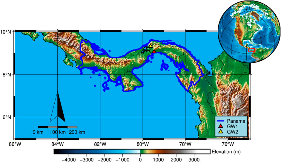
FIGURE 1. Map of Panama. The triangles denote the in situ groundwater observations.

2 Study area and materials

2.1 Study area

Panama mostly lies within 7°N∼10°N and 77°W∼83°W (Figure 1) and is an intercontinental nation that straddles both southern South America and northern North America. Panama shares borders with Colombia to the southeast, the Caribbean Sea to the north, the Pacific Ocean to the south, and Costa Rica to the west. Panama has a tropical climate (Beck et al., 2018). In Panama, temperatures are uniformly high with little seasonal variations and the rainy season typically lasts from April to December but can last anywhere between seven and 9 months. The terrain in Panama is primarily characterized by highlands, with only narrow coastal plains. Nearly 500 rivers wind through Panama’s rugged landscape. Most are not navigable and many originate from turbulent highland creeks, meandering through valleys and forming coastal deltas.

2.2 GRACE/GFO products

The estimates of global mass field (2002.04–2021.04) are based on GRACE/GFO Release 06 GSM products (the SHCs truncated at 60°) provided by three Scientific Data Centers, the Center for Space Research (CSR) at the University of Texas in Austin, Geoforschungs Zentrum Potsdam (GFZ), and the Jet Propulsion Laboratory (JPL). Firstly, the conventional treatments in low-degree terms are implemented: the degree one and the C₂₀/C₃₀ terms, which represent the changes in the geo-center and the oblate shape of the geopotential, respectively. The two terms were replaced by the observation of satellite laser ranging (Swenson et al., 2008) and the combination of GRACE/GFO observation and ocean models (Cheng et al., 2013; Loomis et al., 2020), respectively. Afterward, the monthly residual SHCs are anomalies that have deviated from the GRACE/GFO mean gravity field (2004–2010). Additionally, the glacial isostatic adjustment correction is executed by the ICE-6G_D model (Peltier et al., 2018), which is given as trends of SHCs per year and transformed into equivalent monthly corrections that have deviated from the above baseline (Ferreira et al., 2023). Eventually, aiming to reduce the noise in the SHCs (Chambers and Bonin, 2012), our following work is mainly based on the average estimates of three Scientific Data Centers (CSR, GFZ, and JPL).

Furthermore, two official GRACE/GFO mascon products (gridded mass field) are implemented as reliable estimates to directly assess our results (Save et al., 2016; Wiese et al., 2016): 1) CSR mascon RL06 v2 and 2) JPL mascon RL06 v2. All the technical treatments for the mascon product are kept with the GSM product, except for the minor impact from ellipsoid corrections in low latitudes (Li et al., 2017). To reduce leakage error along the coastlines, a Coastline Resolution Improvement filter is employed in the JPL mascon product.

2.3 Auxiliary materials

Aiming to indirectly assess our estimates, the rest of the auxiliary data are adopted to investigate the groundwater storage (GWS) changes in Panama. To end this, the monthly soil moisture storages need to be utilized, which is collected from the Global Land Data Assimilation System NOAH Version 2.1 model (Rodell et al., 2004; Syed et al., 2008). In addition, two short-term groundwater observations, namely, GW1 and GW2 (Figure 1) are digitally extracted from the previous study (Sprenger et al., 2013; Gonzalez-Valoys et al., 2022).

3 Methods

3.1 The global mass field

The monthly SHCs are converted into the global mass field Δh in terms of equivalent water height (EWH) (Wahr et al., 1998):

$\Delta \mathrm{h}\left(\mathrm{\theta },\mathrm{\lambda }\right)=\frac{\mathrm{R}{\mathrm{\rho }}_{\mathrm{e}}}{3{\mathrm{\rho }}_{\mathrm{w}}}{\displaystyle \sum _{n={\mathrm{n}}_{start}=0}^{{\mathrm{n}}_{end}=60}}\frac{2\mathrm{n}+1}{1+{\mathrm{k}}_{\mathrm{n}}}{\displaystyle \sum _{\mathrm{m}=0}^{\mathrm{n}}}{\mathrm{P}}_{\mathrm{n}\mathrm{m}}\left(\cos \mathrm{\theta }\right){\mathrm{W}}_{\mathrm{n}\mathrm{m}}\times \left[\Delta {\mathrm{C}}_{\mathrm{n}\mathrm{m}}\cos \left(\mathrm{m}\mathrm{\lambda }\right)+\Delta {\mathrm{S}}_{\mathrm{n}\mathrm{m}}\sin \left(\mathrm{m}\mathrm{\lambda }\right)\right](1)$

where n and m represent degree and order, respectively. θ and λ are the co-latitude and longitude, respectively. R and ρ_e are the equatorial radius and density, respectively. ρ_w is the freshwater density. P_nm, k_n, and W_nm denote the normalized Legendre functions, the load Love numbers, and the spatial smoothing function, respectively. In addition, the pattern per degree of the mass field in the spectral domain can be investigated by the signal variance σ_n:

${\sigma }_n=\sqrt[2]{{\displaystyle \sum _{m=0}^n}\left({\Delta \mathrm{C}}_{nm}^2+{\Delta \mathrm{S}}_{nm}^2\right)}(2)$

3.2 The empirical de-striping method

The original mass fields are contaminated by north-south stripe noise, which is linked to the correlated errors in the SHCs (i.e., spurious correlations between specific ΔC_nm/ΔS_nm). To this end, researchers used the PnMl method (Chen et al., 2008; Chen et al., 2017). The P4M6 method treats all ΔC_nm/ΔS_nm with the same m as a series. For each m from 6 to 50 with the same parity of n, this method removes the correlated error for the original ΔC_nm/ΔS_nm. The mathematical model of the P4M6 method is as follows:

${\Delta \mathrm{C}}_{lm}^{\mathrm{c}\mathrm{o}\mathrm{r}}={\displaystyle \sum _{i=0}^p}\left[{\displaystyle \sum _{j=0}^p}{\left({\displaystyle \sum _{\begin{array}{c}n=l_{\mathit{min}}\\ n:evenorodd\end{array}}^{l_{\mathit{max}}}}{n}^i{n}^j\right)}^{-1}{\displaystyle \sum _{\begin{array}{c}n=l_{\mathit{min}}\\ n:evenorodd\end{array}}^{l_{\mathit{max}}}}{n}^j\Delta {\mathrm{C}}_{\mathrm{n}\mathrm{m}}\right]l^i(3)$

where ${\Delta \mathrm{C}}_{lm}^{\mathrm{c}\mathrm{o}\mathrm{r}}$ denotes the correlated error in $\Delta {\mathrm{C}}_{\mathrm{l}\mathrm{m}}$ for a given degree and order m. $p$ is four in the P4M6 method. $l_{\mathit{max}}$ and $l_{\mathit{min}}$ represent the maximum and minimum degrees in a series for a given order, respectively. The detection of ${\Delta \mathrm{S}}_{lm}^{\mathrm{c}\mathrm{o}\mathrm{r}}$ is similar to this model.

3.3 The algorithm of EMD and VMD

The EMD is an adaptive approach for extracting the signal from the noisy time series $y\left(t\right)$. This method decomposes a time series into a series of Intrinsic Mode Functions ($IMFs$) and a residual component ($res$) (Huang et al., 1998):

$y\left(t\right)={\displaystyle \sum _{i=1}^K}{IMF}_i+res(4)$

where $t$ denotes time. $K$ is the number of IMFs. IMF is defined by two basic conditions with the practical meaning of physical signal: 1) the difference in number between extreme and zero-crossing must be within zero or one. 2) The upper and lower envelopes exhibit local symmetry to the time axis.

The algorithm of EMD is as follows:

1) Extracting local extrema (maximum and minimum values) of the original series $y\left(t\right)$, which is used to fit the upper and lower envelope by a cubic spline function.

2) Subtracting the average value of the two envelopes from $y\left(t\right)$ to obtain a new time series $h\left(t\right)$.

3) Checking whether $h\left(t\right)$ meets the necessary definition of IMF. In practice, the second condition is difficult to meet and empirically replaced by a threshold $SD$ (0.2–0.3):

$SD={\displaystyle \sum _{t=1}^N}\left[\frac{{\left|d_{k+1}\left(t\right)-d_k\left(t\right)\right|}^2}{d_{k-1}^2\left(t\right)}\right](5)$

where $d_k\left(t\right)$ denotes $h\left(t\right)$ in the kth iteration. N is the length of the original series.

4) Repeating the above sifting procedure (i.e., steps 1–3) in $h\left(t\right)$ if $h\left(t\right)$ cannot meet the condition. If $h\left(t\right)$ meets the condition, $h\left(t\right)$ is selected as an IMF and removed from the original series to get a residue.

5) Repeating the iteration (i.e., steps 1–4) in the residue until all the IMF is obtained.

Following the idea of EMD, the IMFs are redefined as the elementary amplitude or frequency-modulated signals in the VMD, written as (Dragomiretskiy and Zosso, 2014; Feng et al., 2020):

${\mu }_k\left(t\right)=A_k\left(t\right)\cos \left({\varphi }_k\left(t\right)\right)(6)$

where ${\varphi }_k\left(t\right)$ denotes the non-decreasing function and $A_k\left(t\right)$ represents the instantaneous amplitude. The ${\mu }_k\left(t\right)$ has center frequencies with limited bandwidths and a considered pure harmonic signal over a sufficiently long interval. Each IMF (i.e., ${\mu }_k\left(t\right)$) can be derived from solving the variational problem:

$\left\{\begin{array}{c}{\mathit{min}}_{y_k,{\omega }_k}\left\{{\displaystyle \sum _{i=1}^K}{‖{\partial }_t\left[\left(\delta \left(t\right)+\frac{j}{\pi t}\right)*{\mu }_k\left(t\right)\right]*e^{-j{\omega }_{k}t}‖}_2^2\right\}\\ s.t.{\displaystyle \sum _{i=1}^k}{\mu }_i\left(t\right)=y\left(t\right)\end{array}\right.(7)$

where j denotes the imaginary unit; δ(t) denotes the mean pulse function; u_k and ω_k denote the mode and the corresponding center frequency, respectively. ∂_t denotes the first partial derivation for t.

3.4 The temporal filter for filtering the SHCs

The temporal filters based on EMD and VMD are utilized to extract the signal modes from the time series of each SHC. The two methods are separately referred to as the temporal EMD (TEMD) and the temporal VMD (TVMD) filter in this work. The workflow of the TVMD filter is shown in Figure 2. This algorithm is divided into three steps.

1) Firstly, the VMD technique is utilized to decompose each time series of treated SHC into five modes because we assume the original series includes high-frequency noise plus high-frequency, semi-annual, annual, and interannual signals. It is noteworthy that, in contrast to the methodology employed by Huan et al. (2022), the de-striping method is not employed before the decomposition.

2) Subsequently, accurately collecting the signal IMFs from each time series is a crucial step. In contrast to the criterion adopted by Huan et al. (2022), we do not rely on comparing the period of each IMF. Conversely, our selection criterion is based on the number of peak values observed in the autocorrelation spectrum within a 12-month window. Specifically, considering that semi-annual, annual, and interannual signals typically exhibit one or three peak values within 12 months, any IMF exceeding this prescribed threshold (3) is discarded. This threshold is still a viable choice for filtering only with a minor potential signal loss since the renunciative IMF may be a high-frequency signal and noise or a mixture (Yi and Sneeuw, 2021).

3) Finally, the signal components are summed and outputted.

FIGURE 2

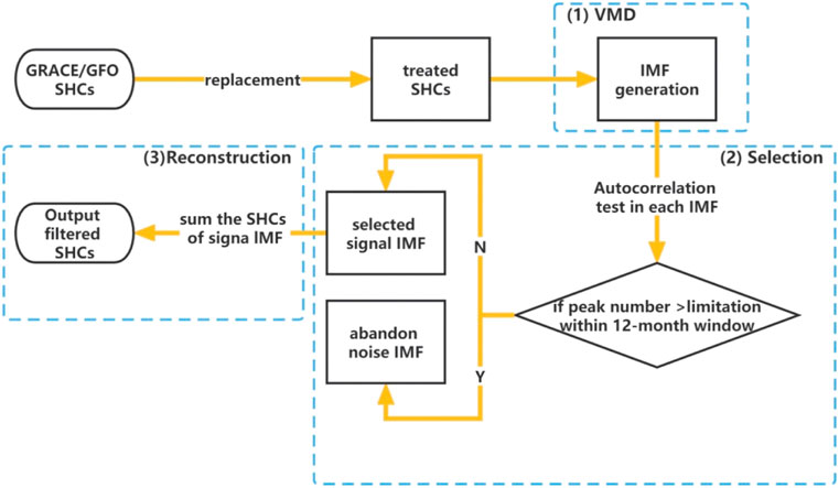
FIGURE 2. The workflow of the TVMD filter for filtering the GRACE/GFO SHCs.

The TEMD filter is similar to the algorithm of the TVMD filter, which is only different in the generation of IMF (i.e., step 1), which is implemented by the EMD approach.

3.5 The SNR index and the three-cornered hat method

Aiming to assess the GRACE/GFO mass field, the SNR index is utilized. Taking into account that measurement errors are approximately equal over land and ocean (i.e., LandError≈OceanError), Chen et al. (2006) developed the SNR index, which is defined as the land-ocean Root Mean Square (RMS) ratio:

$\mathrm{S}\mathrm{N}\mathrm{R}=\frac{\mathrm{R}\mathrm{M}\mathrm{S}\left(Landmass+\mathrm{L}\mathrm{a}\mathrm{n}\mathrm{d}\mathrm{E}\mathrm{r}\mathrm{r}\mathrm{o}\mathrm{r}\right)}{\mathrm{R}\mathrm{M}\mathrm{S}\left(\mathrm{O}\mathrm{c}\mathrm{e}\mathrm{a}\mathrm{n}\mathrm{m}\mathrm{a}\mathrm{s}\mathrm{s}+\mathrm{O}\mathrm{c}\mathrm{e}\mathrm{a}\mathrm{n}\mathrm{E}\mathrm{r}\mathrm{r}\mathrm{o}\mathrm{r}\right)}(8)$

where Landmass/Oceanmass is the true mass field over land/ocean (Chen et al., 2006). To reduce land signal leakage when calculating the RMS over global lands, a 300 km buffer zone is implemented.

The three-cornered hat method provides an alternate assessment to solve the measurement issue of uncertainty when the true signal is absent (Ferreira et al., 2016; Chen J. et al., 2021). In this study, we use this technique to assess the accuracy of our estimates. The detail of this technique is shown in the rich work of Ferreira et al. (2016).

4 Results and discussion

4.1 The spatial results

First, an average GSM product from January 2003 (random selection) is utilized to investigate our filter. The original mass field is contaminated by north-south stripe noise (Figure 3A). After applying the TVMD filter, the TEMD filter, or the P4M6 method, the north-south stripe noise is relieved and the filtered mass field is made up of physical signals plus random and residual stripe noises. In the P4M6 result (Figure 3B), there is still significant stripe noise in low latitudes because of its inadequate process beyond degree 50. For the TEMD and TVMD results, the residual north-south stripe patterns are distributed relatively evenly (Figures 3C, D). But the latter removes more stripe patterns, which must be the noise because the difference between the two results exhibits a stripe pattern rather than the geophysical signals (Figure 3F). Afterward, in comparison to the CSR mascon product (Figure 3E), we find that there is an evident distortion over Greenland in the P4M6 result rather than in the TVMD and TEMD results. Note that this mascon product is truncated up to degree 60 to separate the contribution of signal leakage.

FIGURE 3

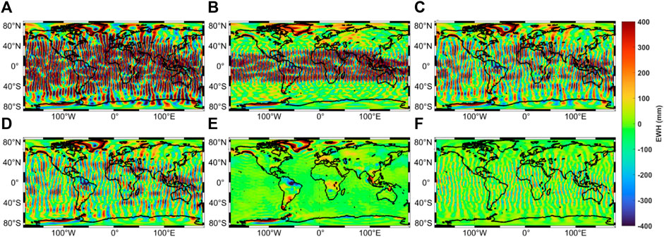
FIGURE 3. The global mass field in January 2003. (A) Without filtering. (B) With the P4M6 method. (C) With the TEMD filter. (D) With the TVMD filter. (E) The CSR mascon product is truncated up to degree 60. (F) The difference between C and D (i.e., C$-$D). Please note that no additional Gaussian filter is adopted.

In addition, our objective is to determine the spatial contribution of extracted patterns in each band (e.g., ${\mathrm{n}}_{\mathrm{s}\mathrm{t}\mathrm{a}\mathrm{r}\mathrm{t}}$ =0 to ${\mathrm{n}}_{\mathrm{e}\mathrm{n}\mathrm{d}}$ =40 in Eq. 1, Figure 4A). In the band ranging from degrees 0 to 50, some minor variations can be observed in the extracted patterns between the two temporal filters and the P4M6 method. But in comparison, beyond degree 50, the P4M6 result exhibits weak filtering due to a lack of adequate processing (Figure 4C). Consequently, this approach retains more stripe noise in the low latitudes. Relatively, the two temporal filters perform sufficient processing beyond degree 50.

FIGURE 4

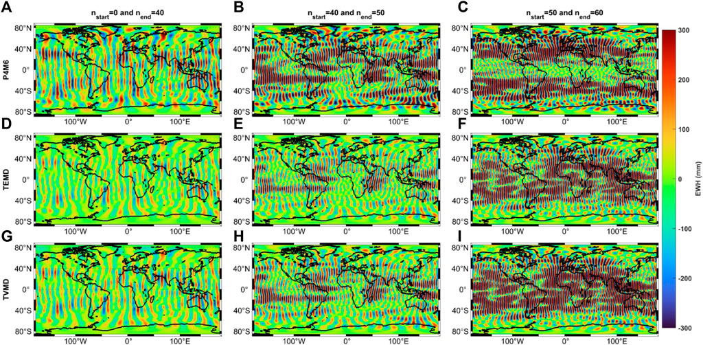
FIGURE 4. The extracted stripe pattern (i.e., the difference between the original and filtered mass field) in each band. (A–C) With the P4M6 method. (D–F) With the TEMD filter. (G–I) With the TVMD filter. (Left) ${\mathrm{n}}_{\mathit{s}\mathit{t}\mathit{a}\mathit{r}\mathit{t}}=0$ and ${\mathrm{n}}_{\mathit{e}\mathit{n}\mathit{d}}=40$. (Middle) ${\mathrm{n}}_{\mathit{s}\mathit{t}\mathit{a}\mathit{r}\mathit{t}}=40$ and ${\mathrm{n}}_{\mathit{e}\mathit{n}\mathit{d}}=50$. (Right) ${\mathrm{n}}_{\mathit{s}\mathit{t}\mathit{a}\mathit{r}\mathit{t}}=50$ and ${\mathrm{n}}_{\mathit{e}\mathit{n}\mathit{d}}=60$.

4.2 The spectral results

While we have already discussed the filtered results in the spatial domain, examining these results in the spectral domain can provide further insight into the differences between the three methods. Figure 5A–E display the amplitude of each SHC. In addition, we compute the differences in magnitude orders between the original and filtered SHCs (Figures 5F–H), which reflect the relative intensity of filtering for each method.

FIGURE 5

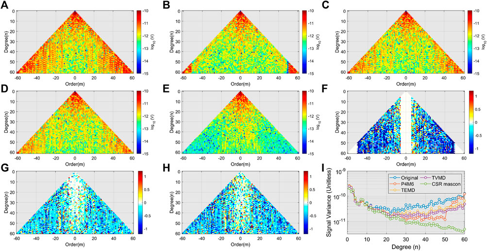
FIGURE 5. The amplitude per SHC. (A) Without filtering. (B–D) After using the P4M6 method, the TEMD filter, and the TVMD filter, respectively. (E) SHCs from the CSR mascon product. (F–H) The difference in B, C, and D concerning A, respectively. Notice (F–H) are the differences in logarithm values, which represent differences in orders of magnitude. (I) The signal variance per degree of each mass field.

The original SHCs and signal variance exhibit unrealistic high amplitudes in higher degrees (Figure 5A, I), which is the major source of the stripe noise. The three methods are effective in reducing the amplitude after degree 20. However, for the P4M6 method, there is a rapid increase after degree 50 because of inadequate filtering in the P4M6 method (Figure 5F). This raise also exists in the TEMD and TVMD signal variance but slower. Compared to other filters, the TVMD filter shows a lower signal variance, which is closer to the CSR mascon product. It adds credibility to our filter.

Additionally, the temporal changes in a part of SHCs are checked (Figure 6). For instance, the P4M6 result exhibits a smaller annual amplitude in $C_{\mathrm{10,10}}$ and significant loss in the long-term signal of $C_{\mathrm{40,10}}$. The P4M6 method may misidentify real geophysical signals and errors in the original SHCs. Conversely, the TVMD and TEMD results preserve more temporal information, which is consistent with the CSR mascon product. It shows the excellent property of our filter in signal reservation in a way.

FIGURE 6

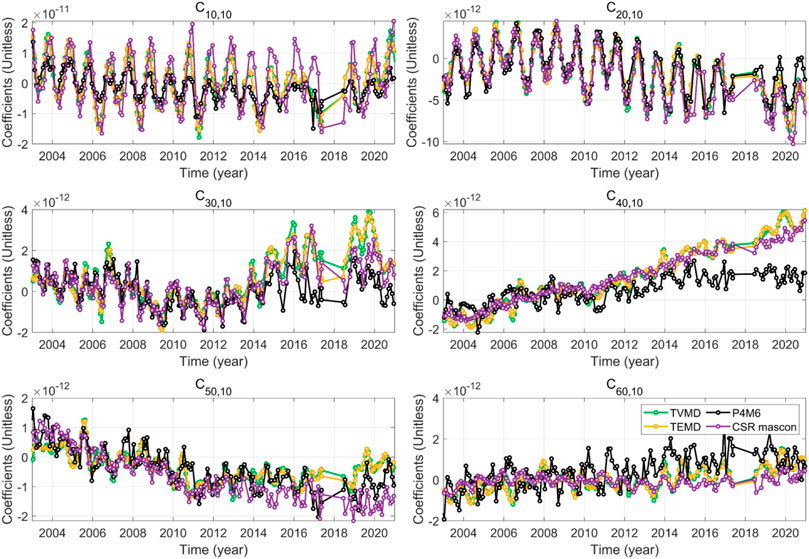
FIGURE 6. The temporal changes in ${\mathit{C}}_{\mathit{10,10}}$, ${\mathit{C}}_{\mathit{20,10}}$, ${\mathit{C}}_{\mathit{30,10}}$, ${\mathit{C}}_{\mathit{40,10}}$, ${\mathit{C}}_{\mathit{50,10}}$, and ${\mathit{C}}_{\mathit{60,10}}$.

4.3 The temporal results

After investigating the spatial and spectral results, we investigate the mass changes in the temporal domain. The basin terrestrial water storage (TWS) changes in Madagascar, Panama, Amazon Basin, and the Caspian Sea are selected for comparison (Figure 7). We compute the filtered TWS changes by the three methods. In addition, the two mascon products from JPL and CSR are also implemented, which are truncated up to degree 60 to separate the contribution of signal leakage. It should be noted that an additional Gaussian filter is not utilized in this comparison.

FIGURE 7

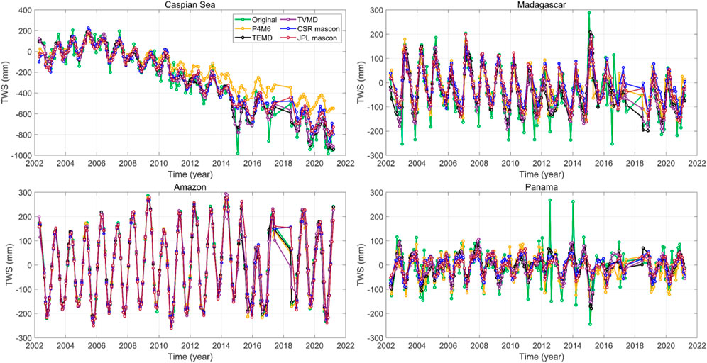
FIGURE 7. The basin TWS changes in the Caspian Sea, Madagascar, Amazon basin, and Panama with four strategies (the original, the TVMD filter, the TEMD filter, and the P4M6 method) and the two mascon products (JPL and CSR). Both mascon products are truncated up to degree 60 to separate the contribution of signal leakage.

The original TWS changes are accompanied by irrational abrupt values, especially in a small-scale basin in low latitudes (e.g., Panama). In comparison to the original result, three methods reduce the unreal variations in the TWS changes. However, the P4M6 method results in a significant loss in long-term signals of the Caspian Sea, which are systematic errors and impossible to be stripe noise. Conversely, the temporal filter can reserve more real long-term signals while suppressing unreal noise. Compared with the other two methods in Panama, the TVMD results are close to the two mascon products. The RMS difference between Panama results obtained from TVMD and those obtained from CSR and JPL are 33.7 and 34.98 mm (Table 1), respectively. This difference is approximately 0.7 mm smaller than that derived from TEMD.

TABLE 1

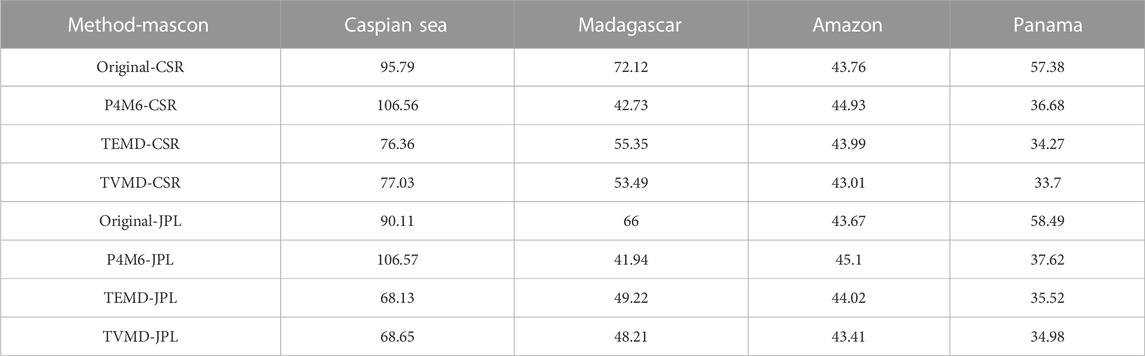
TABLE 1. The RMS (Unit: mm) of the difference in the TWS changes between the filtered result and the two mascon products that truncated up to degree 60.

4.4 Assessment of the TVMD filter

The various investigations mentioned above provide support for the reliability of the TVMD filter. To quantify the improvement achieved by the TVMD filter, the original and filtered mass fields are assessed by two metrics (Figure 8): 1) the SNR index and 2) the regional Standard Deviation (STD) in Panama. The former is the average SNR for all available months. The latter is the latitudinal cosine weighted average of the gridded STD in Panama, which is provided by the three-cornered hat method. For both metrics, the TVMD filter outperforms the P4M6 method and the TEMD filter. After applying the TVMD filter, the SNR index increases from 1.68 to 2.14, and the STD improves from 121 mm to 70 mm, highlighting the effectiveness of our filter in improving the accuracy of mass changes in Panama.

FIGURE 8

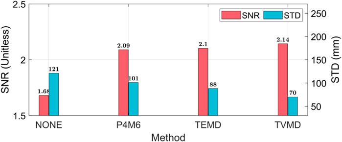
FIGURE 8. The regional average STD in Panama and the SNR. Please note that no additional Gaussian filter is adopted.

4.5 Validation of the improved mass changes

The two metrics show that the TVMD filter improves the SNR and reduces the uncertainty in Panama. Afterward, an additional 300 km Gaussian filter is used to further reduce residual noise in the mass field after using the three methods. The forward modeling technique is utilized to restore the leakage signal in the mass field of each available month by iteration (Chen et al., 2015). In the forward modeling technique, the model undergoes iterative updates until the difference between the filtered model and the filtered observation is minimized below a specified threshold (Doumbia et al., 2020; Zhou et al., 2022). The final TWS changes with three methods and the two mascon products are shown in Figure 9.

FIGURE 9

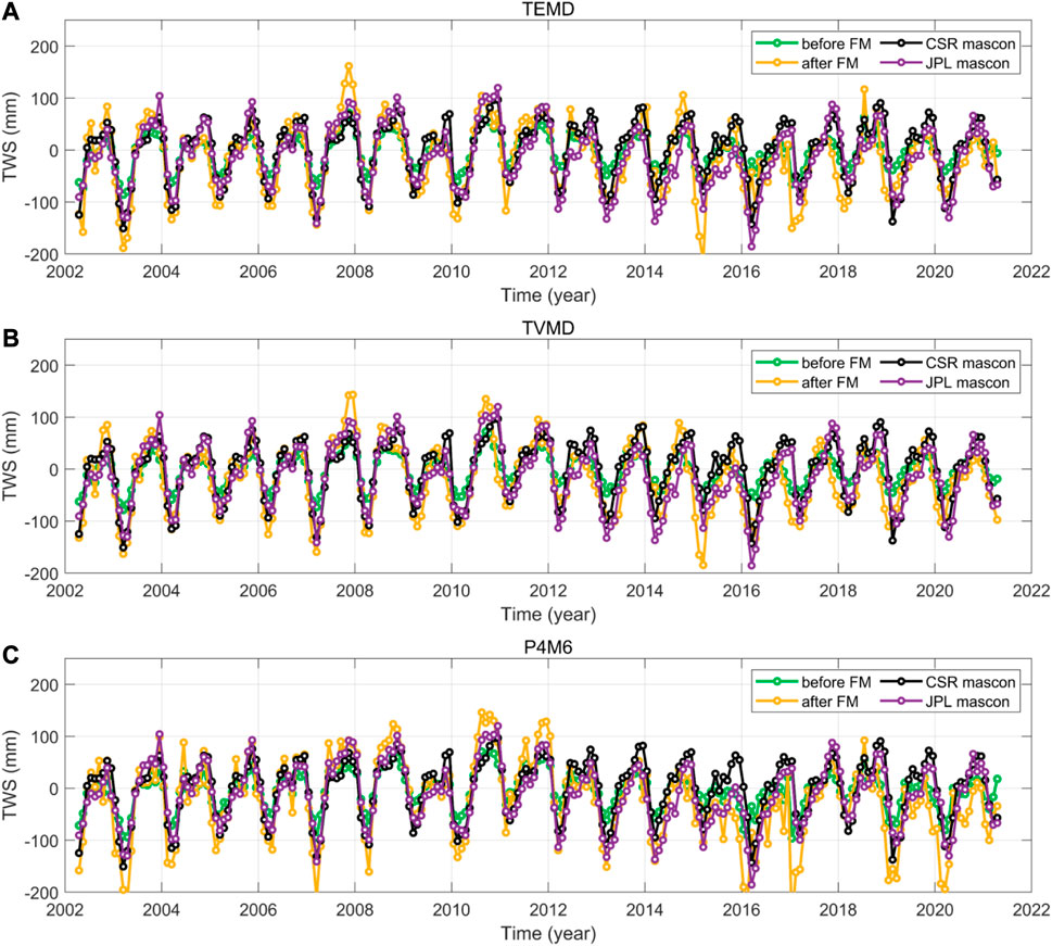
FIGURE 9. The basin TWS changes in Panama after and before using the forward modeling (FM) technique. (A) With the TEMD filter. (B) With the TVMD filter. (C) With the P4M6 method. The two mascon products from CSR and JPL are implemented without truncation in this comparison. The missing value of the time series is interpolated by the iterative singular spectrum analysis.

After using the forward modeling technique, the annual amplitude of the three methods is close to the two mascon products. The P4M6 and TEMD results exhibit more suspected abrupt changes that might be noise, which must be sourced from the noise accumulation in iteration. In contrast, the TVMD results are more stable and are close to both mascon products. Among the three methods, our filter exhibits the minimum difference concerning the two mascon products in the TWS changes (Table 2). The RMS of the difference from CSR and JPL mascon is 44.45 and 42.3 mm, respectively.

TABLE 2

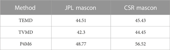
TABLE 2. The RMS (Unit: mm) of the difference in the basin TWS changes between the two mascon products and the final filtered result.

Afterward, comparison with the in situ groundwater observation (GW1 and GW2) can further increase the confidence of our results. According to the water balance equation (Chen et al., 2016), we compute the basin GWS in Panama by subtracting soil moisture storage change from the TWS changes (Figure 10). All five GWS changes have poor correlations with the GW2 observation, possibly due to the poor observational quality. What’s more, the TVMD result achieves the highest correlation of 0.72 with the GW1 observation (Table 3). This comparison indirectly verifies the reliability of our method, and it indicated that our result seems to be sensitive to small-scale mass signals that cannot be detected in the mascon product.

FIGURE 10

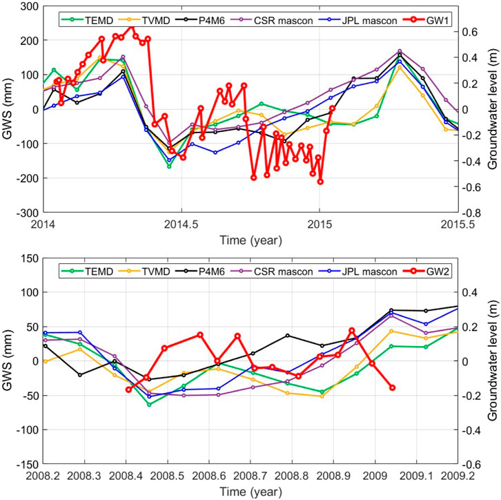
FIGURE 10. The basin GWS changes and the in situ groundwater observations GW1 (Top) and GW2 (Down). The GWS changes are derived from the above final-filtered TWS changes of three methods and the two mascon products subtracting the soil moisture storage.

TABLE 3

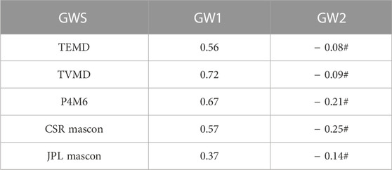
TABLE 3. The Pearson correlation coefficient between the five GWS changes and the two groundwater observations. The correlation value with # denotes the significant value p >0.05.

5 Conclusion

In this study, our focus is on estimating the mass change in Panama using GRACE SHCs solutions, which are affected by stripe noise. To address the limitations, we propose the TVMD filter. Our approach considers applying the VMD algorithm to filter the time series of each SHC individually.

To evaluate the effectiveness of our method, we compare the results with the reliable mascon product. The comparison is carried out in terms of spatial, spectral, and temporal domains. It can be concluded that: 1) The filtering intensity of our filter distributes evenly in the spatial domain. 2) Compared with the P4M6 method, the TEMD and TVMD filter mainly reduces the signal variance after degree 50, and the TVMD signal variance per degree is smaller than that of the TEMD. It explains the source of the improvement of our filter. 3) Compared with the P4M6 method, the temporal filter can preserve the temporal property of the mass field.

We also use the SNR index and the three-cornered hat method for assessment. Our filtering technique outperforms the previous two methods, achieving the highest SNR (2.14) and the lowest uncertainty (70 mm) in Panama for all available months.

Afterward, the two mascon products and the short-term groundwater observations are implemented to assess our estimates of the TWS changes in Panama. Our results have the closest agreement with the mascon products. The RMS difference in the final TWS changes between our results and the two mascon products (JPL and CSR) is 42.3 mm and 44.45 mm, respectively, and we observe the highest correlation coefficient (0.72) between our estimate of basin GWS and the in situ groundwater observations. This suggests that our method seems to be effective in detecting small-scale signals compared to the mascon products.

In this study, we have established that SHC products have the potential to uncover the mass change in Panama. However, the inversion and verification of these mass changes remain challenging. Overall, our work provides valuable insights into examining the TWS and GWS changes in small-scale basins located in low latitudes. It also serves as a reference for future research in this field.

Data availability statement

The original contributions presented in the study are included in the article/supplementary material, further inquiries can be directed to the corresponding author.

Author contributions

GJ performed the data processing, analyzed the results, and drafted the manuscript. CX designed and conducted this study and revised the manuscript. CY checked the performance of the new filter and revised the manuscript. All authors contributed to the article and approved the submitted version.

Funding

This research was funded by the National Natural Science Foundation of China (Grant no. 41974014 and 42274004) and the Natural Science Foundation of Guangdong Province, China (Grant Nos. 2022A1515010396).

Acknowledgments

We appreciate the constructive and rich comments from the editor and two reviewers, which led to an excellent improvement of the manuscript.

Conflict of interest

The authors declare that the research was conducted in the absence of any commercial or financial relationships that could be construed as a potential conflict of interest.

Publisher’s note

All claims expressed in this article are solely those of the authors and do not necessarily represent those of their affiliated organizations, or those of the publisher, the editors and the reviewers. Any product that may be evaluated in this article, or claim that may be made by its manufacturer, is not guaranteed or endorsed by the publisher.

References

Beck, H. E., Zimmermann, N. E., McVicar, T. R., Vergopolan, N., Berg, A., and Wood, E. F. (2018). Present and future Koppen-Geiger climate classification maps at 1-km resolution. Sci. Data 5, 180214. doi:10.1038/sdata.2018.214

PubMed Abstract | CrossRef Full Text | Google Scholar

Chambers, D. P., and Bonin, J. A. (2012). Evaluation of Release-05 GRACE time-variable gravity coefficients over the ocean. Ocean Sci. 8 (5), 859–868. doi:10.5194/os-8-859-2012

CrossRef Full Text | Google Scholar

Chen, J., Famiglietti, J. S., Scanlon, B. R., and Rodell, M. (2016). Erratum to: groundwater storage changes: present status from GRACE observations. Surv. Geophys. 37 (3), 701. doi:10.1007/s10712-016-9370-6

CrossRef Full Text | Google Scholar

Chen, J. L., Wilson, C. R., Li, J., and Zhang, Z. Z. (2015). Reducing leakage error in GRACE-observed long-term ice mass change: a case study in west Antarctica. J. Geodesy 89 (9), 925–940. doi:10.1007/s00190-015-0824-2

CrossRef Full Text | Google Scholar

Chen, J. L., Wilson, C. R., and Seo, K. W. (2006). Optimized smoothing of gravity recovery and climate experiment (GRACE) time-variable gravity observations. J. Geophys. Research-Solid Earth 111 (B6), 11. doi:10.1029/2005jb004064

CrossRef Full Text | Google Scholar

Chen, J. L., Wilson, C. R., Tapley, B. D., Blankenship, D., and Young, D. (2008). Antarctic regional ice loss rates from GRACE. Earth Planet. Sci. Lett. 266 (1-2), 140–148. doi:10.1016/j.epsl.2007.10.057

CrossRef Full Text | Google Scholar

Chen, J. L., Wilson, C. R., Tapley, B. D., Save, H., and Cretaux, J. F. (2017). Long-term and seasonal Caspian Sea level change from satellite gravity and altimeter measurements. J. Geophys. Research-Solid Earth 122 (3), 2274–2290. doi:10.1002/2016JB013595

CrossRef Full Text | Google Scholar

Chen, J., Tapley, B., Tamisiea, M. E., Save, H., Wilson, C., Bettadpur, S., et al. (2021a). Microphysical modeling of carbonate fault friction at slip rates spanning the full seismic cycle. J. Geophys. Research-Solid Earth 126 (9), e2020JB021024. doi:10.1029/2020JB021024

CrossRef Full Text | Google Scholar

Chen, Q., Shen, Y., Kusche, J., Chen, W., Chen, T., and Zhang, X. (2021b). High-Resolution GRACE monthly spherical harmonic solutions. J. Geophys. Research-Solid Earth 126 (1). doi:10.1029/2019jb018892

CrossRef Full Text | Google Scholar

Cheng, M., Tapley, B. D., and Ries, J. C. (2013). Deceleration in the Earth's oblateness. J. Geophys. Research-Solid Earth 118 (2), 740–747. doi:10.1002/jgrb.50058

CrossRef Full Text | Google Scholar

Crossley, D., Hinderer, J., Boy, J. P., and Pierce, D. W. (2005). Time variation of the European gravity field from superconducting gravimeters. Geophys. J. Int. 161 (2), 257–264. doi:10.1111/j.1365-246X.2005.02586.x

CrossRef Full Text | Google Scholar

Doumbia, C., Castellazzi, P., Rousseau, A. N., and Amaya, M. (2020). High resolution mapping of ice mass loss in the gulf of Alaska from constrained forward modeling of GRACE data. Front. Earth Sci. 7. doi:10.3389/feart.2019.00360

CrossRef Full Text | Google Scholar

Dragomiretskiy, K., and Zosso, D. (2014). Variational mode decomposition. Ieee Trans. Signal Process. 62 (3), 531–544. doi:10.1109/tsp.2013.2288675

CrossRef Full Text | Google Scholar

Duan, X. J., Guo, J. Y., Shum, C. K., and van der Wal, W. (2009). On the postprocessing removal of correlated errors in GRACE temporal gravity field solutions. J. Geodesy 83 (11), 1095–1106. doi:10.1007/s00190-009-0327-0

CrossRef Full Text | Google Scholar

Feng, Z.-k., Niu, W.-j., Tang, Z.-y., Jiang, Z.-q., Xu, Y., Liu, Y., et al. (2020). Monthly runoff time series prediction by variational mode decomposition and support vector machine based on quantum-behaved particle swarm optimization. J. Hydrology 583, 124627. doi:10.1016/j.jhydrol.2020.124627

CrossRef Full Text | Google Scholar

Ferreira, V. G., Montecino, H. D. C., Yakubu, C. I., and Heck, B. (2016). Uncertainties of the Gravity Recovery and Climate Experiment time-variable gravity-field solutions based on three-cornered hat method. J. Appl. Remote Sens. 10, 015015. doi:10.1117/1.Jrs.10.015015

CrossRef Full Text | Google Scholar

Ferreira, V., Yong, B., Montecino, H., Ndehedehe, C. E., Seitz, K., Kutterer, H., et al. (2023). Estimating GRACE terrestrial water storage anomaly using an improved point mass solution. Sci. Data 10 (1), 234. doi:10.1038/s41597-023-02122-1

PubMed Abstract | CrossRef Full Text | Google Scholar

Gonzalez-Valoys, A. C., Vargas-Lombardo, M., Jimenez-Ballesta, R., Arrocha, J., Gutierrez, E., Garcia-Ordiales, E., et al. (2022). Characterization of the soil and rock hosting an aquifer with possible uses for drinking water and irrigation in SE Panama City using Geotechnical, Geophysical and Geochemical parameters. Environ. Earth Sci. 81 (10), 283. doi:10.1007/s12665-022-10412-x

CrossRef Full Text | Google Scholar

Han, S. C., Shum, C. K., Jekeli, C., Kuo, C. Y., Wilson, C., and Seo, K. W. (2005). Non-isotropic filtering of GRACE temporal gravity for geophysical signal enhancement. Geophys. J. Int. 163 (1), 18–25. doi:10.1111/j.1365-246X.2005.02756.x

CrossRef Full Text | Google Scholar

Huan, C. M., Wang, F. W., and Zhou, S. J. (2022). Empirical mode decomposition for post-processing the GRACE monthly gravity field models. Acta Geodyn. Geomaterialia 19 (4), 281–290. doi:10.13168/agg.2022.0013

CrossRef Full Text | Google Scholar

Huang, N. E., Shen, Z., Long, S. R., Wu, M. L. C., Shih, H. H., Zheng, Q. N., et al. (1998). The empirical mode decomposition and the Hilbert spectrum for nonlinear and non-stationary time series analysis. Proc. R. Soc. a-Mathematical Phys. Eng. Sci. 454 (1971), 903–995. doi:10.1098/rspa.1998.0193

CrossRef Full Text | Google Scholar

King, M. A., and Padman, L. (2005). Accuracy assessment of ocean tide models around Antarctica. Geophys. Res. Lett. 32 (23), L23608. doi:10.1029/2005gl023901

CrossRef Full Text | Google Scholar

Klees, R., Liu, X., Wittwer, T., Gunter, B. C., Revtova, E. A., Tenzer, R., et al. (2008a). A comparison of global and regional GRACE models for land hydrology. Surv. Geophys. 29 (4-5), 335–359. doi:10.1007/s10712-008-9049-8

CrossRef Full Text | Google Scholar

Klees, R., Revtova, E. A., Gunter, B. C., Ditmar, P., Oudman, E., Winsemius, H. C., et al. (2008b). The design of an optimal filter for monthly GRACE gravity models. Geophys. J. Int. 175 (2), 417–432. doi:10.1111/j.1365-246X.2008.03922.x

CrossRef Full Text | Google Scholar

Li, J., Chen, J., Li, Z., Wang, S.-Y., and Hu, X. (2017). Ellipsoidal correction in GRACE surface mass change estimation. J. Geophys. Research-Solid Earth 122 (11), 9437–9460. doi:10.1002/2017jb014033

CrossRef Full Text | Google Scholar

Loomis, B. D., Rachlin, K. E., Wiese, D. N., Landerer, F. W., and Luthcke, S. B. (2020). Replacing GRACE/GRACE-FO with satellite laser ranging: impacts on antarctic ice sheet mass change. Geophys. Res. Lett. 47 (3). doi:10.1029/2019gl085488

CrossRef Full Text | Google Scholar

Nerem, R. S., Wahr, J. M., and Leuliette, E. W. (2003). Measuring the distribution of ocean mass using GRACE. Space Sci. Rev. 108 (1-2), 331–344. doi:10.1023/a:1026275310832

CrossRef Full Text | Google Scholar

Peltier, W. R., Argus, D. F., and Drummond, R. (2018). Comment on "An Assessment of the ICE-6G_C (VM5a) Glacial Isostatic Adjustment Model" by Purcell et al. J. Geophys. Research-Solid Earth 123 (2), 2019–2028. doi:10.1002/2016JB013844

CrossRef Full Text | Google Scholar

Pu, L., Fan, D., You, W., Yang, X., Nigatu, Z. M., and Jiang, Z. (2022). Extracting terrestrial water storage signals from GRACE solutions in the Amazon Basin using an iterative filtering approach. Remote Sens. Lett. 13 (1), 14–23. doi:10.1080/2150704x.2021.1981557

CrossRef Full Text | Google Scholar

Rangelova, E., van der Wal, W., Braun, A., Sideris, M. G., and Wu, P. (2007). Analysis of Gravity Recovery and Climate Experiment time-variable mass redistribution signals over North America by means of principal component analysis. J. Geophys. Research-Earth Surf. 112 (F3), F03002. doi:10.1029/2006jf000615

CrossRef Full Text | Google Scholar

Ray, R. D., and Ponte, R. M. (2003). Barometric tides from ECMWF operational analyses. Ann. Geophys. 21 (8), 1897–1910. doi:10.5194/angeo-21-1897-2003

CrossRef Full Text | Google Scholar

Rodell, M., Houser, P., Jambor, U., Gottschalck, J., Mitchell, K., Meng, C.-J., et al. (2004). The global land data assimilation system. Bull. Am. Meteorological Soc. 85 (3), 381–394. doi:10.1175/BAMS-85-3-381

CrossRef Full Text | Google Scholar

Sasgen, I., Martinec, Z., and Fleming, K. (2006). Wiener optimal filtering of GRACE data. Studia Geophys. Geod. 50 (4), 499–508. doi:10.1007/s11200-006-0031-y

CrossRef Full Text | Google Scholar

Save, H., Bettadpur, S., and Tapley, B. D. (2016). High-resolution CSR GRACE RL05 mascons. J. Geophys. Research-Solid Earth 121 (10), 7547–7569. doi:10.1002/2016jb013007

CrossRef Full Text | Google Scholar

Shen, Y., Wang, F., and Chen, Q. (2021). Weighted multichannel singular spectrum analysis for post-processing GRACE monthly gravity field models by considering the formal errors. Geophys. J. Int. 226 (3), 1997–2010. doi:10.1093/gji/ggab199

CrossRef Full Text | Google Scholar

Sprenger, M., Oelmann, Y., Weihermuller, L., Wolf, S., Wilcke, W., and Potvin, C. (2013). Tree species and diversity effects on soil water seepage in a tropical plantation. For. Ecol. Manag. 309, 76–86. doi:10.1016/j.foreco.2013.03.022

CrossRef Full Text | Google Scholar

Swenson, S., Chambers, D., and Wahr, J. (2008). Estimating geocenter variations from a combination of GRACE and ocean model output. J. Geophys. Research-Solid Earth 113 (B8), B08410. doi:10.1029/2007jb005338

CrossRef Full Text | Google Scholar

Swenson, S., and Wahr, J. (2002). Methods for inferring regional surface-mass anomalies from Gravity Recovery and Climate Experiment (GRACE) measurements of time-variable gravity. J. Geophys. Research-Solid Earth 107 (B9), ETG 3-1–ETG 3-13. doi:10.1029/2001jb000576

CrossRef Full Text | Google Scholar

Swenson, S., Wahr, J., and Milly, P. C. D. (2003). Estimated accuracies of regional water storage variations inferred from the Gravity Recovery and Climate Experiment (GRACE). Water Resour. Res. 39 (8). doi:10.1029/2002wr001808

CrossRef Full Text | Google Scholar

Swenson, S., and Wahr, J. (2006). Post-processing removal of correlated errors in GRACE data. Geophys. Res. Lett. 33 (8), L08402. doi:10.1029/2005gl025285

CrossRef Full Text | Google Scholar

Syed, T. H., Famiglietti, J. S., Rodell, M., Chen, J., and Wilson, C. R. (2008). Analysis of terrestrial water storage changes from GRACE and GLDAS. Water Resour. Res. 44 (2). doi:10.1029/2006wr005779

CrossRef Full Text | Google Scholar

Wahr, J., Molenaar, M., and Bryan, F. (1998). Time variability of the Earth's gravity field: hydrological and oceanic effects and their possible detection using GRACE. J. Geophys. Research: solid Earth 103 (B12), 30205–30229. doi:10.1029/98JB02844

CrossRef Full Text | Google Scholar

Wang, L., Davis, J. L., Hill, E. M., and Tamisiea, M. E. (2016). Stochastic filtering for determining gravity variations for decade-long time series of GRACE gravity. J. Geophys. Research-Solid Earth 121 (4), 2915–2931. doi:10.1002/2015jb012650

CrossRef Full Text | Google Scholar

Wiese, D. N., Landerer, F. W., and Watkins, M. M. (2016). Quantifying and reducing leakage errors in the JPL RL05M GRACE mascon solution. Water Resour. Res. 52 (9), 7490–7502. doi:10.1002/2016wr019344

CrossRef Full Text | Google Scholar

Yi, S., and Sneeuw, N. (2021). Filling the data gaps within GRACE missions using singular spectrum analysis. J. Geophys. Research-Solid Earth 126 (5). doi:10.1029/2020jb021227

CrossRef Full Text | Google Scholar

Zaitchik, B. F., Rodell, M., and Reichle, R. H. (2008). Assimilation of GRACE terrestrial water storage data into a land surface model: results for the Mississippi river basin. J. Hydrometeorol. 9 (3), 535–548. doi:10.1175/2007jhm951.1

CrossRef Full Text | Google Scholar

Zhang, Z. Z., Chao, B. F., Lu, Y., and Hsu, H. T. (2009). An effective filtering for GRACE time-variable gravity: fan filter. Geophys. Res. Lett. 36, L17311. doi:10.1029/2009gl039459

CrossRef Full Text | Google Scholar

Zhou, H., Dai, M., Wang, P., Wei, M., Tang, L., Xu, S., et al. (2022). Assessment of GRACE/GRACE follow-on terrestrial water storage estimates using an improved forward modeling method: a case study in africa. Front. Earth Sci. 9. doi:10.3389/feart.2021.796723

CrossRef Full Text | Google Scholar