Sensitivity of the second seismic moments resolution to determine the fault parameters of moderate earthquakes

Second-degree seismic moments provide a simple description of the spatiotemporal extent of the earthquake source. Finite source attributes such as rupture length, width, duration, velocity, and propagation direction can be estimated by computing second-degree seismic moments without the need for a predefined rupture model. This is achieved by analyzing the properties of apparent source time functions (ASTFs) obtained from seismic signals recorded at different stations after eliminating instrument responses and path effects. In this study, to define the limits of its application in the analysis of small earthquakes and to evaluate the sensitivity and reliability of the results to uncertainties due to observations and prior knowledge, we modeled a synthetic seismic source and examined how potential uncertainties in hypocentral depth, velocity model, focal mechanism, source duration, and number of recording stations can affect the inversion results. An accurate ASTF is essential to obtain robust results and our findings show that the mean values of the key source parameters, i.e., fracture size, source duration, and rupture velocity, are generally well reproduced in all sensitivity tests, with some exceptions, within the standard deviation. We also demonstrate that large uncertainties in the hypocentral depth and inaccurate velocity models introduce a significant bias, especially in rupture size and average centroid velocity, indicating the strong influence of ray path calculation in the inversion process. These resolution limits must therefore be taken into account when interpreting the results obtained with this technique.

1 Introduction

Earthquake source parameters such as rupture size, duration, velocity, and propagation, help us understand earthquake physics, fault zone properties, and rupture dynamics conditions, which have significant implications for seismic hazard assessment. Effects due to source finiteness, such as directivity, are usually associated with high-magnitude earthquakes (Ammon et al., 1993; Somerville et al., 1996), but they can also enable moderate earthquakes to cause severe unexpected damage. For example, the directivity effect can lead to potentially destructive pulses at low frequencies characterized by large amplitudes of ground motion (Boatwright, 2007; Kurzon et al., 2014; Moratto et al., 2017; Ertuncay and Costa, 2021; Ertuncay et al., 2021). Therefore, knowledge of the kinematic finite source parameters and expected rupture directions for high and moderate magnitude events is critical for earthquake engineering applications (Moratto et al., 2021; Somala et al., 2021; Moratto et al., 2023) and for appropriate risk assessment.

Estimation of source parameters for high magnitude earthquakes is usually feasible. However, the accurate determination of these parameters for moderate and small earthquakes remains a major challenge. Namely, while far-field records and geodetic data can provide complementary information for large earthquakes, geodetic data are lacking for small to medium events, and only seismic records from nearby stations are available. As a result, the kinematic properties of small earthquakes are often difficult to determine, and simple models are often used to represent these events (e.g., McGuire, 2004; Shearer et al., 2006; Convertito et al., 2013; Calderoni et al., 2015; Abercrombie et al., 2017; Moratto et al., 2019; Colavitti et al., 2022; Yoshida et al., 2022) although improved records show that source complexity is also common for small earthquake ruptures (e.g., Calderoni and Abercrombie, 2023 and reference therein).

A critical task in determining finite source attributes for moderate and low magnitude earthquakes requires good removal of path and site effects. For large earthquakes, this is usually done by synthesizing Green’s functions with a suitable velocity model to fit the low-frequency component (less than 5 Hz) of the observed waveforms (e.g., Ji et al., 2002; Beresnev et al., 2003; Yue et al., 2012; Moratto et al., 2015). For small to moderate earthquakes, the existing velocity structures usually have insufficient resolution and accuracy, leading to reliability problems in the high-frequency range (greater than or equal to 5 Hz). To address this problem, a number of methods based on empirical Green’s function (EGF) deconvolution have been developed in recent decades (e.g., Hartzell, 1978; Mueller, 1985; Mori, 1993; Ammon et al., 1993; Hough, 1997; Lanza et al., 1999; McGuire, 2004; de Lorenzo et al., 2008; Meng et al., 2020). EGF methods use a collocated earthquake with magnitudes typically 1.5–2.5 units smaller than the target event with a similar focal mechanism to account for path effects. The deconvolution process of the target event by an EGF automatically removes path and site effects without the need for a velocity model to synthesize Green’s functions. Although the EGF offers several advantages, its use presents certain difficulties, and selecting an appropriate EGF can be difficult, even when working with an extensive database (Calderoni and Abercrombie, 2023). Focal mechanisms are often not available for small earthquakes, and numerous studies have shown that even for small earthquakes, the effect of directivity cannot be neglected when selecting an EGF (Abercrombie, 2015; Calderoni et al., 2015; Calderoni et al., 2017).

The simplest general representation of an earthquake that contains information about rupture extension and directivity is the point-source representation plus the variances or second-degree moments of the moment-release distribution (e.g., Silver, 1983; McGuire et al., 2001). The hypocenter and origin time of the earthquake correspond to the spatial and temporal average (first-degree moment) of the release moment distribution. The information on rupture extension, characteristic duration, and direction of rupture propagation correspond to the variance of the moment distribution in the spatial, temporal, and spatiotemporal domains (second-degree moments). Seismic moments are calculated from apparent durations measured from apparent source time functions (ASTF) for each station after removing path effects. The ASTF obtained using EGF deconvolution (McGuire, 2004; 2017), represents the difference between the source time function (STF) of the main earthquake and that of the EGF earthquake from the direction of observation at each station. Thus, the ASTF is the projection of the rupture process onto the seismic ray path, and its properties also depend on azimuth and take-off angles (e.g., McGuire et al., 2001; McGuire, 2004; Stich et al., 2005; Yoshida and Kanamori, 2023). For a unilateral rupture, the ASTF observed by stations in the propagation direction would be significantly shorter than the ASTF of stations in the opposite direction.

A major advantage of the second moments method is that it can be theoretically applied to all earthquakes, regardless of their magnitude and complexity, and without requiring the assumptions of an a priori source model (e.g., McGuire, 2004; Fan and McGuire, 2018; Meng et al., 2020; Meng and Fan, 2021). It is also a consistent tool for evaluating scaling relationships between finite source attributes and earthquake magnitudes for large and small earthquakes (McGuire and Kaneko, 2018) and for resolving fault-plane ambiguity. However, elimination of the path effect is critical, and a biased ASTF calculation would lead to inaccurate calculations of the second seismic moments.

In this study, we consider second-degree seismic moments to provide a simple, model-free description of earthquake rupture and we evaluate, through synthetic tests, the sensitivity of the solutions to uncertainties in key input parameters to investigate the limitations of the method in the study of small earthquakes.

To achieve this goal, we conducted a synthetic test for a magnitude 4.6 earthquake and examined the effects of potential uncertainties in source duration, hypocentral depth, station configuration, focal mechanism, and velocity model, considering unilateral and bilateral rupture scenarios. In view of future analyses to be performed with real data, we located the hypothetical earthquake in central Italy, an area with good station coverage by the Italian seismic network (Amato et al., 2006) and the Italian accelerogram network (Costa et al., 2022). The wealth of data recorded in this very active seismic area makes it an excellent natural laboratory for the study of source characteristics, and there are numerous studies on the subject of sources published after the 1997 Umbria and Marche earthquakes, 2009 L’Aquila, and 2016 Amatrice earthquakes (e.g., Chimera et al., 2003; Bindi et al., 2009; Cultrera et al., 2009; Moratto and Saraò, 2012; Rovelli and Calderoni, 2014; Calderoni et al., 2015; Calderoni et al., 2017; Convertito et al., 2017; Wang et al., 2019).

The following sections describe the method used to determine the source parameters and the synthetic input model, as well as the sensitivity tests performed. Finally, the results and the strengths and weaknesses of the method are discussed, providing valuable insights for applying the approach to real earthquake data.

2 Method

2.1 The second seismic moments

The moment release variations along a fault can be described by the relation

$\dot{M}‗\left(\underset{\_}{r},t\right)=\widehat{M}‗\dot{f}\left(\underset{\_}{r},t\right)(1)$

where $\dot{M}̳$ is the moment rate function which varies in both time and space, $\widehat{M}$ is the seismic moment tensor and $\dot{f}\left(\underset{\_}{r},t\right)$ is a scalar function describing the spatial and temporal distribution of the moment release along the fault (McGuire, 2004; McGuire and Kaneko, 2018; Meng et al., 2020). When $\dot{f}\left(\underset{\_}{r},t\right)$ is integrated over the entire source volume, it represents the normalized STF. The zero degree moment is the standard seismic moment (M₀), while the first degree moments μ^(1,0) and μ^(0,1) represent the centroid location ( ${\underset{\_}{r}}_0$) and time $\left(t_0\right)$ of an earthquake and the spatio-temporal means of its moment release:

$\begin{array}{c}{\underset{\_}{r}}_0={\underset{\_}{\mu }}^{\left(\mathrm{1,0}\right)}=\iint \dot{f}\left(\underset{\_}{r},t\right)\underset{\_}{r}dVdt,\\ t_0={\mu }^{\left(\mathrm{0,1}\right)}=\iint \dot{f}\left(\underset{\_}{r},t\right)tdVdt.\end{array}(2)$

The second seismic moments about a point ( $\underset{\_}{r_0}$) and time $\left(t_0\right)$ represent the second order space and time moments, i.e., the variance, of $\dot{f}\left(\underset{\_}{r},t\right)$, and are defined as follows:

${\widehat{\mu ̳}}^{\left(\mathrm{2,0}\right)}=\iint \dot{f}\left(\underset{\_}{r},t\right){\left({\underset{\_}{r}-\underset{\_}{r}}_0\right)}^T\left({\underset{\_}{r}-\underset{\_}{r}}_0\right)dVdt,$

${\widehat{\mu }}^{\left(\mathrm{0,2}\right)}=\iint \dot{f}\left(\underset{\_}{r},t\right)\left({t-t}_0\right)\left({t-t}_0\right)dVdt,(3)$

${\widehat{\underset{\_}{\mu }}}^{\left(\mathrm{1,1}\right)}=\iint \dot{f}\left(\underset{\_}{r},t\right)\left({\underset{\_}{r}-\underset{\_}{r}}_0\right)\left({t-t}_0\right)dVdt.$

where ${\widehat{\mu ̳}}^{\left(\mathrm{2,0}\right)}$ is the second spatial moment associated with the rupture extent, ${\widehat{\mu }}^{\left(\mathrm{0,2}\right)}$ is the temporal moment, a scalar (one unique element) associated with the rupture duration; and ${\widehat{\underset{\_}{\mu }}}^{\left(\mathrm{1,1}\right)}$ is called mixed moment and it is a column vector (three unique elements) associated with the rupture propagation (McGuire et al., 2001; Meng et al., 2020).

The second moments are related to the characteristic rupture duration ${\tau }_c$,

${\tau }_c=2\sqrt{{\widehat{\mu }}^{\left(\mathrm{0,2}\right)}}(4)$

the characteristic rupture dimension $x_c$, the centroid rupture velocity ${\underset{\_}{v}}_0$, the characteristic velocity $v_c$ as follows (Silver, 1983; McGuire et al., 2001):

$\begin{array}{c}{x}_c\left(\widehat{n}\right)=2\sqrt{{\widehat{n}}^T{\widehat{\mu ̳}}^{\left(\mathrm{2,0}\right)}\widehat{n}},\\ {\underset{\_}{v}}_0=\frac{{\widehat{\underset{\_}{\mu }}}^{\left(\mathrm{1,1}\right)}}{{\widehat{\mu }}^{\left(\mathrm{0,2}\right)}},\\ v_c=\frac{L_c}{{\tau }_c}.\end{array}(5)$

where $\widehat{n}$ indicate the rupture direction. For a planar source, $x_c\left(\widehat{n}\right)$ will be identically zero in the direction normal to the fault plane, providing a test for discriminating between the two candidate nodal planes of an event’s focal mechanism.

The largest eigenvalue of $x_c\left(\widehat{n}\right)$ represents the characteristic rupture length ($L_c$) while the second largest eigenvalue is the characteristic rupture width ($W_c$). An earthquake rupture can be quantified by the directivity ratio, that ranges from 0 for a perfectly symmetric bilateral rupture to 1 for a uniform slip unilateral rupture (McGuire et al., 2001), and is defined as

$dir=\frac{\left.{\left|\underset{\_}{v}\right.}_0\right|}{v_c}(6)$

The second moments are related to the azimuthal variations in the duration of ASTFs at a given station as

${\widehat{\mu }}^{\left(\mathrm{0,2}\right)}\left(\underset{\_}{s}\right)={\widehat{\mu }}^{\left(\mathrm{0,2}\right)}-2\left(\underset{\_}{s}\right)\cdot {\widehat{\underset{\_}{\mu }}}^{\left(\mathrm{1,1}\right)}+\underset{\_}{s}\cdot {\widehat{\mu ̳}}^{\left(\mathrm{2,0}\right)}\cdot \underset{\_}{s}(7)$

where ${\widehat{\mu }}^{\left(\mathrm{0,2}\right)}\left(\underset{\_}{s}\right)$ is measured at each station by ${\tau }_c$ (s) (Eq. 4), after path removal, and s is the slowness of a given phase in the source region (McGuire, 2004; 2017) computed from an assumed velocity model.

To estimate the second moments we follow the approach described in McGuire (2004; 2017) that utilizes the variations in the observed far-field moment rate functions to set up the inverse problem for the second moments. With a set of ${\widehat{\mu }}^{\left(\mathrm{0,2}\right)}\left(\underset{\_}{s}\right)$ well distributed over the focal sphere, we obtain a linear system

$\underset{\_}{b}=\underset{\_}{\underset{\_}{A}}\bullet \underset{\_}{x}(8)$

where $b$ corresponds to a column vector with ${\widehat{\mu }}^{\left(\mathrm{0,2}\right)}\left(\underset{\_}{s}\right)$, $A$ is a matrix associated with the slowness components, and $x$ is a vector containing the second moments. We enforce the source region to a non-negative volume and the second temporal moment to be less than twice the largest measured ${\widehat{\mu }}^{\left(\mathrm{0,2}\right)}\left(\underset{\_}{s}\right)$. We use the convex optimization algorithms (Vandenberghe and Boyd 1996) to enforce matrix inequality constraints.

2.2 The synthetic ASTF modeling

To evaluate the uncertainties of the second-moment solutions we used synthetic ASTFs computed for a rectangular planar fault discretized by a grid of cells each of which has been assigned a certain slip value $D\left(\xi \right),$ where $\xi$ is the position vector on the rupture plane. If all cells are subject to an identical normalized slip history $f\left(t\right)$, the slip rate density function $∆\dot{u}\left(\xi ,t\right)$ on the fault plane can be represented as:

$∆\dot{u}\left(\xi ,t\right)=D\left(\xi \right)\dot{f}\left(t-\left|\xi \right|/v_r\right)(9)$

By projecting the rupture process onto the ray path, we can obtain the ASTF at a specific station

$ASTF\left(s,t\right)={\displaystyle \sum _{\xi }}D\left(\xi \right)\dot{f}\left(t-\frac{\left|\xi \right|}{v_r}+\xi \bullet s\right)(10)$

where $\dot{f}\left(t\right)$ is approximated by a parabola with rise time equal to 3 s, $s$ is the slowness in the source region and v_r the rupture velocity.

3 The input source model

The input parameters used to model the ASTF for a Mw 4.6 earthquake source are listed in Table 1. We assumed that the epicenter was located in central Italy (Figure 1), and approximated the fault as a 3.0 km box model (Figure 2). The rupture area was divided into 12 × 12 cells, and the slip distribution and rupture time for the unilateral (Figures 2A, B) and bilateral (Figures 2D, E) scenarios were taken from a previous study of an earthquake of similar magnitude (Lopez-Comino et al., 2016) downloaded from the SRCMOD database (Mai and Thinbgaijam, 2014), with a focal mechanism of strike 247°, dip 46°, and rake 40°. This fault plane is not representative of the tectonic regime that characterizes the Apennine chain in central Italy, but this issue is not crucial for the synthetic tests. A uniform propagation of the rupture front was assumed with a rupture velocity of 2.75 km/s, which corresponds to 0.9 times the S-wave velocity in the source region. A simplified 1-D velocity model of central Italy (Costa et al., 1993) was used to model the ASTF (Figures 2C, F). We refer to this model as A (Figure 3A). To check the robustness of the solutions, we used an additional model for the inversion (Figure 3B), slower on average than model A, which we referred to as model B (Costa et al., 1993).

TABLE 1

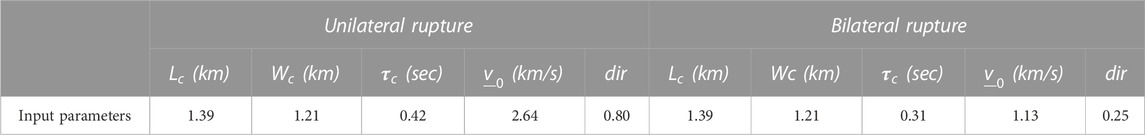
TABLE 1. Input parameters used to model the unilateral and bilateral scenarios for the characteristic rupture size (Lc and Wc), characteristic rupture duration (${\tau }_c$), centroid rupture velocity (${\underset{\_}{v}}_0$) and directivity (dir).

FIGURE 1

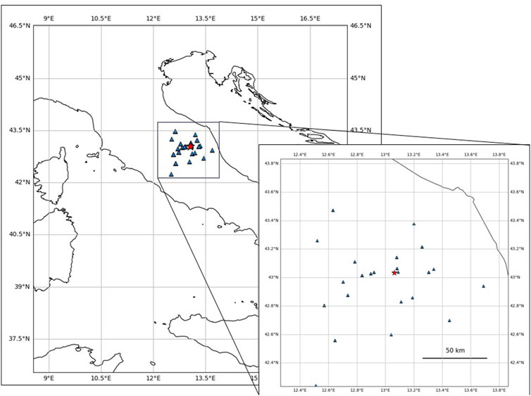
FIGURE 1. Epicentral map of the of the simulated Mw 4.6 earthquake (Lat 43.034°N, long 13.063°E, depth 5.1 km) and station configuration (triangles) used for the synthetic tests. Red star corresponds to the epicenter.

FIGURE 2

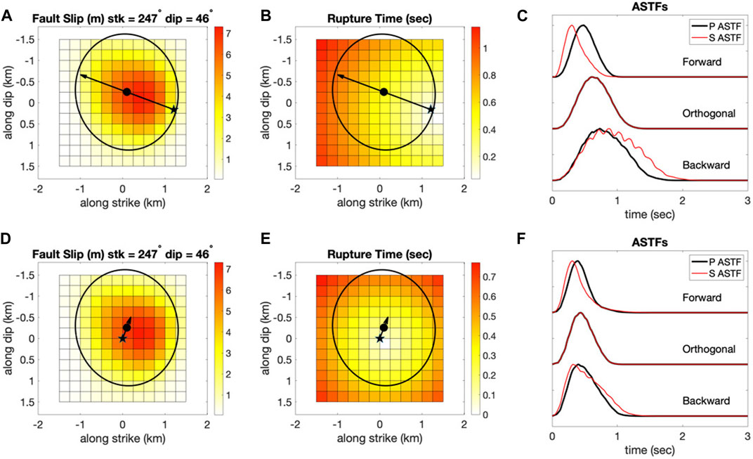
FIGURE 2. Input source for unilateral (A,B) and bilateral (D,E) scenarios. The star represents the hypocenter, the dot represents the centroid location, and the arrow indicates the rupture direction. Panels (C,F) show the ASTFs calculated from the respective models for three different azimuth directions.

FIGURE 3

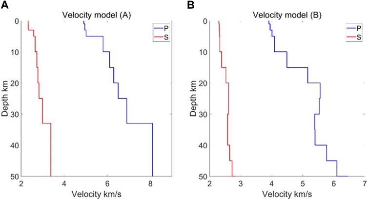
FIGURE 3. Velocity models used in this study for central Italy (Costa et al., 1993). (A) is the velocity model used to calculate the synthetic ASTFs. (B) is used to test the sensitivity of the solutions to the accuracy of the velocity model. The blue and red lines correspond to P-wave velocity and S-wave velocity, respectively.

4 Sensitivity tests

To investigate how the uncertainties introduced by the input data may affect the solutions of the resolved second seismic moments, we used the bootstrap approach. In this technique, perturbations are introduced for each input parameter to be analyzed by generating 1,000 variations around the mean. An inversion is then performed to evaluate the effects on the mean and standard deviation of the resulting data. The workflow is summarized in Figure 4. We examined the uncertainties associated with the apparent source durations ${\tau }_c\left(\underset{\_}{s}\right)$, the hypocenter location, the station distributions around the source, the focal mechanism, and the velocity model used for ray tracing. Some of these tests are interrelated. For instance, uncertainties in both the hypocenter location and the velocity model affect the calculated ray path, and both the different focal mechanism and station coverage affect the resolution of the fault plane.

FIGURE 4

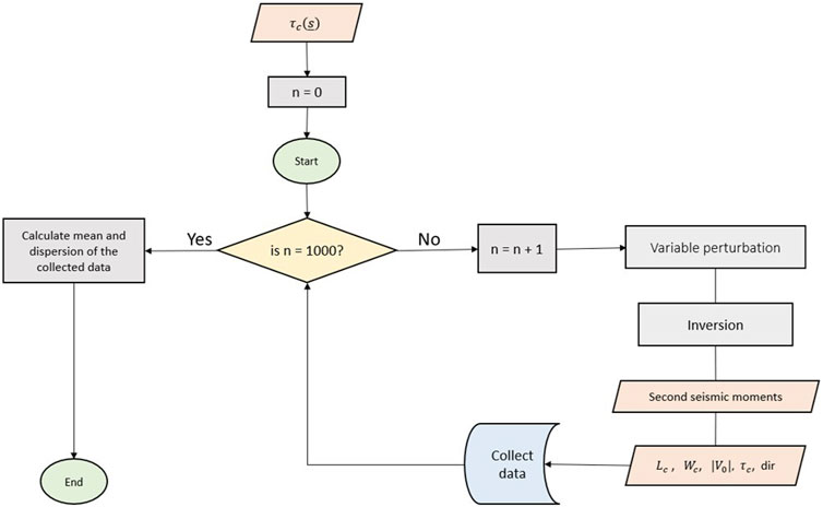
FIGURE 4. Flow chart of the perturbation tests. For each test, we calculated 1,000 random or perturbed input variables (observed ${\tau }_c$, depth, station configurations, focal mechanism, velocity model) with a given standard deviation. Then we performed the inversion and calculated the source parameters and the directivity. Finally, we calculated the mean and the dispersion of the output variables of the 1,000 scenarios.

The uncertainties in the epicenter estimates are not examined because they have negligible effects on the slowness vectors in the inversion of the second moments.

4.1 Perturbation of the apparent source duration

Potential errors in determining the duration of the ASTF, especially when the signal-to-noise ratio (SNR) is low, affect the vector b in Eq. 8.

After generating 1,000 random perturbations in the apparent source duration ${\tau }_c\left(\underset{\_}{s}\right)$ within a standard deviation set at 10% of the true value, we conducted the inversion for each perturbed ${\tau }_c\left(\underset{\_}{s}\right)$ to examine the impact of this input parameter on the inversion results.

As can be seen in Supplementary Figures S1, S2, despite the small perturbation, ${\tau }_c\left(\underset{\_}{s}\right)$ produces a large scatter of data even though the solution follows a normal distribution. In particular, an uncertainty of 10% in ${\tau }_c\left(\underset{\_}{s}\right)$ can significantly affect the characteristic rupture size and rupture velocity (Supplementary Figures S1A, B, E; Supplementary Figures S2A, B, E). The standard deviation of the resulting source duration ${\tau }_c\left(\underset{\_}{s}\right)$ seems to agree with the uncertainty caused by ${\tau }_c\left(\underset{\_}{s}\right)$ and is larger than the uncertainty caused by ${\tau }_c\left(\underset{\_}{s}\right)$ by 0.007 s and 0.005 s for the unilateral and bilateral cases, respectively.

4.2 Perturbation in the hypocentral depth

The depth of the hypocenter is one of the most important parameters, especially in real-time estimation, and its poor resolution is a recurring problem in seismology. The accuracy of hypocenter location depends mainly on the velocity model and station distribution in the near source field. An inaccurate hypocenter depth would primarily bias the slowness vector s and affect the matrix A (Eq. 8) and consequently the calculation of the second seismic moments.

To assess the robustness of the solution for the second moments, we first introduced 1,000 random perturbations of the hypocentral depth of 5.1 km with a standard deviation of 1 km. By combining all the source models from the different depth perturbations (Figures 5A, 6A), we obtained the distributions of each resolved kinematic parameter through the inversion process. Looking at the plots for the unilateral (Figures 5B–F) and bilateral scenarios (Figures 6B–F), we can see that the results of both scenarios are comparable and usually split into two distributions with a narrow spread of data (Figures 5B–D, 6B–D), except for the directivity (Figure 6E) and ${\underset{\_}{v}}_0$ of the bilateral scenario (Figure 6F) for which the position of the centroid and hypocenter are the same. The two-peaked distribution is due to the coarse discretization of the velocity model; when a smoothed velocity model is used, the two-peaked distribution is suppressed.

FIGURE 5

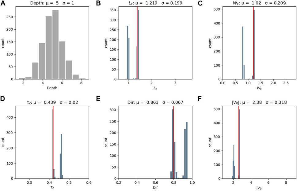
FIGURE 5. Results of the 1,000 runs of the bootstrap calculation where the original depth (5.1 km) was perturbed by a standard deviation of 1 km in the unilateral scenario. μ and σ are the mean and standard deviation for the parameters. The gray histogram (A) represents the perturbed value that is the hypocentral depth, while the blue histograms represent the solutions for the characteristic length (B), characteristic width (C), source duration (D), directivity (E) and centroid rupture velocity (F). The red lines indicate the ground truth values.

FIGURE 6

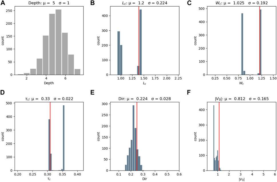
FIGURE 6. Results of the 1,000 runs of the bootstrap calculation where the original depth (5.1 km) was perturbed by a standard deviation of 1 km in the bilateral scenario. The gray histogram (A) represents the perturbed value that is the hypocentral depth, while the blue histograms represent the solutions for the characteristic length (B), characteristic width (C), source duration (D), directivity (E) and centroid rupture velocity (F). The red lines show the ground truth values.

To examine the effects of a larger error and perturbation in the velocity model, we set an average depth of 15 km. The set of depths is drawn from a Gaussian distribution with the starting depth as the mean and a standard deviation of 3 km (Figure 7A). Despite the larger standard deviation, this test generated lower dispersions of the data (Figures 7B, F) compared to the previous case. As in the previous case, the hypocenter is located on a velocity interface, but the velocity difference between the layers is smaller (Figure 3A). This is due to the higher stability in the ray path caused by the small velocity difference between the layers at a depth of 15 km. In this case, both the directivity and $\left.{\left|v\right.}_o\right|$ are overestimated.

FIGURE 7

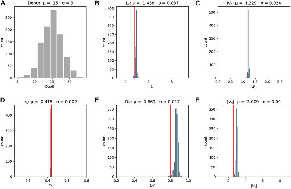
FIGURE 7. Results of inversions perturbing a hypocentral depth of 15 km by a standard deviation of 3 km in the unilateral scenario. The gray histogram (A) represents the perturbed value, while the blue histograms represent the solutions for the characteristic length (B), characteristic width (C), source duration (D), directivity (E) and centroid rupture velocity (F). The red lines show the ground truth values.

The source parameters obtained from the perturbation test of the hypocenter at a depth of 15 km do not follow a Gaussian distribution (Figure 7; Supplementary Figure S3). In particular, ${\tau }_c$, $dir$, ${\underset{\_}{v}}_0$ are the least constrained parameters.

4.3 Perturbation of the station configurations

The effects of different ray-trace coverages on our results can be studied by introducing random variations in the configuration of the recording stations that result in a significant difference in horizontal and vertical resolution. To this end, we randomly selected a fixed number of stations, for each of which we calculated a ${\tau }_c$ value from our source model (Figure 8A), and then performed the inversion. Using this approach, we investigated the effects of varying both the take-off angles and azimuthal coverage (Figure 8B) around the source.

FIGURE 8

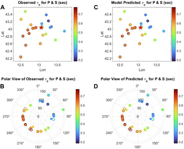
FIGURE 8. (A) Computed ${\tau }_c$ used as reference for the inverstion tests at each station. Stations are represented by dots and circles (for P- and S- waves) whose color depends on the ${\tau }_c$ value. (B) Polar view of ${\text{the}\text{reference}\mathrm{\tau }}_{\mathrm{c}}\text{ showing the azimuth and take}-\text{off angles of the ray paths from the epicenter}.$ (C) Predicted ${\tau }_c$ after performing the inversion for the unilateral scenario, and (D) polar viewof the predicted ${\tau }_c$ showing the azimuth and take-off angles of the ray paths.

First, we performed a noise-free synthetic test with good azimuthal coverage of the stations and the take-off angles between 70° and 152°. From Figures 8C, D we can see that the values of ${\tau }_c$ are accurately reproduced after the linear inversion process.

Using all stations, the results are robust for any random configuration. We then performed the bootstrap test by gradually decreasing the number of stations to achieve a tight configuration of five stations (Supplementary Figures S4, S5) out of twenty-three. The results show that the output values do not follow a normal distribution and that the dispersion of the solution obtained by randomly changing the station configuration remains quite stable compared to the other perturbation tests. In fact, the mean values are well reproduced in most cases (Table 2). This result can be attributed to the stability of the synthetic test.

TABLE 2

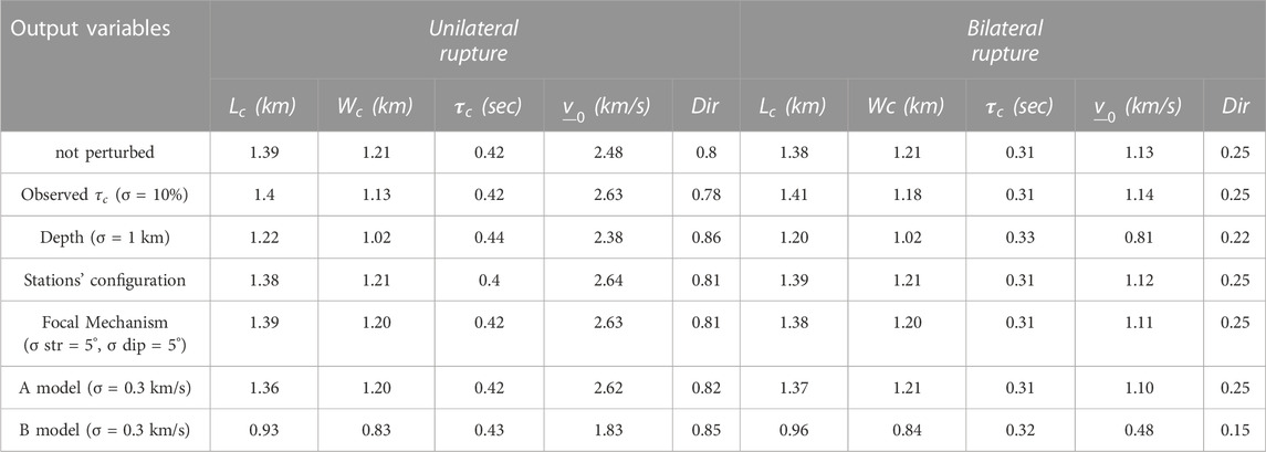
TABLE 2. Results of the mean value of each outcome variable calculated by the perturbation test for the unilateral and bilateral scenarios. For each test case, we report between brackets the standard deviation (σ) applied to the true value.

4.4 Perturbation of the focal mechanism

A change in the focal mechanism has a significant impact on the resolution of the fault plane at the recording stations, leading to potential biases in the slowness vector s and affecting the matrix A (Eq. 8).

To evaluate the effect of this factor on the solutions for the second seismic moment, we introduced a perturbation of the strike and the dip of the earthquake, within a standard deviation of 5° and treated them as two independent random variables following a Gaussian distribution. Our analysis showed that perturbing the focal mechanism had a noticeable effect on the characteristic rupture size in both scenarios, with $L_c$ varying more than $W_c$, which was found to be quite stable (Supplementary Figures S6, S7). We then used a different focal mechanism with strike and dip of 55° and 44° respectively, and a standard deviation of 10°. As in the previous case, this perturbation affects $L_c$ more than $W_c$ in both the unilateral and bilateral scenarios. The directivity is well resolved in the bilateral case, while it shows considerable variation in the unilateral case (Supplementary Figures S8, S9). In this case, the lack of bidirectional data results in a shortage of the necessary information to properly constrain directivity-related features, leading to more variable inversion results.

4.5 Uncertainty induced by the velocity model

To test the influence of the velocity model, we perturbed model A (Figure 3A), which was used to calculate the synthetic ASTFs, and model B (Figure 3B). The results show that perturbing model A by a standard deviation of 0.3 km/s does not significantly affect the solution (Supplementary Figures S10, S11). In contrast, using model B, which has lower wave velocities than model A, leads to a systematic underestimation of mean values of the rupture size and ${\underset{\_}{v}}_0$ (Supplementary Figures S12, S13).

5 Discussion and conclusion

The use of second-moment tensors to determine the source parameters, including directivity, of moderate earthquakes could be a valuable tool to improve our understanding of source dynamics in a given area and to advance disaster mitigation. A potential application of the second-moment method to small earthquakes would be to identify portions of large faults that produce supershear ruptures and correlate them with the geology of the fault zone. The second-moment method also provides lower constraints on rupture velocity, which may be particularly useful for unilateral ruptures (McGuire and Kaneko, 2018). However, before the results can be interpreted, it is necessary to know the resolution limits of the method due to the possible uncertainties of the parameters used as inputs to the computational procedure. To this end, we performed sensitivity tests of the method using synthetic ASTFs.

The sensitivity analysis performed in this study shows that the uncertainties in the input data have different effects on the calculation of the source parameters and an accurate measurement of the ASTF as well as the velocity model play the most important role in influencing the inversion process. A visual overview of the results of our tests is provided by the violin plots (Figures 9, 10) for unilateral (Figure 9) and bilateral (Figure 10) rupture scenarios. This type of plot is particularly useful for comparing the distribution of data between multiple categories or groups, as it effectively displays medians, ranges, and variabilities and facilitates comparison between different tests.

FIGURE 9

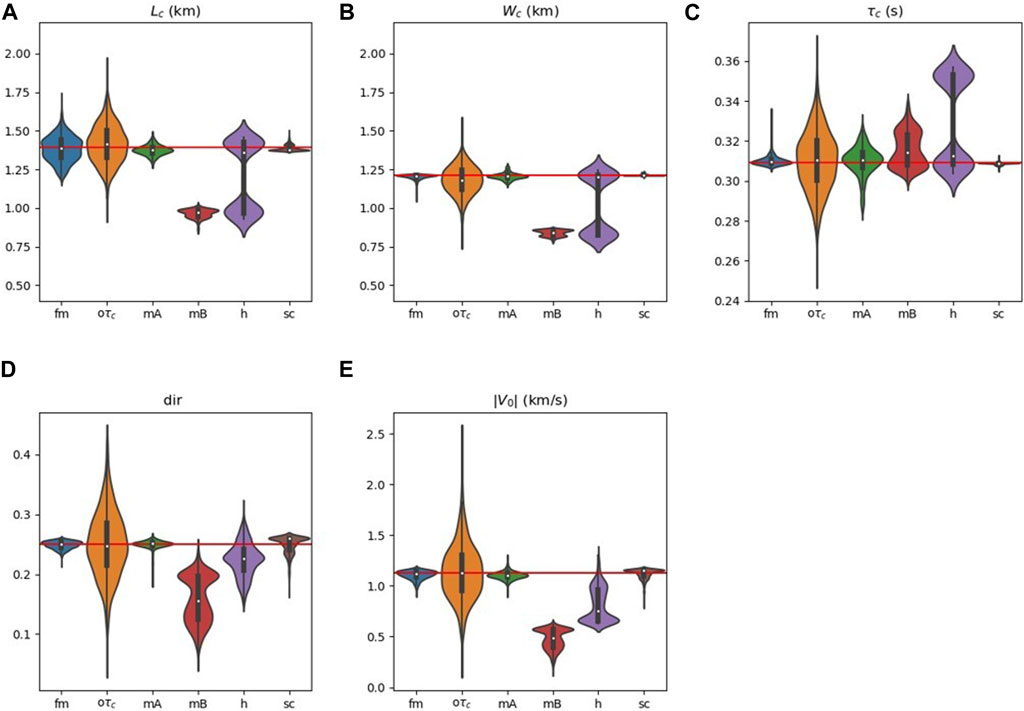
FIGURE 9. Mean values and dispersions of each output variable resulting from each perturbation test given on the x-axis, i.e., focal mechanism (fm), observed ${\tau }_c$ (o${\tau }_c$ ), velocity models (mA and mB, respectively), hypocentral depth (h), and station configuration (sc) for the unilateral scenario. (A–E) represent the solutions for the characteristic length, characteristic width, source duration, directivity and centroid rupture velocity respectively. The y-axis indicates the value of the output variable. The shape of each violin graph reflects the numerical counts of the resulting value. The red line serves as reference, indicating the input value.

FIGURE 10

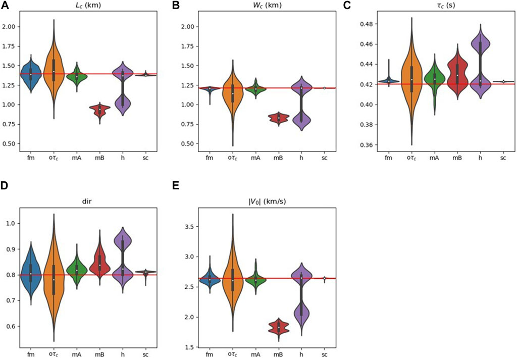
FIGURE 10. Mean values and dispersions of each output variable resulting from each perturbation test given on the x-axis, i.e., focal mechanism (fm), observed ${\tau }_c$ (o ${\tau }_c$ ), velocity models (mA and mB, respectively), hypocentral depth (h), and station configuration (sc) for the bilateral scenario. The y-axis indicates the value of the output variable. The shape of each violin graph reflects the numerical counts of the resulting value. (A–E) represent the solutions for the characteristic length, characteristic width, source duration, directivity and centroid rupture velocity respectively. The red line serves as reference, indicating the input value.

We observe that the main source parameters, i.e., rupture size, source duration, and centroid velocity, are generally well reproduced within the standard deviation. As expected, the source duration resulting from the inversion process is strongly affected by the duration of the input ASTF, and even 10% affects the inversion of the second moment tensor. This is because the ASTF is strongly related to the second moments in time, which is a vector in the inversion of the linear system (Eq. 8).

In the case of dense instrumentation, the horizontal location of the earthquake can be well resolved, but the resolution of the earthquake depth is largely determined by the velocity model, and inaccurate earthquake location can lead to uncertainties in the resolved second moments. In our case, perturbation of the hypocentral depth leads to artifacts in most of the resulting variable distributions. This is primarily due to the fact that the perturbed depth in the 1-D velocity models spans multiple layers, in which the slowness does not change once layer boundaries are crossed. In the case of model A, there is an interface between layers with a velocity difference of 0.7 km/s. As a result, the ray paths vary considerably, which shows up in the calculations as two prominent peaks in each variable distribution. Using a velocity gradient between layers, most of the parameters studied are well represented by a one-peak distribution. Care must also be taken to avoid artifacts due to the discretization of the velocity model when the hypocenter is located at an interface between two layers with high velocity contrast. A perturbation of the velocity model A by 0.3 km/s does not significantly affect the results for the fault dimension ($L_c$ and $W_c$ ). Previous studies performed by McGuire and Kaneko (2018) for various source models have shown that the fault area can be well estimated when at least 15 ASTF measurements are available at a variety of take-off angles with upward and downward rays. The exact relationship between $L_c$, $W_c$, and the total rupture dimension also depends on the particular slip distribution. McGuire and Kaneko (2018) have shown that data sets with about 30 or more measurements provide a very good recovery of the rupture velocity. We observe that the values of directivity depend on the ASTF duration, the choice of velocity model, and the focal mechanism (Figures 9D, 10D). To ensure good fault plane resolution, good ray path coverage for both upward and downward waves is critical (McGuire, 2004; McGuire and Kaneko, 2018), especially in poorly studied areas or complex geostructures. McGuire (2004) found that the horizontal component of the rupture directivities is generally well constrained and has good azimuthal coverage for strike—slip events. The component of rupture directivity along dip can only be well determined when stations directly above the hypocenter are available, since seismic rays at most other stations are nearly horizontal.

Previous research has already shown that the second-moment method can be implemented with sufficient arrays to resolve the rupture dynamics of small earthquakes (M ∼ 2.5) with high accuracy (McGuire, 2004; Fan and McGuire, 2018; Meng et al., 2020). However, in our analyses, the perturbation of the station configuration did not affect the calculation of the source parameters, due to the particular input model we considered and the accuracy of the synthetic test. Further testing using different source models and real data would be needed in the future to investigate this issue.

The choice of an inappropriate velocity model leads to a significant bias in our results, indicating the strong influence of ray path calculation in the inversion process. When we used Model B to calculate the second moments, we obtained incorrect estimates for all source parameters. In such a case, adding more stations cannot compensate for the insufficient understanding of the crustal structure (e.g., Saraò et al., 1998). Therefore, an accurate velocity model and hypocentral depth are crucial for the robustness of the results.

When using real data, the removal of path effects is also fundamental for accurate ASTF calculation and successful application of this method. If the EGF deconvolution method is used, selecting a good EGF is not an easy task. Especially for signals with low SNR, deconvolution in the frequency domain may be more advantageous. We are already working on this implementation, which will be the subject of a future publication. Although more time consuming and requiring an initial source model, we believe it would greatly improve the performance of second moments in the study of small or medium earthquakes, for which it can be difficult to find good EGFs due to noise.

Data availability statement

The original contributions presented in the study are included in the article/Supplementary Material, further inquiries can be directed to the corresponding author.

Author contributions

AC, HM, and AS conception and design of the study. AC and HM synthetic tests and visualization. AC and AS writing of the manuscript. AS, HM, and GC supervision. GC funding resources. All authors contributed to the article and approved the submitted version.

Funding

This research has been supported by the Dipartimento della Protezione Civile, Presidenza del Consiglio dei Ministri (grant no. RAN2020 - 2022 CUP J91F20000110001).

Acknowledgments

We would like to express our sincere gratitude to the editor, N.A. Pino, and the three reviewers for their time and careful review that helped us to improve the paper. This research was partly carried out in the frame of the PRIN 2022 project “2022ZHXWC9”—Intercepting the PREparatory Phase of lARge earthquakes from seismic information and gEodetic Displacement (PREPARED).

Conflict of interest

The authors declare that the research was conducted in the absence of any commercial or financial relationships that could be construed as a potential conflict of interest.

Publisher’s note

All claims expressed in this article are solely those of the authors and do not necessarily represent those of their affiliated organizations, or those of the publisher, the editors and the reviewers. Any product that may be evaluated in this article, or claim that may be made by its manufacturer, is not guaranteed or endorsed by the publisher.

Supplementary material

The Supplementary Material for this article can be found online at: https://www.frontiersin.org/articles/10.3389/feart.2023.1198220/full#supplementary-material

References

Abercrombie, R. E. (2015). Investigating uncertainties in empirical Green’s function analysis of earthquake source parameters. J. Geophys. Res. Solid Earth 120, 4263–4277. doi:10.1002/2015JB011984

CrossRef Full Text | Google Scholar

Abercrombie, R. E., Poli, P., and Bannister, S. (2017). Earthquake directivity, orientation, and stress drop within the subducting plate at the Hikurangi margin, New Zealand. J. Geophys. Res. Solid Earth 122, 10–176. doi:10.1002/2017jb014935

CrossRef Full Text | Google Scholar

Amato, A., Badiali, L., Cattaneo, M., Delladio, A., Doumaz, F., and Mele, F. M. (2006). The real-time earthquake monitoring system in Italy. Géosciences. 4, 70–75.

Google Scholar

Ammon, C. J., Velasco, A. A., and Lay, T. (1993). Rapid estimation of rupture directivity: application to the 1992 landers (MS= 7.4) and cape mendocino (M_S= 7.2), California earthquakes. Geophys. Res. Lett. 20, 97–100. doi:10.1029/92GL03032

CrossRef Full Text | Google Scholar

Beresnev, I. A. (2003). Uncertainties in finite-fault slip inversions: to what extent to believe? (A critical review). Bull. Seismol. Soc. Am. 93 (6), 2445–2458. doi:10.1785/0120020225

CrossRef Full Text | Google Scholar

Bindi, D., Pacor, F., Luzi, L., Massa, M., and Ameri, G. (2009). TheM_w6.3, 2009 L’Aquila earthquake: source, path and site effects from spectral analysis of strong motion data. Geophys. J. Int. 179, 1573–1579. doi:10.1111/j.1365-246X.2009.04392.x

CrossRef Full Text | Google Scholar

Boatwright, J. (2007). The persistence of directivity in small earthquakes. Bull. Seismol. Soc. Am. 97 (6), 1850–1861. doi:10.1785/0120050228

CrossRef Full Text | Google Scholar

Calderoni, G., and Abercrombie, R. E. (2023). Investigating spectral estimates of stress drop for small to moderate earthquakes with heterogeneous slip distribution: examples from the 2016-2017 Amatrice earthquake sequence. J. Geophys. Res. Solid Earth. 128, e2022JB025022. doi:10.1029/2022JB025022

CrossRef Full Text | Google Scholar

Calderoni, G., Rovelli, A., Ben-Zion, Y., and Di, G. R. (2015). Along-strike rupture directivity of earthquakes of the 2009 L’Aquila, central Italy, seismic sequence. Geophys. J. Int. 399-415, 399–415. doi:10.1093/gji/ggv275

CrossRef Full Text | Google Scholar

Calderoni, G., Rovelli, A., and Di Giovambattista, R. (2017). Rupture directivity of the strongest 2016–2017 Central Italy earthquakes. J. Geophys. Res. Solid Earth. 122, 9118–9131. doi:10.1002/2017JB014118

CrossRef Full Text | Google Scholar

Chimera, G., Aoudia, A., Saraò, A., and Panza, G. F. (2003). Active tectonics in Central Italy: constraints from surface wave tomography and source moment tensor inversion. Phys. Earth Planet. Int. 138, 241–262. doi:10.1016/S0031-9201(03)00152-3

CrossRef Full Text | Google Scholar

Colavitti, L., Lanzano, G., Sgobba, S., Gallovic, F., and Gallovič, F. (2022). Empirical evidence of frequency-dependent directivity effects from small-to-moderate normal fault earthquakes in Central Italy. J. Geophys. Res. Solid Earth. 127. doi:10.1029/2021JB023498

CrossRef Full Text | Google Scholar

Convertito, V., Catalli, F., and Emolo, A. (2013). Combining stress transfer and source directivity: the case of the 2012 Emilia seismic sequence. Sci. Rep. 3, 3114. doi:10.1038/srep03114

PubMed Abstract | CrossRef Full Text | Google Scholar

Convertito, V., de Matteis, R., and Pino, N. A. (2017). Evidence for static and dynamic triggering of seismicity following the 24 August 2016, MW = 6.0, Amatrice (central Italy) earthquake. Pure Appl. Geophys. 174, 3663–3672. doi:10.1007/s00024-017-1559-1

CrossRef Full Text | Google Scholar

Costa, G., Brondi, P., Cataldi, L., Cirilli, S., Ertuncay, D., Falconer, P., et al. (2022). Near-real-time strong motion acquisition at national scale and automatic analysis. Sensors 22, 5699. doi:10.3390/s22155699

PubMed Abstract | CrossRef Full Text | Google Scholar

Costa, G., Panza, G. F., Suhadolc, P., and Vaccari, F. (1993). Zoning of the Italian territory in terms of expected peak ground acceleration derived from complete synthetic seismograms. J. Appl. Geophys. 30, 149–160. doi:10.1016/0926-9851(93)90023-R

CrossRef Full Text | Google Scholar

Cultrera, G., Pacor, F., Franceschina, G., Emolo, A., and Cocco, M. (2009). Directivity effects for moderate-magnitude earthquakes (Mw 5.6–6.0) during the 1997 Umbria–Marche sequence, central Italy. Tectonophysics 476, 110–120. doi:10.1016/j.tecto.2008.09.022

CrossRef Full Text | Google Scholar

De Lorenzo, S., Filippucci, M., and Boschi, E. (2008). An EGF technique to infer the rupture velocity history of a small magnitude earthquake. J. Geophys. Res. 113, B10314. doi:10.1029/2007JB005496

CrossRef Full Text | Google Scholar

Ertuncay, D., and Costa, G. (2021). Determination of near-fault impulsive signals with multivariate naïve Bayes method. Nat. Hazards 108 (2), 1763–1780. doi:10.1007/s11069-021-04755-0

CrossRef Full Text | Google Scholar

Ertuncay, D., Malisan, P., Costa, G., and Grimaz, S. (2021). Impulsive signals produced by earthquakes in Italy and their potential relation with site effects and structural damage. Geosci 11 (6), 261. doi:10.3390/geosciences11060261

CrossRef Full Text | Google Scholar

Fan, W., and McGuire, J. J. (2018). Investigating microearthquake finite source attributes with IRIS community wavefield demonstration experiment in Oklahoma. Geophys. J. Int. 214 (2), 1072–1087. doi:10.1093/gji/ggy203

CrossRef Full Text | Google Scholar

Hartzell, S. H. (1978). Earthquake aftershocks as Green's functions. Geophys. Res. Lett. 5 (1), 1–4. doi:10.1029/GL005i001p00001

CrossRef Full Text | Google Scholar

Hough, S. E. (1997). Empirical Green's function analysis: taking the next step. J. Geophys. Res. Solid Earth. 102, 5369–5384. doi:10.1029/96JB03488

CrossRef Full Text | Google Scholar

Ji, C., Wald, D. J., and Helmberger, D. V. (2002). Source description of the 1999 Hector Mine, California, earthquake, part I: wavelet domain inversion theory and resolution analysis. Bull. Seismol. Soc. Am. 92 (4), 1192–1207. doi:10.1785/0120000916

CrossRef Full Text | Google Scholar

Kurzon, I., Vernon, F. L., Ben-Zion, Y., and Atkinson, G. (2014). Ground motion prediction equations in the San Jacinto fault zone: significant effects of rupture directivity and fault zone amplification. Pure Appl. Geophys. 171, 3045–3081. doi:10.1007/s00024-014-0855-2

CrossRef Full Text | Google Scholar

Lanza, V., Spallarossa, D., Cattaneo, M., Bindi, D., and Augliera, P. (1999). Source parameters of small events using constrained deconvolution with empirical Green’s functions. Geophys. J. Int. 137, 651–662. doi:10.1046/j.1365-246x.1999.00809.x

CrossRef Full Text | Google Scholar

Lopez-Comino, J. A., Stich, D., Morales, J., and Ferreira, A. M. G. (2016). Resolution of rupture directivity in weak events: 1-D versus 2-D source parameterizations for the 2011, M_w 4.6 and 5.2 Lorca earthquakes, Spain. J. Geophys. Res. Solid Earth. 121, 6608–6626. doi:10.1002/2016JB013227

CrossRef Full Text | Google Scholar

Mai, P. M., and Thingbaijam, K. K. S. (2014). SRCMOD: an online database of finite-fault rupture models. Seismol. Res. Lett. 85, 1348–1357. doi:10.1785/0220140077

CrossRef Full Text | Google Scholar

McGuire, J. J. (2004). Estimating finite source properties of small earthquake ruptures. Bull. Seismol. Soc. Am. 94, 377–393. doi:10.1785/0120030091

CrossRef Full Text | Google Scholar

McGuire, J. J. (2017). A MATLAB toolbox for estimating the second moments of earthquake ruptures. Seismol. Res. Lett. 88, 371–378. doi:10.1785/0220160170

CrossRef Full Text | Google Scholar

McGuire, J. J., and Kaneko, Y. (2018). Directly estimating earthquake rupture area using second moments to reduce the uncertainty in stress drop. Geophys. J. Int. 214, 2224–2235. doi:10.1093/GJI/GGY201

CrossRef Full Text | Google Scholar

McGuire, J. J., Zhao, L., and Jordan, T. H. (2001). Teleseismic inversion for the second-degree moments of earthquake space-time distributions. Geophys. J. Int. 145, 661–678. doi:10.1046/j.1365-246X.2001.01414.x

CrossRef Full Text | Google Scholar

Meng, H., and Fan, W. (2021). Immediate foreshocks indicating cascading rupture developments for 527 M 0.9 to 5.4 Ridgecrest earthquakes. Geophys. Res. Lett. 48, e2021GL095704. doi:10.1029/2021GL095704

CrossRef Full Text | Google Scholar

Meng, H., McGuire, J. J., and Ben-Zion, Y. (2020). Semiautomated estimates of directivity and related source properties of small to moderate southern California earthquakes using second seismic moments. J. Geophys. Res. Solid Earth 125, 1–21. doi:10.1029/2019jb018566

CrossRef Full Text | Google Scholar

Moratto, L., Romano, M. A., Laurenzano, G., Colombelli, S., Priolo, E., Zollo, A., et al. (2019). Source parameter analysis of microearthquakes recorded around the underground gas storage in the Montello-Collalto Area (Southeastern Alps, Italy). Tectonophysics 762, 159–168. doi:10.1016/j.tecto.2019.04.030

CrossRef Full Text | Google Scholar

Moratto, L., Santulin, M., Tamaro, A., Saraò, A., Vuan, A., and Rebez, A. (2023). Near-source ground motion estimation for assessing the seismic hazard of critical facilities in central Italy. Bull. Earthq. Eng. 21, 53–75. doi:10.1007/s10518-022-01555-0

CrossRef Full Text | Google Scholar

Moratto, L., and Saraò, A. (2012). Improving ShakeMap performance by integrating real with synthetic data: tests on the 2009 Mw = 6.3 L’Aquila earthquake (Italy). J. Seismol. 16, 131–145. doi:10.1007/s10950-011-9253-8

CrossRef Full Text | Google Scholar

Moratto, L., Saraò, A., Vuan, A., Mucciarelli, M., Jimenez, M.-J., and Garcia-Fernandez, M. (2017). The 2011 Mw 5.2 Lorca earthquake as a case study to investigate the ground motion variability related to the source model. Bull. Earthq. Eng. 15, 3463–3482. doi:10.1007/s10518-017-0110-1

CrossRef Full Text | Google Scholar

Moratto, L., Vuan, A., Sarao, A., Slejko, D., Papazachos, C., Caputo, R., et al. (2021). Seismic hazard for the trans adriatic pipeline (TAP). Part 2: broadband scenarios at the fier compressor station (Albania). Bull. Earthq. Eng. 19, 3389–3413. doi:10.1007/s10518-021-01122-z

CrossRef Full Text | Google Scholar

Moratto, L., Vuan Saraò, A., and Saraò, A. (2015). A hybrid approach for broadband simulations of strong ground motion: the case of the 2008 iwate–miyagi nairiku earthquake. Bull. Seismol. Soc. Am. 105, 2823–2829. doi:10.1785/0120150054

CrossRef Full Text | Google Scholar

Mori, J. (1993). Fault plane determinations for three small earthquakes along the San Jacinto fault, California: Search for cross faults. J. Geophys Res. Solid Earth 98 (B10), 17711–17722. doi:10.1029/93JB01229

CrossRef Full Text | Google Scholar

Mueller, C. S. (1985). Source pulse enhancement by deconvolution of an empirical Green's function. Geophys. Res. Lett. 12, 33–36. doi:10.1029/GL012i001p00033

CrossRef Full Text | Google Scholar

Rovelli, A., and Calderoni, G. (2014). Stress drops of the 1997–1998 colfiorito, Central Italy earthquakes: hints for a common behaviour of normal faults in the apennines. Pure Appl. Geophys 171 (10), 2731–2746. doi:10.1007/s00024-014-0856-1

CrossRef Full Text | Google Scholar

Saraò, A., Das, S., and Suhadolc, P. (1998). Effect of non-uniform station coverage on the inversion for earthquake rupture history for a Haskell-type source model. J. Seismol. 2, 1–25. doi:10.1023/A:1009795916726

CrossRef Full Text | Google Scholar

Shearer, P. M., Prieto, G. A., and Hauksson, E. (2006). Comprehensive analysis of earthquake source spectra in southern California. J. Geophys Res. Solid Earth 111 (B6). doi:10.1029/2005JB003979

CrossRef Full Text | Google Scholar

Silver, P. (1983). Retrieval of source-extent parameters and the interpretation of corner frequency. Bull. Seismol. Soc. Am. 73, 1499–1511. doi:10.1785/BSSA07306A1499

CrossRef Full Text | Google Scholar

Somala, S. N., Karthik Reddy, K. S. K., and Mangalathu, S. (2021). The effect of rupture directivity, distance and skew angle on the collapse fragilities of bridges. Bull. Earthq. Eng. 19, 5843–5869. doi:10.1007/s10518-021-01208-8

CrossRef Full Text | Google Scholar

Somerville, P., Graves, R. W., and Smith, N. F. (1996). Forward rupture directivity in the Kobe and Northridge earthquakes, and implications for structural engineering. Seismol. Res. Lett. 67, 55. doi:10.1111/j.1467-8624.1996.tb01877.x

CrossRef Full Text | Google Scholar

Stich, D., Mancilla, F. D. L., Baumont, D., and Morales, J. (2005). Source analysis of the M_w 6.3 2004 Al Hoceima earthquake (Morocco) using regional apparent source time functions. J. Geophys. Res. Solid Earth 110 (B6). doi:10.1029/2004JB003366

CrossRef Full Text | Google Scholar

Wang, H., Ren, Y., Wen, R., and Xu, P. (2019). Breakdown of earthquake self-similar scaling and source rupture directivity in the 2016–2017 central Italy seismic sequence. J. Geophys. Res. Solid Earth. 124, 3898–3917. doi:10.1029/2018JB016543

CrossRef Full Text | Google Scholar

Yoshida, K., and Kanamori, H. (2023). Time-domain source parameter estimation of M_W 3–7 earthquakes in Japan from a large database of moment-rate functions. Geophys. J. Int. 234, 243–262. doi:10.1093/gji/ggad068

CrossRef Full Text | Google Scholar

Yoshida, K., Uchida, N., Kubo, H., Takagi, R., and Xu, S. (2022). Prevalence of updip rupture propagation in interplate earthquakes along the Japan Trench. Earth Planet. Sci. Lett. 578, 117306. doi:10.1016/j.epsl.2021.117306

CrossRef Full Text | Google Scholar

Yue, H., Lay, T., and Koper, K. D. (2012). En échelon and orthogonal fault ruptures of the 11 April 2012 great intraplate earthquakes. Nature 490, 245–249. doi:10.1038/nature11492

PubMed Abstract | CrossRef Full Text | Google Scholar