Data-driven acoustic impedance inversion with reweighted L1 norm sparsity constraint

Acoustic impedance (AI) inversion is widely used in geophysics and reservoir prediction. But the traditional impedance inversion method cannot fully exploit the sparse characteristics of geological attributes. There are problems with multiplicity and low resolution. To solve this problem, a data-driven acoustic impedance inversion method with reweighted L1 norm constraints (DRL1) is proposed. In the inversion process, the reweighted L1 norm and local cross-correlation analysis are introduced to solve the above problems. The reweighted L1 norm is introduced as a sparse constraint (RL1) to replace the traditional inversion method which is constrained by L1 norm. The RL1 method can describe more sparsity information and improve the resolution of inversion. In addition, the quality of seismic data plays a decisive role in seismic inversion. We add local cross-correlation analysis to the inversion process. We evaluated the rationality of each sampling point in the seismic data by introducing cross-correlation analysis, controlling for their contribution to the inversion, making inversion results more stable and accurate. The inversion objective function is solved by the alternating direction multiplier method (ADMM) algorithm and soft threshold shrinkage algorithm. Finally, we validate the effectiveness of the proposed method through model tests and field data. The results show that our proposed method not only provides a more accurate portrayal of the stratigraphy, but also yields more accurate inversion results.

1 Introduction

Seismic inversion is an important method to obtain the elastic and physical properties of underground media and the properties of the fluid contained therein (Yin et al., 2015; Zong et al., 2017). In post-stack seismic inversion, impedance inversion is a common method to obtain underground impedance information (Hamid and Pidlisecky, 2015; Li et al., 2017; Wu et al., 2020). At present, there are many kinds of wave impedance inversion algorithms, such as swarm intelligence optimization algorithm, artificial intelligence algorithm, norm sparse constraint algorithm and so on. In terms of swarm intelligence optimization algorithm, Wang et al. (2017) proved the effectiveness of particle swarm optimization algorithm in wave impedance inversion. In the field of artificial intelligence, Mustafa et al. (2019) used temporal convolutional neural network models to estimate acoustic impedance from seismic data. This method can simultaneously extract low frequency and high frequency information from seismic data. Wang et al. (2019) proposed an end-to-end deep convolutional neural network inversion method for seismic acoustic wave impedance, which eliminated the dependence on wavelet estimation in the inversion process. However, the above algorithms still have some problems in the field of seismic impedance inversion, such as low accuracy and slow convergence rate.

With the continuous development of compressed sensing and sparse optimization theory, a variety of sparse forms and reconstruction algorithms have emerged, which have been applied to seismic inversion by domestic and foreign scholars to further develop the seismic inversion imaging theory (Wu, 2020). Therefore, seismic inversion algorithms with norm as sparse regularization constraint have become the focus of scholars. The Tikhonov regularization is used at the beginning of inversion, which takes the minimum L2 norm as the regularization constraint (Bickel and Martinez, 1983; Velis, 2008). Although this method can solve the instability problem of seismic inversion well, there are some problems such as low accuracy and too smooth inversion results (Berkhout, 1977). And in terms of sparse representation, the L1 norm is better than the L2 norm (Li et al., 2012; Kong et al., 2016; Chai et al., 2018). Liu et al. (2015) and Yuan et al. (2015) verify the validity of the L1 norm in inversion by using 2D model and 3D data respectively, and both confirm that the inversion method with the L1 norm as a regularization constraint has higher inversion accuracy. The L1 norm regularization method, while improving sparsity, is not the best way to perform sparse representations. On the basis of the L1 norm, one extends it to the Lp (0<p<1) quasi-norm. In terms of sparsity regularization, research shows that the Lp quasi-norm gives better results than the L1 norm (Chartrand and Yin, 2008; Mazumder et al., 2011; Li et al., 2018; Li, 2019). The Lp quasi-norm is more accurate than the L1 norm in characterizing impedance boundaries (Woodworth and Chartrand, 2016). In describing the reflection coefficient sparsity, the Lp quasi-norm is proved to be reasonable (Chen et al., 2019). Although the inversion accuracy and stability can be improved by using the above regularization constraints, the amplitude information of impedance boundary is missing, which makes the inversion result appear pseudolayer phenomenon. We introduced a reweighted L1 norm regularization inversion method to complement the impedance boundary amplitude information and thus improve the sparsity of the sparse constraint.

Despite the introduction of the more sparsity reweighted L1 norm, the most important factor affecting the inversion results is the quality of seismic data. Local cross-correlation analysis is a common way to estimate the quality of seismic data. The correlation of seismic data consists mainly of noise suppression, processing, and interpolation (Spitz, 1991; Abma and Claerbout, 1995; Wang, 2002; Liu et al., 2009; Zhang and Alkhalifah, 2019). Seismic reflection characteristics can be represented by the local correlation of neighboring seismic traces (Ma et al., 2020; Yu et al., 2020). Based on the local correlation constraint, a new inversion method is proposed, which can effectively improve the convergence and multi-solution of geophysical inversion (Yin et al., 2018). Yin et al. (2020) performed local cross-correlation analysis on seismic data, discards unreasonable seismic data sampling points, and the inversion parameters at the abandoned points are corrected by neighboring seismic traces.

In this paper, a data-driven acoustic impedance inversion method is raised by combining two methods of reweighted L1 norm regularization and local cross-correlation analysis. The algorithm is implemented in 3D field-data. First, in sparse constraint terms, we use the reweighted L1 norm with better sparsity to replace the traditional L1 norm constraint, which improves the resolution of inversion results. Secondly, considering the impact of seismic data quality on the inversion results, we evaluate the reliability of each sampling point through local correlation analysis to control their contribution to the inversion, resulting in more stable and accurate inversion results. Then, the alternating direction multiplier method (ADMM) algorithm is introduced to decompose the multi-parameter inversion problem into multiple single-parameter sub-problems that are easy to solve (Esser, 2009; Boyd et al., 2011; Ghadimi et al., 2014). The soft threshold shrinkage algorithm is introduced to solve the mixed norm optimization problem. Finally, in this paper, the inversion results of the method are compared with the traditional L1 norm constraint method by model tests and field-data. The results indicate that the presented method has higher stability and resolution, and provides a more accurate portrayal of the strata.

2 Methodology

2.1 Traditional inversion objective function

Under the assumption of linear system, seismic records can be written into the form of seismic wavelet and formation reflection coefficient convolution (Robinson, 1967):

$S=W*R+n(1)$

where S, W, n and R denote the seismic data, the wavelet, the random noise and the reflection coefficient, respectively.

The linear relationship between the impedance and the reflection coefficient can be written as:

$R_i=\frac{Z_{i+1}-Z_i}{Z_{i+1}+Z_i}\approx \frac{1}{2}\Delta \ln Z_i=\frac{1}{2}\Delta \left(\ln Z_{i+1}-\ln Z_i\right)(2)$

where $Z_i$ is the impedance value between $i^{th}$ layer and ${\left(i+1\right)}^{th}$ layer. △ shows the increment.

$\underset{S}{\underset{}{\left[\begin{array}{c}{S}_1\\ S_2\\ ⋮\\ S_N\end{array}\right]}}=\underset{W}{\underbrace{\left[\begin{array}{c}{W}_1\\ W_2\\ \begin{array}{c}⋮\\ W_l\\ \\ \end{array}\\ \end{array}\begin{array}{c}\\ W_1\\ \begin{array}{c}{W}_2\\ ⋮\\ W_l\\ \end{array}\\ \end{array}\begin{array}{c}\\ \\ \begin{array}{c}\ddots \\ \ddots \\ \ddots \\ \ddots \end{array}\\ \end{array}\begin{array}{c}\\ \\ \begin{array}{c}\\ W_1\\ W_2\\ ⋮\end{array}\\ W_l\end{array}\right]}}\underset{D}{\underbrace{\frac{1}{2}\left[\begin{array}{c}-1\\ \\ \\ \end{array}\begin{array}{c}1\\ -1\\ \\ \end{array}\begin{array}{c}\\ 1\\ \ddots \\ \end{array}\begin{array}{c}\\ \\ \ddots \\ -1\end{array}\begin{array}{c}\\ \\ \\ 1\end{array}\right]}}\underset{L}{\underbrace{\left[\begin{array}{c}\ln \left(Z_1\right)\\ \ln \left(Z_2\right)\\ ⋮\\ \ln \left(Z_N\right)\end{array}\right]}}+n(3)$

Let $L=\ln Z$. So, the simplified form is as follows:

$S=WDL+n(4)$

where $S_i$ is the seismic record at the $i^{th}$ sampling point of a seismic track. D represents the matrix of difference. L represents the logarithmic acoustic impedance.

In inversion, the relationship is described between impedance and seismic data by the fidelity term (Li et al., 2018):

$J\left(L\right)=\underset{L}{\min }{‖S-WDL‖}_2^2(5)$

where ${‖‖}_2^2$ represents the L2 norm. W represents the wavelet kernel matrix. D denotes the matrix of difference. L represents the logarithmic form of acoustic impedance.

The inversion efficiency can be improved by introducing the initial model constraint. And since DL is sparse, we can constrain it with the L1 norm:

$J\left(L\right)=\underset{L}{\min }{‖S-WDL‖}_2^2+\lambda {‖DL‖}_1^1+\alpha {‖L-L_0‖}_2^2(6)$

where $\alpha$ and $\lambda$, respectively, represent the weight coefficient of the reflection coefficient and the initial model. $L_{\mathbf{0}}$ represents the initial model, ${‖‖}_1^1$ represents the L1 norm.

2.2 Reweighted L1 norm inversion (RL1)

The reweighted L1 norm is a generalization of the L1 norm, Candes et al. (2008) verified that the reweighted L1 norm is better than the L1 norm in terms of sparsity representation. Both are defined as follows:

${‖r‖}_1^1={\displaystyle \sum _{i=1}^{n-1}}\left|r_i\right|(7)$

${‖Mr‖}_1^1={\displaystyle \sum _{i=1}^{n-1}}\left|m_i{r}_i\right|(8)$

where $m_i$ and $r_i$ represent the weighting factor and the reflection coefficient, respectively. M represents the reweighted matrix, and the expressed is:

$M=\left[\begin{array}{ccccc}{m}_1& 0& \cdots & \cdots & 0\\ 0& \ddots & \ddots & \ddots & ⋮\\ ⋮& \ddots & m_i& \ddots & ⋮\\ ⋮& \ddots & \ddots & \ddots & 0\\ 0& \cdots & \cdots & 0& m_{n-1}\end{array}\right](9)$

The relation between reflection coefficient $r$ and $m_i$ is:

$m_i=\frac{1}{\left|r_i\right|+\epsilon }(10)$

where $\epsilon$ represents the adjustment factor to ensure the stability of $m_i$.

Here, we use reflection coefficient optimization problem to quantitatively evaluate the sparsity of reweighted L1 norm and L1 norm:

$J\left(r\right)=\underset{r}{\min }{‖r‖}_1^{1}s.t.{‖r-r_0‖}_2^2<Er{r}^2(11)$

$J\left(r\right)=\underset{r}{\min }{‖Mr‖}_1^{1}s.t.{‖r-r_0‖}_2^2<Er{r}^2(12)$

where $r_0$ denotes the true reflection coefficient. Where $Err$ denotes positive numbers close to zero.

Figure 1 presents the results of the optimization problems, where red circle represents ${‖r-r_0‖}_2^2$, the blue rectangle represents the sparse term, and the intersection of the first two represents the reflection coefficient solution. From Figure 1, We can see clearly, the reweighted L1 norm than L1 norm has better sparse. It is therefore concluded that the reweighted L1 norm is a good description of the sparsity of the reflection coefficients.

FIGURE 1

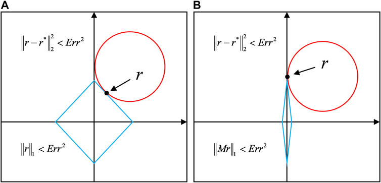
FIGURE 1. The sparsity test results. (A) L1 norm; (B) Reweighted L1 norm.

We introduce the reweighted L1 norm into the objective function, then (6) can be written as:

$J\left(L,R\right)=\underset{L,R}{\min }{‖S-WDL‖}_2^2+\lambda {‖R‖}_1^1+\alpha {‖L-L_0‖}_2^{2}s.t.R=MDL.(13)$

2.3 Data-driven Reweighted L1 norm inversion (DRL1)

In seismic inversion, the most important factor affecting the inversion results is the quality of seismic data, which immediately affects accuracy and resolution of inversion. So, on the basis of the reweighted sparse constraint, we add the correlation analysis of seismic data. The correlation analysis formula is:

$C_{i,j}=\frac{\left|{\displaystyle \sum _{\tau =-w}^w}s\left(i-\tau ,j\right)s\left(i-\tau +u,j^{\prime }\right)\right|}{\sqrt{{\displaystyle \sum _{\tau =-w}^w}{s}^2\left(i-\tau ,j\right)s^2\left(i-\tau +u,j^{\prime }\right)}}(14)$

where s represents the seismic data. C denotes the local correlation coefficient. i and j denote the number of sampling point and the number of traces respectively. $j^{\prime }$ is the neighboring seismic trace of j. The w denotes the time window used for the calculation of the correlation coefficient. U denotes the upward and downward drift times of the sampling and analysis points used for correlation analysis within adjacent seismic traces, let $u\in \left[-22\right]$ in this paper. Correlation analysis of adjacent seismic tracks is shown in Figure 2. As shown in Figure 2, the yellow analysis point can be represented as $s\left(i,j\right)$, the time window for correlation analysis $w=3$, the relative position relationship between grey point $s\left(i-2,j-1\right)$ and analysis points can be represented by $u=-2$, and the relative position relationship between green point $s\left(i+2,j+1\right)$ and analysis points can be represented by $u=2$.

FIGURE 2

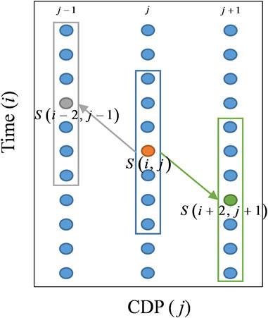
FIGURE 2. Correlation analysis diagram of neighboring seismic traces.

We calculate the number of cross-correlation coefficient for each u and use the biggest value for that point to be the correlation coefficient. Usually, we discard sample points with low local cross-correlation coefficient, which are thought unreasonable. The representation is as follows:

$H_{i,j}=\left\{\begin{array}{cc}0,& C_{i,j}<C_0\\ C_{i,j},& C_{i,j}>C_0\end{array}\right.(15)$

where $H_{i,j}$ is the local optimization operator, which serves to reduce the contribution of less correlated regions of the seismic data to the inversion results or to discard them directly. C₀ is the threshold related to the local cross-correlation coefficient.

$H$ is introduced into the objective function, thus controlling the contribution of each sampled point in the seismic data to the inversion. The reconstruction of the seismic record is as follows:

$S^{\prime }=H\mathrm{o}\left(S\right)(16)$

where the symbol “o" represents the “Hadamard product” operator,” which denotes the multiplications of the corresponding points of two matrices with the identical rows and columns. $S^{\prime }$ represents the reconstructed synthetic seismic records.

The objective function of the presented methods is:

$\begin{array}{l}J\left(L,R,S_r\right)=\underset{L,R,s_r}{\min }{‖H\mathbf{o}\left(S-S_r\right)‖}_2^2+\lambda {‖R‖}_1^1+\alpha {‖L-L_0‖}_2^2\\ s.t.S_r=WDL,R=MDL.\end{array}(17)$

To solve the objective function, we use ADMM to transform it into several linear sub-problems to solve. Further, the dual term is introduced to transform the constrained objective function Eq. 17 into an unconstrained objective function, and the following is obtained:

$\begin{array}{l}J\left(L,R,C_1,C_2,S_r\right)=\underset{L,R,C_1,C_2,S_r}{\min }{‖H\mathbf{o}\left(S-S_r\right)‖}_2^2+\lambda {‖R‖}_1^1+\alpha {‖L-L_0‖}_2^2+\mu {‖R-MDL-C_1‖}_2^2+\gamma {‖S_r-WDL-C_2‖}_2^2\\ s.t.S_r=WDL,R=MDL.\end{array}(18)$

where $\gamma$ and $\mu$ represents the weighting factor of the dual variable.

The sub-problems associated with L are represented as follows:

$J\left(L\right)=\underset{L}{\min }\alpha {‖L-L_0‖}_2^2+\mu {‖R-MDL-C_1‖}_2^2+\gamma {‖S_r-WDL-C_2‖}_2^2(19)$

Eq. 19 contains only L2 norm, which is a convex optimization problem. Therefore, taking the gradient of L and simplifying it, we can get:

$L^{i+1}={\left(\gamma G^{T}G+\alpha E+\mu D^T{M}^{iT}{M}^{i}D\right)}^{-1}\left[\alpha L_0+\mu D^T{M}^{iT}\left(R^i-C_1\right)+\gamma G^T\left(S_r^i-C_2\right)\right](20)$

Where $i+1$ shows the ${\left(i+1\right)}^{th}$ iteration. G represents $G=WD$. E represents the identity matrix.

The sub-problem of R is expressed as:

$J\left(R\right)=\underset{R}{\min }\lambda {‖R‖}_1^1+\mu {‖R-MDL-C_1‖}_2^2(21)$

For the above sub-problem, the soft threshold shrinkage algorithm (Chartrand and Yin, 2016) is adopted to solve it:

$R^{i+1}=\max \left(\left|M^{i}D{L}^{i+1}+C^i\right|-\lambda /\mu ,0\right)*sign\left(M^{i}D{L}^{i+1}+C^i\right)(22)$

where $sign$ can be expressed as:

$sign\left(x\right)=\left\{\begin{array}{cc}-1,& x<0\\ 0,& x=0\\ 1,& x>0\end{array}\right.(23)$

The sub-problems associated with $S_r$ are represented as follows:

$J\left(S_r\right)=\underset{S_r}{\min }{‖H\mathbf{o}\left(S-S_r\right)‖}_2^2+\gamma {‖S_r-WDL-C_2‖}_2^2(24)$

Expand the above formula and compute the gradient of $S_r$ to obtain:

$S_r^{i+1}=\left(H\mathbf{o}H\mathbf{o}S+\gamma G{L}^{i+1}+\gamma C_2^i\right)./\left(H\mathbf{o}H+\gamma E_1\right)(25)$

where $E_1$ represents the identity matrix. $./$ represents the division the corresponding points of two matrices with the identical rows and columns.

The sub-problems associated with $C_1,C_{\mathbf{2}}$ are represented as follows:

$J\left(C_1\right)=\underset{C_1}{\min }\mu {‖R-MDL-C_1‖}_2^2(26)$

$J\left(C_2\right)=\underset{C_2}{\min }\gamma {‖S_r-WDL-C_2‖}_2^2(27)$

After the expansion of these two sub-problems, the gradient of $C_1$ and $C_2$ is obtained:

$C_1^{i+1}=C_1^i+\left(M^{i}D{L}^{i+1}-R^{i+1}\right)(28)$

$C_2^{i+1}=C_2^i+\left(G{L}^{i+1}-S_r^{i+1}\right)(29)$

Finally, update the reweight matrix with $L^{i+1}$:

$M_j^{i+1}=\frac{1}{\left|n_j^{i+1}\right|+\epsilon }s.t.n=DL.(30)$

We summarized the above inversion steps and obtained the seismic acoustic impedance inversion framework based on DRL1 as follows:

Algorithm 1. Seismic acoustic impedance inversion method based on DRL1

1. Initialize: $L^0=L_0$, $S_r^0=G{L}_0$, $R^0=0$, $C_1^0=0$, $C_2^0=0$, $M^0=E$, the threshold value ${\epsilon }_0$.

2. while: ${‖L^{i+1}-L^i‖}_2/{‖L^i‖}_2>{\epsilon }_0$ do.

3. Update $L^{i+1}$ according to Eq. 20

4. Update $R^{i+1}$ according to Eq. 22

5. Update $S_r^{i+1}$ according to Eq. 25

6. Update $C_1^{i+1}$ , $C_2^{i+1}$ according to Eqs 28, 29

7. Update $M^{i+1}$ according to Eq. 30

8. $i=i+1$.

9. end

Output: $AI=\exp \left(L^{i+1}\right)$.

3 Model testing

3.1 Noiseless model testing

Here, we introduce the Marmousi2 model to test the feasibility of the methods in this paper. In Figure 3A, the AI model size is 500 traces with 380 points per trace. Beyond that, Figure 3B show the initial model, which is obtained by Gaussian filtering. The RL1 method and the L1 method are tested separately under the condition of noiseless. Figures 4A, C respectively show the inversion results of the two methods under optimal parameters. The inversion results of the two methods are close to the real model, and the difference cannot be directly seen. Therefore, the absolute errors of the two inversion results were obtained respectively (Figures 4B, D). The results show that the reweighted L1 norm has a good inhibition effect on the pseudo-layer phenomenon. Moreover, from the perspective of inversion precision, the reweighted L1 norm constraint has higher accuracy than the L1 norm constraint.

FIGURE 3

FIGURE 3. (A) The true AI model (B) The initial AI model.

FIGURE 4

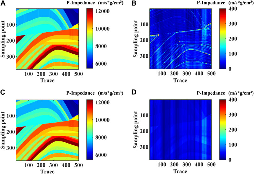
FIGURE 4. (A) The results based on L1 norm constraint method. (B) The absolute error based on L1 norm constraint method. (C) The result based on RL1 method. (D) The absolute error based on RL1 method.

To quantitatively analyze the inversion effects of the two methods, the inversion results of the 125th and the 325th traces are extracted (Figure 5). Where, black line represents the true impedance value, red line represents the reweighted L1 norm constrained inversion results, green line represents the L1 norm constrained inversion results, and the dotted line represents the initial model. Both the blue line and the green line are close to the black line, but the blue line is closer to the change trend of the true impedance, indicating that the reweighted L1 norm has better inversion effect. By enlarging part of the single trace inversion results (at the black arrow), it can be seen that the pseudo-layer phenomenon exists in the inversion results constrained by L1 norm. However, the stratigraphic characterization of the inversion results of the reweighted L1 norm is clear, which can suppress the pseudo-layer phenomenon strongly.

FIGURE 5

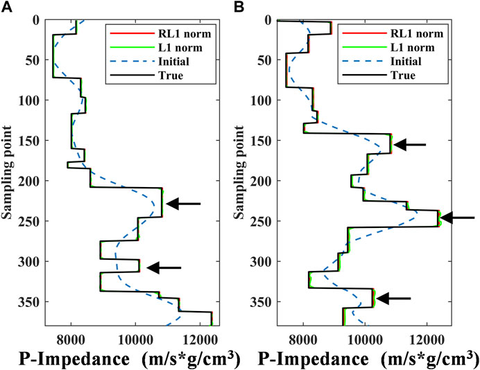
FIGURE 5. The single trace result: (A) trace 125. (B) trace 325.

3.2 Noise model testing

The quality of seismic data is still the basic factor affecting inversion. The contribution of unreasonable seismic data is reduced or abandoned by local cross-correlation analysis and the contribution of seismic data from each sampling point is controlled. Finally, adjacent seismic tracks are used to correct or recover the inversion parameters at the points where contributions are reduced or dropped. Therefore, the stability of inversion results can be improved by local cross-correlation analysis in the seismic data area which is seriously disturbed by noise. As shown in Figure 6A, the synthetic seismic record was obtained by combining reflection coefficient and wavelet. And the dominant frequency of the wavelet is 30 Hz. Figure 6B is the zoomed-in view of the dashed box in Figure 6A. In Figure 6C, 10% Gaussian white noise is added to obtain the synthetic seismic record containing noise. Figure 6D is the zoomed-in view of the dashed box in Figure 6C. We can see that the seismic traces are heavily influenced by noise interference. Through local cross-correlation analysis of seismic data, we use Eq. 16 to obtain the reconstructed synthetic seismic records (Figure 6E). We can see from Figure 6F that the reconstructed synthetic seismic record reduces the influence of low correlation regions, such as those subject to noise interference, on the inversion result.

FIGURE 6

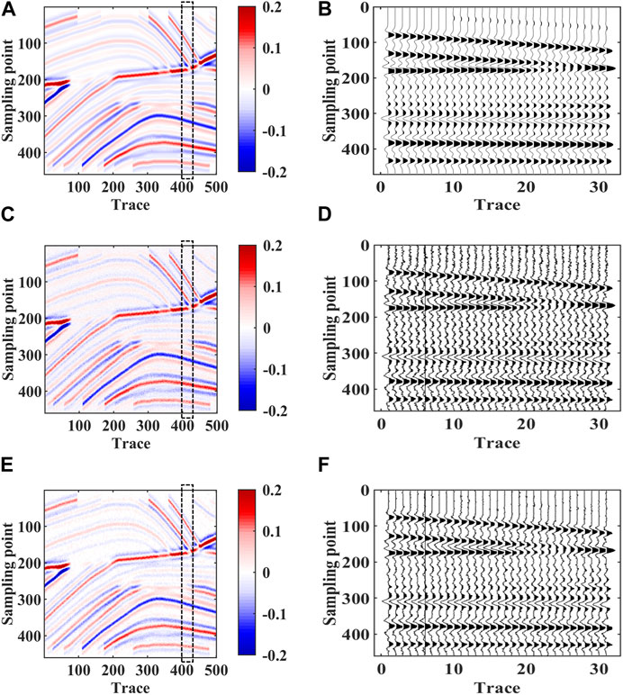
FIGURE 6. The seismic data: (A) Synthetic seismic recordings without noise. (B) Zoomed-in display at the dotted box of the without noise-containing seismic record. (C) Synthetic seismic recordings with noise. (D) Zoomed-in display at the dotted box of the noise-containing seismic record. (E) Synthetic seismic recordings after the cross-correlation processing. (F) Zoomed-in display at the dashed box after the cross-correlation processing.

The C₀ in Eq. 15 is very important for local cross-correlation analysis of synthetic seismic records. Too small C₀ cannot effectively reduce the influence of low correlation areas in seismic data, such as severe noise interference and extreme discontinuity, on the inversion results. If C₀ is too large, valid information cannot be retained. Therefore, in order to achieve the optimal inversion result, a suitable threshold C₀ should be found. After obtaining the reconstructed synthetic seismograms with different thresholds C₀, we use SNR (Signal Noise Ratio) and RMSE (Root Mean Square Error) to quantitatively analyze the reconstructed results. As shown in Figure 7, with the increase of C₀, SNR gradually increases and RMSE gradually decreases. When C₀>0.6, SNR began to decrease and RMSE began to increase. Therefore, when C₀=0.6, the reconstructed synthetic seismic record reaches the optimum. We apply the reconstruction results when C₀ = 0.6 to the subsequent inversion.

FIGURE 7

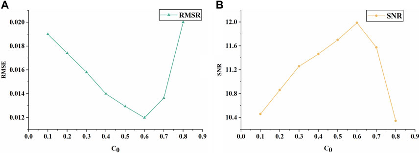
FIGURE 7. Quantitative analysis of C₀: (A) RMSE. (B) SNR.

In Figure 8, we take the inversion method based on L1 norm constraint as a conventional method and compare it with the RL1 method and the DRL1 method proposed. Because of the addition of 10% noise, three method shows the phenomenon of “ vertical striping.” The inversion results show that the DRL1 method is less affected by noise than the conventional method and the RL1 method, and the inversion section boundary is clearer and the inversion results are more accurate. To show the effect of the different methods more clearly, we combine the inversion result of the three method and the theoretical model, and get the absolute error. By comparing Figures 8B, D, F, we can see that the inversion effect of the three inversion methods is not good at the interlace position. But the absolute error of the method in this paper is smaller, which indicates that the introduction of local cross-correlation analysis can reduce the inversion instability at the interlace position and thus improve the inversion accuracy. However, there are still some problems in Figure 8F, including transverse discontinuities. We will address these questions later in our research. And we show in Table 1 the optimal parameters for the different inversion methods.

FIGURE 8

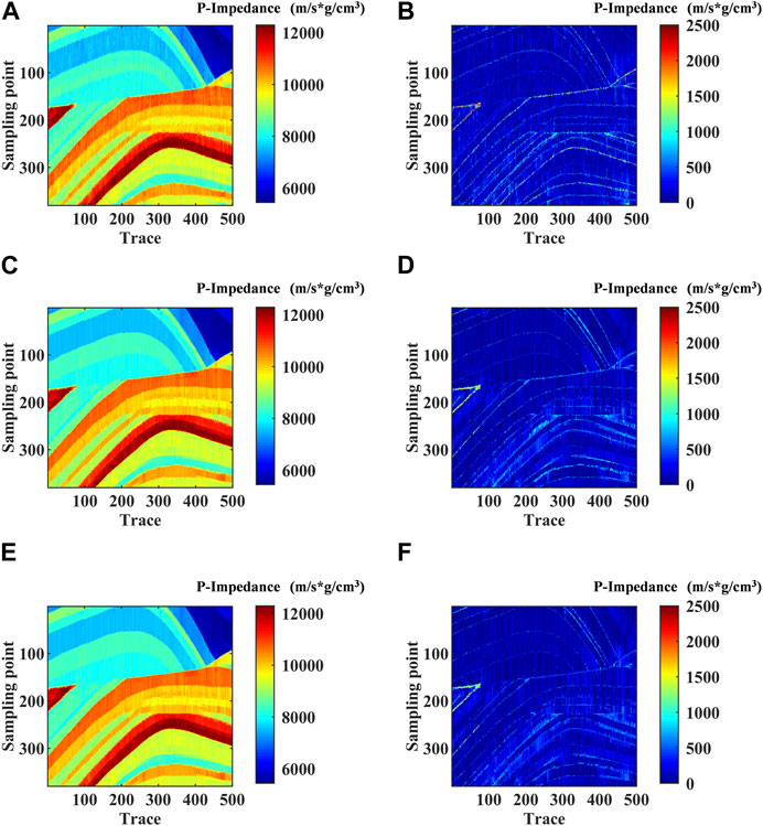
FIGURE 8. (A) The results based on L1 norm constraint method; (B) The absolute error based on L1 norm constraint method; (C) The result based on RL1 norm constraint method; (D) The absolute error based on RL1 norm constraint method; (E) The result based on our proposed method; (F) The absolute error based on our proposed method.

TABLE 1

TABLE 1. Optimal parameter set for model data.

In addition, we obtained histograms of the residual distribution corresponding to the inversion results for the three inversion methods (Figure 9), so as to quantitatively evaluate the advantages and disadvantages of the methods. In Figure 9, black represents the error curve of the L1 norm constrained method, blue represents the error curve of the RL1 norm constrained method, and red represents the error curve of the proposed method. By comparing the three curves, it can be seen that the area covered under the red curve is smaller than the black curve and the blue curve, indicating that the inversion error of the proposed method is smaller and the accuracy is higher.

FIGURE 9

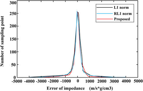
FIGURE 9. Histogram of residual distribution.

In order to compare the gaps of the inversion results in more detail, we extracted the single-trace data of the inversion results for comparison, which is shown in Figure 10. The results show that the red and blue lines can better restore the stratigraphic information and suppress the pseudo-layer phenomenon compared with the green line (Figure 10 black arrows indicated). Further comparing the results of the red and blue lines, we find that the red line is closer to the real impedance, indicating that the local cross-correlation analysis can indeed improve the accuracy and stability of the inversion. Therefore, it is verified that our method can reduce the multiple solutions of the inversion problem and enhance the inversion precision.

FIGURE 10

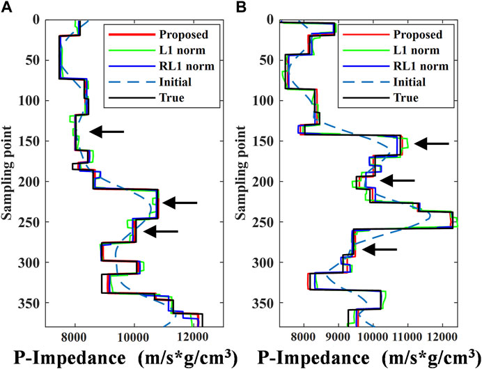
FIGURE 10. The single trace result: (A) trace 125. (B) trace 325.

To give the readers a clearer understanding of the role of each parameter in the proposed method. We quantitatively evaluated the signal-to-noise ratio (SNR) of different parameter inversion results. The SNR is defined as follows:

$SNR=10*\lg \frac{{‖Z^t-\overline{Z}‖}_2^2}{{‖Z^{inv}-\overline{Z}‖}_2^2}(31)$

where $Z^t$ represents the model of acoustic impedance. $\overline{Z}$ represents mean value of model acoustic impedance. $Z^{inv}$ represents the estimated acoustic impedance result.

We analyzed the performance of the parameters (α, γ, μ, λ) of the proposed method. α is the weight coefficient of the initial model, which determines the similarity between the inversion results and the initial model. However, the weight of the initial model in the inversion should not be too large, otherwise the inversion results will be close to the initial model. We selected five points for each parameter and calculated their SNR. From Table 2, we can see that when α=3×10⁻³, we can get the best inversion result.

TABLE 2

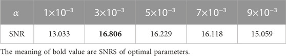
TABLE 2. Quantitative comparison of different α.

The μ, γ denote the degree of fitting of the reflection coefficient R to the MDL and the degree of fitting of the seismic record S_r to the WDL, respectively. From Tables 3, 4, we can see that we can get the best inversion results when μ=1 × 10⁻⁵ and γ=4 × 10⁻¹.

TABLE 3

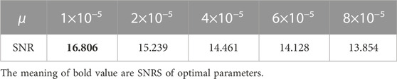
TABLE 3. Quantitative comparison of different μ.

TABLE 4

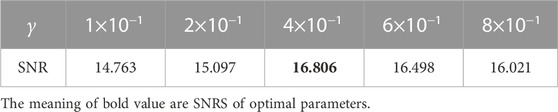
TABLE 4. Quantitative comparison of different γ.

The λ denotes the weight of sparse constraint terms of the reweighted L1 norm in the objective function. As can be seen from Table 5, the SNR increases first and then decreases with the increase of λ. The best result is obtained when λ=2 × 10⁻⁶.

TABLE 5

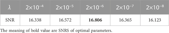
TABLE 5. Quantitative comparison of different λ.

3.3 Field-data example

Similarly, the proposed method is applied to real seismic data. Field-data are obtained from the southern Sichuan Basin. Figure 11A shows a seismic profile of the actual data, with a size of 300 traces, 190 points per trace, and a sampling interval of 2 ms. And the black line in the diagram shows the location of well A. The initial model of AI is shown in Figure 11B.

FIGURE 11

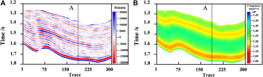
FIGURE 11. Original data: (A) Field seismic profiles. (B) The initial AI model.

We take the method based on L1 norm constraint as a conventional method and compare it with the RL1 method and DRL1 method in this paper, as shown in Figures 12A–C. From the black boxes and arrows, the proposed DRL1 method has a stronger sense of layering and higher resolution compared with the traditional method and RL1 method. And the whole impedance profile has a better lateral continuity. Second, by comparing the matching degree of well curve in section, it can be seen that the three methods can well match well curve on the whole, but in some small and thin layers, the matching degree of inversion section and well curve of the proposed method is better. Therefore, it is verified that the reweighted L1 norm can better describe the sparse information than the L1 norm, and the stratigraphic characterization is more clearly. Based on the RL1 method, the inversion results are more continuous and accurate after further local correlation analysis.

FIGURE 12

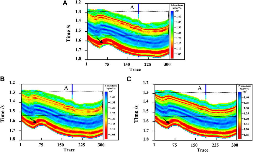
FIGURE 12. Comparison of inversion results of different methods: (A) The results based on L1 norm constraint method. (B) The results based on reweighted L1 norm constraint method. (C) The results based on our proposed method.

As shown in Figure 13, in order to compare the inversion results of the three methods more visually, we extracted the well bypass seismic traces obtained from the inversion results of the three methods respectively and compared them with the AI calculated from the logging curves. In Figure 13, the black line is the wave impedance data, the green line is the inversion result of L1 norm method, the blue line is the inversion result of RL1 norm method, and the red line is the inversion result of DRL1 method. The red line in Figure 13A is closest to the black line, and the red line is closer to the zero value of 0 in Figure 13B, which verifies that our proposed method yields smaller errors and higher inversion accuracy compared to the other two methods.

FIGURE 13

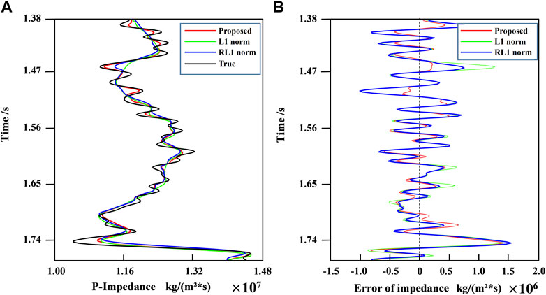
FIGURE 13. Comparison of well bypass: (A) The inversion results. (B) The residual of impedance.

In the previous part, we verified the good applicability of the proposed method in real data by two-dimensional profile. Therefore, we extend the method to 3D space to further verify its applicability. Figure 14A shows the 3D distribution of the real post-stack seismic data set. Figures 14B–D shows the 3D distribution of the inversion result of the conventional method, RL1 method and the DRL1 method. As per the obtained results, when compared with the conventional method and RL1 method, the DRL1 method improves the robustness of the inversion results and makes them more continuous in space. In Figures 14B–D, it is clear from the black arrow mark that the DRL1 method is more precise in depicting thin layers and has better continuity in 3D space.

FIGURE 14

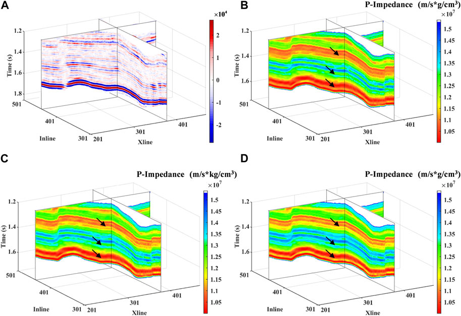
FIGURE 14. The 3D distribution of original data and inversion results by different methods: (A) Real post-stack seismic data set. (B) The results based on L1 norm constraint method. (C) The results based on reweighted L1 norm constraint method. (D) The results based on our proposed method.

4 Discussion

The inverse problem is a painful ordeal for the impatient, but for those who love it, it is a thrilling challenge. This is because the process of getting to the final result is tedious and requires repeated testing. For example, the inversion objective function in Eq. 18 has many parameters that affect the inversion result, and we need to make them get the optimal parameters so as to get the best inversion result. The following is a brief discussion of each parameter. First, the degree of similarity between the inversion results and the initial model is determined by $\alpha$. The more credible the initial model, the larger $\alpha$ can be set. The degree of fitting between the reflection coefficient $R$ and MDL depends on the parameter $\mu$, the larger $\mu$, the higher the degree of fitting. The parameter $\gamma$ is used to define the fitting relationship between the seismic record $S_r$ and WDL, and the fitting degree depends on the size of $\gamma$. The $\lambda$ determines the weight of the reweighted L1-norm sparse constraint term in the objective function. The larger the noise in seismic data, the larger the value of $\lambda$ should be. However, if the value is too large, the inversion result will deviate from the real value. In general, in inverse problems, the optimal parameters are not unique, but knowing the role of each parameter will help us get better inversion results faster.

5 Conclusion

In this paper, a data-driven acoustic impedance inversion way is introduced. The RL1 algorithm applies the reweighted L1 norm with good sparsity as the sparsity constraint, which improves the precision of inversion results and makes the characterization of stratigraphic horizon clearer. On the basis of RL1 algorithm, DRL1 algorithm is further proposed to reconstruct seismic data through local cross-correlation analysis, so as to control the proportion of each point in the inversion process and decrease the influence of unreasonable points on the inversion results. ADMM algorithm and soft threshold shrinkage algorithm are used to solve the inversion problem. Finally, through model tests and field data examples, it is verified that the proposed method has higher inversion precision than the general methods. In particularly, in seismic data with severe noise interference, the proposed method can achieve better inversion results than conventional methods. So, the proposed method has high stability and resolution, and can provide more accurate stratigraphic characteristics and inversion results.

Data availability statement

The data analyzed in this study is subject to the following licenses/restrictions: unrestricted. Requests to access these datasets should be directed to 757446776@qq.com.

Author contributions

LZ proposes method and writes manuscript; KL proposes and participates in design research and reviews paper; XW participates in design research and reviews paper; YZ participates in data curation and investigation. All authors contributed to the article and approved the submitted version.

Funding

This study was financially supported by the National Science Foundation of China (Grant No. 41774142).

Conflict of interest

The authors declare that the research was conducted in the absence of any commercial or financial relationships that could be construed as a potential conflict of interest.

Publisher’s note

All claims expressed in this article are solely those of the authors and do not necessarily represent those of their affiliated organizations, or those of the publisher, the editors and the reviewers. Any product that may be evaluated in this article, or claim that may be made by its manufacturer, is not guaranteed or endorsed by the publisher.

References

Abma, R., and Claerbout, J. (1995). Lateral prediction for noise attenuation by t-x and f-x techniques. Geophysics 60, 1887–1896. doi:10.1190/1.1443920

CrossRef Full Text | Google Scholar

Berkhout, A. (1977). Least-squares inverse filtering and wavelet deconvolution. Geophysics 42, 1369–1383. doi:10.1190/1.1440798

CrossRef Full Text | Google Scholar

Bickel, S. H., and Martinez, D. R. (1983). Resolution performance of Wiener filters. Geophysics 48, 887–899. doi:10.1190/1.1441517

CrossRef Full Text | Google Scholar

Boyd, S., Parikh, N., Chu, E., Peleato, B., and Eckstein, J. (2011). Distributed optimization and statistical learning via the alternating direction method of multipliers. Found. Trends Mach. Learn. 3, 1–122. doi:10.1561/2200000016

CrossRef Full Text | Google Scholar

Candes, E. J., Wakin, M. B., and Boyd, S. P. (2008). Enhancing sparsity by reweighted ℓ1 minimization. J. Fourier Anal. Appl. 14, 877–905. doi:10.1007/s00041-008-9045-x

CrossRef Full Text | Google Scholar

Chai, X., Tang, G., Peng, R., and Liu, S. Y. (2018). The linearized Bregman method for frugal full-waveform inversion with compressive sensing and sparsity-promoting. Pure Appl. Geophys. 175, 1085–1101. doi:10.1007/s00024-017-1734-4

CrossRef Full Text | Google Scholar

Chartrand, W. R., and Yin, W. T. (2008). “Iteratively reweighted algorithms for compressive sensing,” in Proceedings of the IEEE International Conference on Acoustics, Speech and Signal Processing, Houston, United States, May 2008 (IEEE), 3869–3872.

CrossRef Full Text | Google Scholar

Chartrand, W. R., and Yin, W. T. (2016). Splitting methods in communication, imaging, science, and engineering. Switzerland: Springer, 237–249.

CrossRef Full Text | Google Scholar

Chen, Y. P., Peng, Z. M., Gholami, A., Yan, J. W., and Li, S. (2019). Seismic signal sparse time-frequency representation by Lp-quasinorm constraint. Digit. Signal Process. 87, 43–59. doi:10.1016/j.dsp.2019.01.010

CrossRef Full Text | Google Scholar

Esser, E. (2009). Applications of Lagrangian-based alternating direction methods and connections to split Bregman. CAM Rep. 9 (31).

Google Scholar

Ghadimi, E., Teixeira, A., Shames, I., and Johansson, M. (2014). Optimal parameter selection for the alternating direction method of multipliers (ADMM): Quadratic problems. IEEE Trans. Autom. Control. 60, 644–658. doi:10.1109/TAC.2014.2354892

CrossRef Full Text | Google Scholar

Hamid, H., and Pidlisecky, A. (2015). Multitrace impedance inversion with lateral constraints. Geophysics 80, M101–M111. doi:10.1190/geo2014-0546.1

CrossRef Full Text | Google Scholar

Kong, D. H., Peng, Z. M., Fan, H. Y., and He, Y. M. (2016). Seismic random noise attenuation using directional total variation in the shearlet domain. J. Seism. Explor. 25, 321–338.

Google Scholar

Li, F., Xie, R., Song, W. Z., and Chen, H. (2018a). Optimal seismic reflectivity inversion: Data-driven $\ell_p$ -Loss-$\ell_q$ -regularization sparse regression. IEEE Geosci. Remote Sens. Lett. 16, 806–810. doi:10.1109/LGRS.2018.2881102

PubMed Abstract | CrossRef Full Text | Google Scholar

Li, S., He, Y. M., Chen, Y. P., Liu, W., Yang, X., and Peng, Z. M. (2018b). Fast multi-trace impedance inversion using anisotropic total p-variation regularization in the frequency domain. J. Geophys. Eng. 15, 2171–2182. doi:10.1088/1742-2140/aaca4a

CrossRef Full Text | Google Scholar

Li, S., and Peng, Z. M. (2017). Seismic acoustic impedance inversion with multi-parameter regularization. J. Geophys. Eng. 14, 520–532. doi:10.1088/1742-2140/aa5e67

CrossRef Full Text | Google Scholar

Li, S. (2019). “Research on and application of the seismic inversion method in the generalized sparse domain,”. Ph.D. Thesis (Sichuan, China: University of Electronic Science and Technology of China).

Google Scholar

Li, X., Aravkin, A. Y., Leeuwen, T. V., and Herrmann, F. J. (2012). Fast randomized full-waveform inversion with compressive sensing. Geophysics 77, A13–A17. doi:10.1190/geo2011-0410.1

CrossRef Full Text | Google Scholar

Liu, C., Song, C., Lu, Q., Liu, Y., Feng, X., and Gao, Y. (2015). Impedance inversion based on L1 norm regularization. J. Appl. Geophys. 120, 7–13. doi:10.1016/j.jappgeo.2015.06.002

CrossRef Full Text | Google Scholar

Liu, G. C., Fomel, S., Jin, L., and Chen, X. H. (2009). Stacking seismic data using local correlation. Geophysics 74, V43–V48. doi:10.1190/1.3085643

CrossRef Full Text | Google Scholar

Ma, X., Li, G. F., Li, H., and Yang, W. Y. (2020). Multichannel absorption compensation with a data-driven structural regularization. Geophysics 585, V71–V80. doi:10.1190/geo2019-0132.1

CrossRef Full Text | Google Scholar

Mazumder, R., Friedman, J. H., and Hastie, T. (2011). SparseNet: Coordinate descent with nonconvex penalties. J. Am. Stat. Assoc. 106, 1125–1138. doi:10.1198/jasa.2011.tm09738

PubMed Abstract | CrossRef Full Text | Google Scholar

Mustafa, A., Alfarraj, M., and AlRegib, G. (2019). “Estimation of acoustic impedance from seismic data using temporal convolutional network,” in Proceedings of the SEG Technical Program Expanded Abstracts, Tulsa, Oklahoma, August 2019, 2554–2558.

CrossRef Full Text | Google Scholar

Robinson, E. A. (1967). Predictive decomposition of time series with application to seismic exploration. Geophysics 32, 418–484. doi:10.1190/1.1439873

CrossRef Full Text | Google Scholar

Spitz, S. (1991). Seismic trace interpolation in the F-X domain. Geophysics 5, 785–794. doi:10.1190/1.1443096

CrossRef Full Text | Google Scholar

Velis, D. R. (2008). Stochastic sparse-spike deconvolution. Geophysics 73, R1–R9. doi:10.1190/1.2790584

CrossRef Full Text | Google Scholar

Wang, H., Zhou, X. Y., Sun, H., Yu, X., Zhao, J., Zhang, H., et al. (2017). Firefly algorithm with adaptive control parameters. Soft Comput. 21, 5091–5102. doi:10.1007/s00500-016-2104-3

CrossRef Full Text | Google Scholar

Wang, K., Bandura, L., Bevc, D., Cheng, S. X., Disiena, J., Osypov, K., et al. (2019). “End-to-end deep neural network for seismic inversion,” in Proceedings of the SEG International Exposition and Annual Meeting, San Antonio, Texas, USA, August 2019, 3216464.

CrossRef Full Text | Google Scholar

Wang, Y. H. (2002). Seismic trace interpolation in the f-x-y domain. Geophysics 67, 1232–1239. doi:10.1190/1.1500385

CrossRef Full Text | Google Scholar

Woodworth, J., and Chartrand, R. (2016). Compressed sensing recovery via nonconvex shrinkage penalties. Inverse Probl. 32, 075004. doi:10.1088/0266-5611/32/7/075004

CrossRef Full Text | Google Scholar

Wu, B. Y., Meng, D. L., Wang, L. L., Liu, N. H., and Wang, Y. (2020). Seismic impedance inversion using fully convolutional residual network and transfer learning. IEEE Geosci. Remote Sens. Lett. 17, 2140–2144. doi:10.1109/LGRS.2019.2963106

CrossRef Full Text | Google Scholar

Wu, H. (2020). “Research on seismic imaging and inversion based on compression sensing,”. Ph.D. Thesis (Sichuan, China: University of Electronic Science and Technology of China).

Google Scholar

Yin, C. C., Sun, S. Y., Gao, X. H., Liu, Y. H., and Chen, H. (2018). 3D joint inversion of magnetotelluric and gravity data based on local correlation constraints. Chin. J. Geophys. 61, 358–367.

Google Scholar

Yin, X. Y., Yang, Y. M., Li, K., Man, J., Li, H. M., and Feng, D. Q. (2020). Mulitrace inversion driven by cross-correlation of seismic data. Chin. J. Geophys. 63, 3827–3837.

Google Scholar

Yin, X. Y., Zong, Z. Y., and Wu, G. C. (2015). Research on seismic fluid identification driven by rock physics. Sci. China Earth Sci. 58, 159–171. doi:10.1007/s11430-014-4992-3

CrossRef Full Text | Google Scholar

Yu, B., Zhou, H., Wang, L. Q., Liu, W. L., and Zeng, Y. (2020). Understanding diseases from single-cell sequencing and methylation. Geophysics 585, 1–6. doi:10.1007/978-981-15-4494-1_1

PubMed Abstract | CrossRef Full Text | Google Scholar

Yuan, S. Y., Wang, S. X., Luo, C. M., and He, Y. X. (2015). Simultaneous multitrace impedance inversion with transform-domain sparsity promotion. Geophysics 80, 71–80. doi:10.1190/geo2014-0065.1

CrossRef Full Text | Google Scholar

Zhang, Z. D., and Alkhalifah, T. (2019). Local-crosscorrelation elastic full-waveform inversion. Geophysics 84, R897–R908. doi:10.1190/geo2018-0660.1

CrossRef Full Text | Google Scholar

Zong, Z. Y., Li, K., Yin, X. Y., Zhu, M., Du, J. Y., Chen, W. T., et al. (2017). Broadband seismic amplitude variation with offset inversion. Geophysics 82, M43–M53. doi:10.1190/geo2016-0306.1

CrossRef Full Text | Google Scholar