 Daniel W. Gladish
 Daniel E. Pagendam1†
 Sreekanth Janardhanan
 Dennis Gonzalez
- 1CSIRO Data61, Brisbane, QLD, Australia
- 2CSIRO Environment, Brisbane, QLD, Australia
- 3CSIRO Environment, Adelaide, SA, Australia
Monitoring groundwater quality in economically important and other aquifers is carried out regularly as part of regulatory processes for water and other resource development. Many water quality parameters are measured as part of baseline monitoring around mining and onshore gas resource development regions to develop improved understanding of the hydrogeological system as well as to inform managerial decisions to assess and manage contamination risks and health hazards. Water quality distribution in an aquifer is most often inferred from point measurements from limited number of bores drilled at arbitrary locations. Estimating the distribution of water quality parameters in the aquifer based on these point measurements is often a challenging task and results in high uncertainty in the estimates due to limited data availability. Minimizing uncertainty can be achieved by drilling more bores to collect water quality data and several approaches are available to identify optimal bore hole locations to minimize estimation uncertainty. However, optimization of borehole locations is difficult when multiple water quality parameters are of interest and have different spatial distributions in the aquifer. In this study we use geostatistical kriging to interpolate a large number of groundwater quality parameters. Then we integrate these predicted values and use the Differential Evolution algorithm to determine optimal locations for bores that would simultaneously reduce spatial prediction uncertainty of all parameters. The method is applied for designing a groundwater monitoring network in the Namoi region of Australia for monitoring groundwater quality in an economically important aquifer of the Great Artesian Basin. Optimal locations for 10 new monitoring bores are identified using this approach.
1 Introduction
Optimization of groundwater quality monitoring network has been of interest for groundwater managers and researchers for a long period of time (Loaiciga, 1989; Wagner, 1995; Zhang et al., 2005; Sreekanth et al., 2017). Monitoring network designs often aspire to maximize the worth of the data collected from a network of bores for inference of spatial distribution of water quality parameters or a contaminant plume in an aquifer and inform management decisions pertaining to aquifer management and/or remediation and clean up.
Mathematical optimization approaches have been proposed in the past to optimize the design of monitoring networks. Such studies have considered different design objectives. Several studies have used geostatistical approaches to inform the design by considering the objective of minimization of prediction error and variance in the water quality parameters of interest or contaminant plume (McKinney and Loucks, 1992; Rizzo et al., 2000; Asefa et al., 2004; Numes et al., 2004; Asefa et al., 2005; Heerera and Pinder, 2005; Ammar et al., 2008; Chadalavada and Datta, 2008; Dokou and Pinder, 2009; Ruiz-Cardenas et al., 2010; Luo et al., 2016). Minimization of monitoring cost has been the objective of several monitoring network design studies (Reed et al., 2000; Reed and Minsker, 2003; Nunes et al., 2004; Reed and Minsker, 2004; Wu et al., 2006; Kollat and Reed, 2007; Kollat et al., 2008; Kollat et al., 2011). Other optimization studies focussed on the objective of contaminant detection (Massman and Freeze, 1987; Meyer and Brill, 1988; Hudak and Loaiciga, 1992; Datta and Dhiman, 1996; Mahar and Datta, 1997; Storck et al., 1997; Montas et al., 2000; Reed et al., 2000; Reed and Minsker, 2004; Dhar and Datta, 2007; Kollat et al., 2008) and minimization of mass estimation error (Montas et al., 2000; Reed and Minsker, 2004; Wu et al., 2005; Wu et al., 2006; Kollat and Reed, 2007).
Most of the above studies focussed on addressing optimization of monitoring design to address contamination risks from point or non-point source contaminants in aquifers (Ammar et al., 2008; Chadalavada and Datta, 2008; Kollat et al., 2011; Sreekanth et al., 2017). Other studies have also considered network design to monitor groundwater levels (Hosseini and Kerachian, 2017; Mirzaie-Nodoushan et al., 2017; Sreekanth et al., 2021). Fewer studies have also focussed on optimizing a network to monitor baseline water quality parameters (Ayvaz and Elci, 2018). Designing monitoring networks for baseline water quality monitoring has its own unique challenges. Practical requirements often warrant design or optimization of a network to monitor multiple parameters including water levels and different water quality parameters. Applying optimization approaches for such monitoring network design would need including of several variable types in simulation and optimization analysis and often require multi-objective optimization approaches when objectives are mutually conflicting in nature (Kollat and Reed, 2006; Reed et al., 2007; Luo et al., 2016; Bode et al., 2018; Song et al., 2019; Fan et al., 2020).
Including large number of independent monitoring parameters in a monitoring network optimization problem can potentially increase the computational needs of the optimization model. Some studies have used a composite Water Quality Index obtained using a combination of multiple water quality parameters for monitoring network optimization. Ayvaz and Elci (2018) used Water Quality Index obtained as a weighted sum of 17 water quality parameters in a genetic algorithm-base optimization approach for designing optimum groundwater quality monitoring network. The WQI is obtained using a weighted sum of normalized values of different water quality parameters with the weights being determined by the risk posed by different groups of parameters. The use of weighted sum on parameters introduces some level of subjectivity in the design, the effects of which will be non-trivial if many water quality parameters are to be considered in the design.
In this study we develop a new approach that is useful to determine optimal locations for new groundwater quality monitoring bores that will reduce prediction uncertainty in many water quality parameters. This would help to prioritize drilling monitoring bores at locations that can return the most data-worth in estimating many water quality parameters across the area. This in turn will be enable better use of water quality information for analysis and interpretation of geological and hydrogeological influences on aquifer connectivity, mixing, etc., at regional and areal scales.
The remaining section of this paper is organized as follows: Section 2 describes the development of the method for optimization of groundwater quality monitoring network using the case study from the Namoi region of Australia. Section 3 describes the key results of the study and conclusions are presented in Section 4.
2 Methods
We develop our methodology with the goal of monitoring baseline water quality indicators in spatially continuous aquifers in sedimentary basins. Specifically, we focus on the part of the Great Artesian Basin in northern New South Wales, Australia where Pilliga Sandstone is an economically important aquifer. The GAB aquifer, Pilliga Sandstone, is a major source of fresh groundwater. It is used for irrigation, stock and domestic water uses and provides valuable ecosystem services. It is a regional aquifer extending large areas and water quality measurements are available from sparsely distributed monitoring bores. Understanding baseline water quality indicators in the Pilliga Sandstone aquifer is critical, but prediction of such indicators at the aquifer scale is difficult, particularly resulting in high levels of uncertainty. Our method therefore focuses on a procedure with the goal of determining optimal locations for future observational boreholes that will minimize uncertainty in the spatial prediction of water quality parameters when used in conjunction with existing observation data.
This section outlines the available data used for our analysis, the geostatistical kriging methods used to model the available baseline water quality parameters, and the differential optimization algorithm used to determine potential supplementary monitoring locations that would offer reduction in prediction uncertainty across all baseline water quality variables.
2.1 Data and study area
Our focus is on the Cadna-owie Hooray Sandstone and Pilliga Sandstone hydrostratigraphic unit located within the geological Surat Basin that forms part of the hydrogeological Great Artesian Basin. In this study we used the hydrostratigraphic conceptualization of the Pilliga Sandstone unit as represented in Aryal et al. (2017) as part of the Namoi Bioregional Assessments. The Cadna-owie Hooray Sandstone and Pilliga Sandstone are two names for the same Sandstone unit within different geographical extent. In the remainder of this study, the unit is referred to as the Pilliga Sandstone. Groundwater is extensively used from the alluvial aquifers of the Namoi region for irrigation and other purposes. The Pilliga Sandstone aquifer underlies the Namoi Alluvium and is believed to exchange flows with the alluvial aquifer. Coal mining projects are present in the region and development of coal seam gas is also expected in future in this area. Developing an understanding of the baseline water quality is important to evaluate any potential changes due to resource development. A recent study was performed to evaluate the effects of coal seam gas on the groundwater pressures in the Namoi region. The details of the hydrogeology of the region and hydrostatrigraphy is reported in Sreekanth et al. (2018). In this study we focussed on identifying optimal locations for new monitoring bore for the Pilliga Sandstone aquifer within the 30-km buffer area of potential coal seam gas development. Coal seam gas development occurs from the Gunnedah Basin underlying the Surat Basin. As the gas wells are drilled through the aquifers of the Surat Basin including the Pilliga Sandstone, it is important to develop improved understanding of the Pilliga Sandstone baseline water quality in the area. Figure 1A shows the broader region of the Great Artesian Basin in eastern Australia and the sedimentary basins including the Surat Basin that holds the Pilliga Sandstone unit and the underlying Gunnedah Basin from which coal seam gas development is planned. Figure 1B shows the extend of the coal seam gas project and the buffer zone in which water quality monitoring is intended.
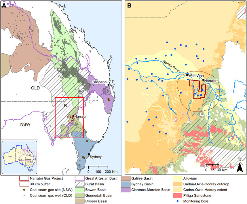
FIGURE 1. Maps showing (A) the study area within the regional extents of Surat and Gunnedah basins and the Great Artesian Basin (B).
Regional extent of the aquifer with limited monitoring data makes spatial prediction of water quality parameters difficult. Fine spatial resolution of water quality data is not available, particularly due to the fact that this is a composite unit comprising of different hydrostratigraphic units of the GAB sequence. Interpolation from available limited data can cause significant errors in prediction in such cases.
In order to adequately estimate the kriging models (described below), a sufficient number of observations are needed for each baseline water quality variable. We make the choice to limit our analysis only to baseline water quality variables where at least five unique spatial observations were available in the study region. This resulted in 41 different water quality variables from 60 different spatial locations. Primarily, these variables focus on concentrations of ions, alkalinity, total dissolved solids, pH, and other water quality indicators. The associated baseline water quality variables used are found in Table 1. The locations of the observations used are found in Figure 2. Note that sometimes only one water quality variable was observed at a spatial location.
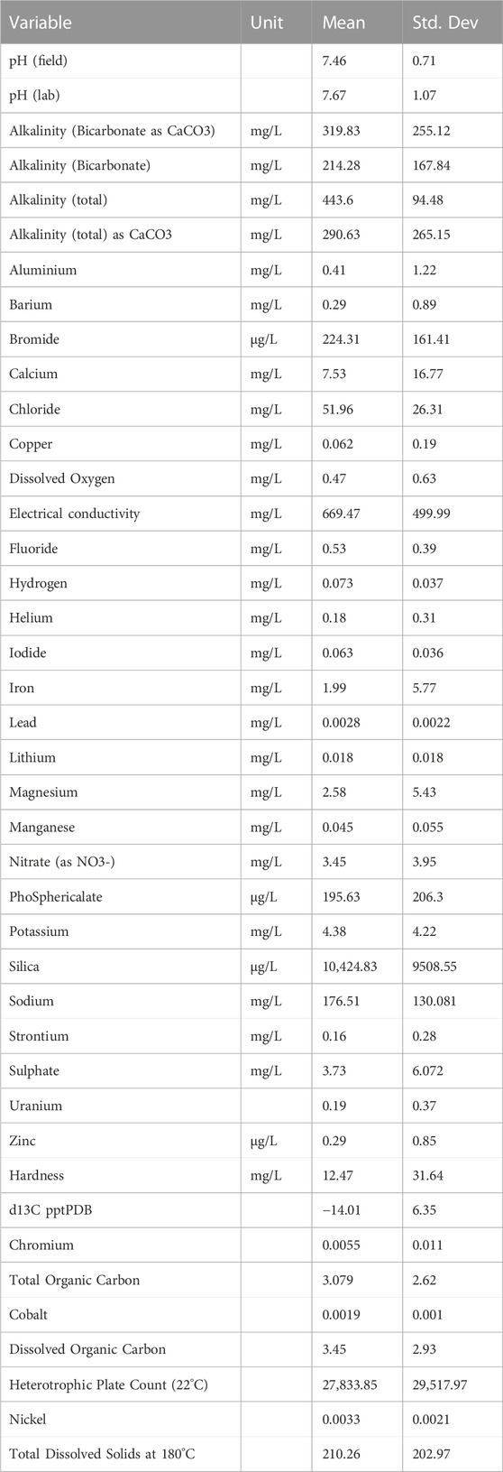
TABLE 1. Baseline water quality variables with at least 5 observations in the study region with mean and standard deviation.
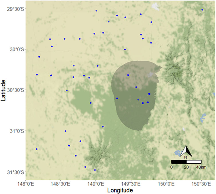
FIGURE 2. Locations with at least one water quality observation (blue) in the Pilliga Sandstone unit. The shaded region indicates the 30-km buffer region of interest.
2.2 Geostatistical kriging model
We developed individual kriging models for each of the 41 baseline water quality variables found in Table 1. Kriging models incorporate Gaussian Processes to account for the spatial variability (Cressie, 1993). The Kriging models were developed to create an optimal spatial interpolation between observations, achieved via a spatially defined mean and covariance structure used to account for spatial variability. Due to the sparse nature of our observations, and for simplicity, we make the assumption that the data are continuous and stationary across space. These assumptions are reasonable for sedimentary aquifers where significant geological structures or other features don’t cause discontinuities in groundwater flow. That is, we assume the underlying spatial processes of each water quality variable is invariant with respect to translations in space and defined at all spatial locations in the region of interest. Formally, we define the
where
where
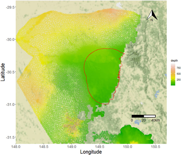
FIGURE 3. Depth to the mid-point of the Pilliga Sandstone unit used as potential covariates in kriging models. The red outline shows the 30-km buffer zone.
2.2.1 Interpolation
Importantly, we want to interpolate each water quality variable at some unknown locations
Interpolating over the area shown in Figure 2 requires decisions to be made about the resolution of each unobserved spatial location. For our purposes, we preferred as fine a spatial resolution while still allowing for reasonable computational expense for the optimization algorithm. We settled at 20,000 pixels in the 30-km buffer zone pictured in Figure 2, resulting in a 487-m resolution.
2.2.2 Covariance functions
In order to interpolate water quality variables using Eqs 3, 4, we must first determine what covariance function is appropriate for each of the
where
For each of the
2.3 Optimal monitoring design using differential evolution
In order to determine the optimal locations for monitoring that will reduce prediction uncertainty, we use the results of the 41 kriging models developed in Section 2.2. We used the Differential Evolution algorithm (Storn and Price, 1997; Mullen et al., 2011) to identify the optimal locations. Sreekanth et al. (2017) demonstrated the applicability of the algorithm for groundwater monitoring network designs.
Specifically, we seek to find the set of m borehole locations, denoted as
where
The optimization algorithm then searchers for optimal borehole locations that minimize Eq. 6. This is done by using Differential Evolution via the DEoptim package in the R statistical computing language (Mullen et al., 2011; R Core Team, 2022). For our purposes, we seek an optimization of
3 Results
We developed kriging models for each of the 41 baseline water quality indicators described in Section 2. We first do this by estimating the covariance functions from the empirical variograms for each water quality variable, considering whether we include depth as a covariate or not. This resulted in depth being included in 18 of the 41 kriging models, with a mean reduction in error of 35.5% (minimum 0.3%, maximum 99.9%). Further, the majority of the water quality variables used the Matérn covariance function, used in 27 of the kriging models, with the spherical covariance function having 7, Gaussian having 6, and only 1 for the Exponential covariance function. Table 2 shows whether depth was included, the covariance function used, and the estimates of the parameters for all 41 water quality variables.
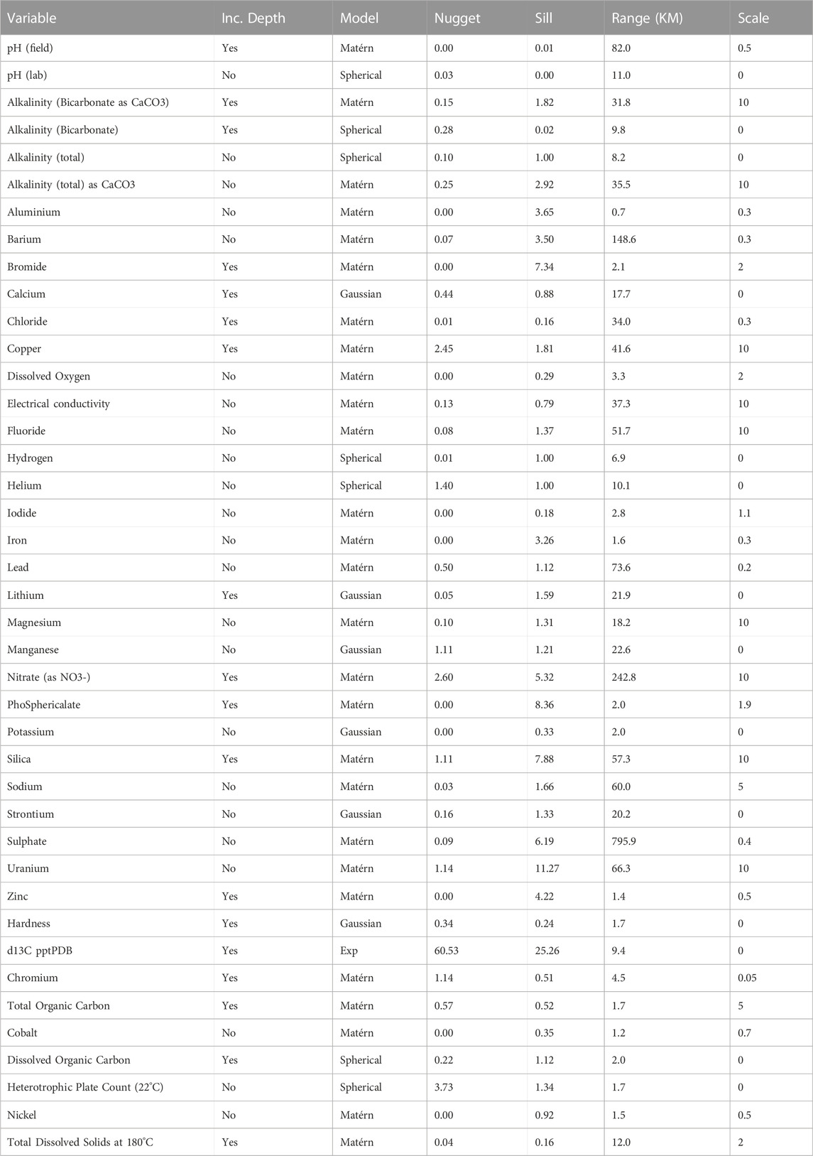
TABLE 2. Covariance function and parameter estimates and inclusion of depth as a covariate for all baseline water quality variables.
Once we determined the best kriging models, we used the Differential Evolution algorithm with the objective function described in Section 2.3 to identify 10 potential borehole locations that will reduce prediction uncertainty in baseline water quality indicators in the 30-km buffer zone. Figure 4 shows the optimal locations of these borehole locations in the 30-km buffer zone.
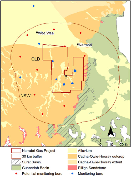
FIGURE 4. Potential new bore locations (red) for monitoring baseline water quality in the Pilliga Sandstone unit and existing bore locations with at least one water quality observation (blue).
These optimal locations reduce prediction uncertainty across all potential water quality variables. We inspect the resulting interpolation before and after establishing optimal locations of the boreholes in the buffer region. For brevity, we present 3 examples: pH field, electrical conductivity, and alkalinity as bicarbonate. The variable pH field did not have any observations in the buffer region while electrical conductivity and alkalinity as bicarbonate did. Further, pH field and alkalinity bicarbonate used depth as an added covariate while electrical conductivity did not. Figures 5–7 show the reduction in uncertainty for pH field, electrical conductivity, and alkalinity bicarbonate, respectively. All three show a general trend in reduced variance with the addition of optimal monitoring bores. It is observable that the variance is significantly reduced within the whole 30-km buffer zone even when the parameter (pH field) did not have any existing observations in this area.
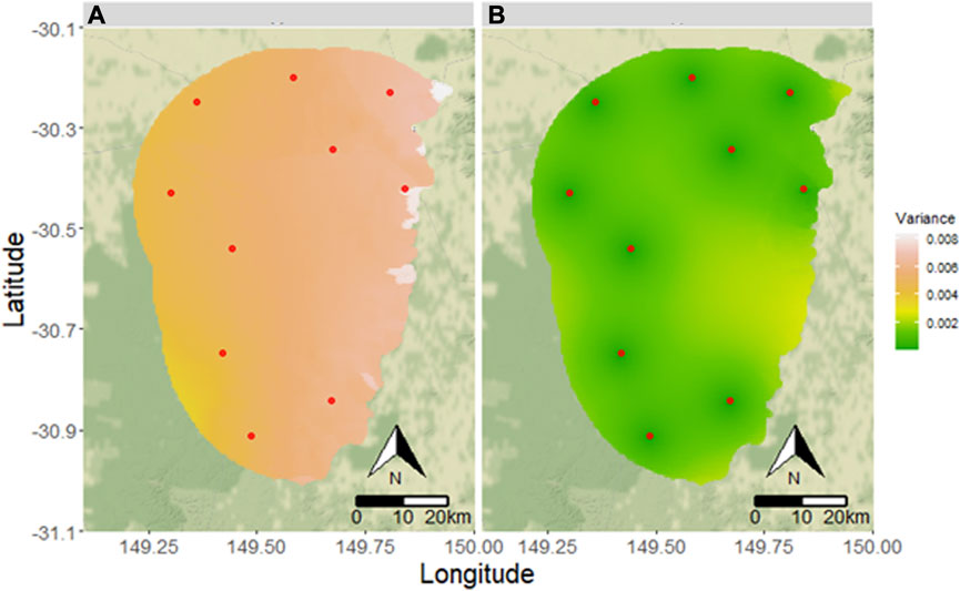
FIGURE 5. Estimated variance for pH (A) without new monitoring locations and (B) after optimization and supplementation with the new monitoring locations for “pH field” water quality variable. Red dots indicate potential new monitoring locations.
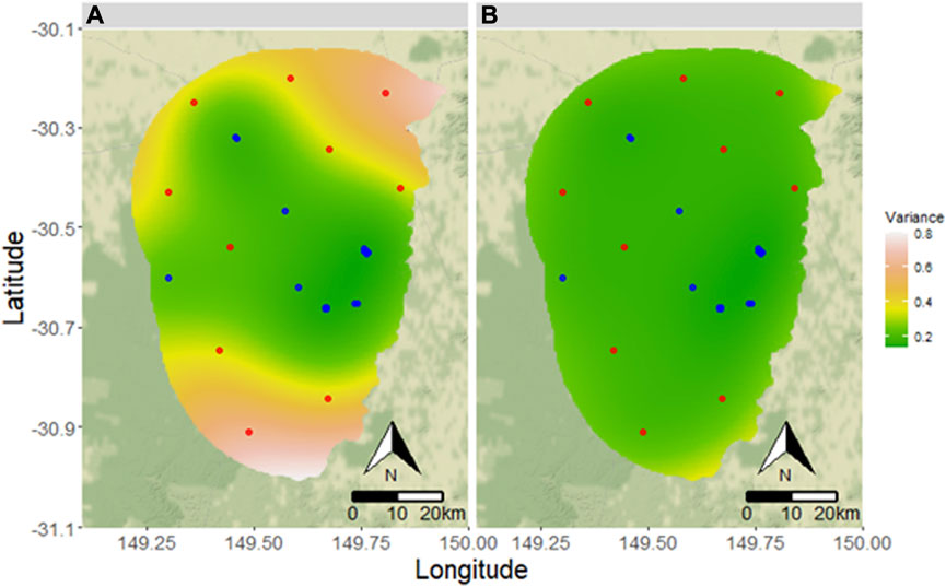
FIGURE 6. Estimated variance of electrical conductivity (A) without new monitoring locations and (B) after optimization and supplementation with the new monitoring locations for “Electrical Conductivity” water quality variable. Red dots indicate potential new monitoring locations. Blue dots indicate existing observations.
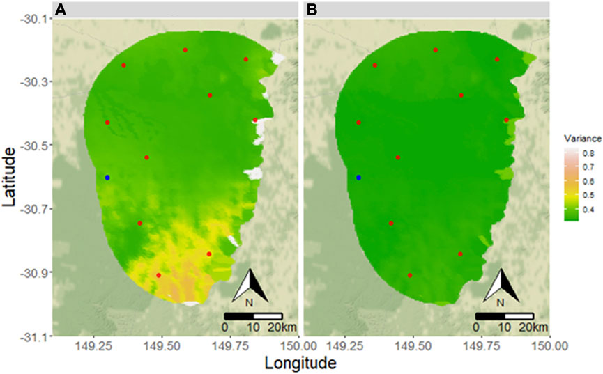
FIGURE 7. Estimated variance of bicarbonate (A) without new monitoring locations and (B) after optimization and supplementation with the new monitoring locations for “Alkalinity Bicarbonate” water quality variable. Red dots indicate potential new monitoring locations. Blue dots indicate existing observations.
Visually (Figures 5–8), our method appears to reduce prediction uncertainty for pH field, electrical conductivity, and alkalinity bicarbonate. To show that our method reduced uncertainty for all baseline water quality indicators, we present a summary of standard deviations aggregated across pixels for each variable. Specifically, we present a 95% confidence interval (in the form of 2.5th and 97.5th percentiles for the lower and upper bounds) and the median standard deviations across all interpolated pixels for the original kriging models and inclusion of the optimal borehole locations. For comparison purposes, we also include these values from choosing a random set of boreholes in the buffer region. These results are found in Table 3. As expected, the standard deviations across all water quality variables has decreased. Critically, each water quality variable had lower uncertainties when optimal locations were included compared to the random locations. While we do not compare all possible 10-borehole situations due to computational expense, our experience indicated that regardless of which combination of spatial locations we chose, the optimal borehole location produced the highest reduction in uncertainty (that is, the lowest standard deviations).
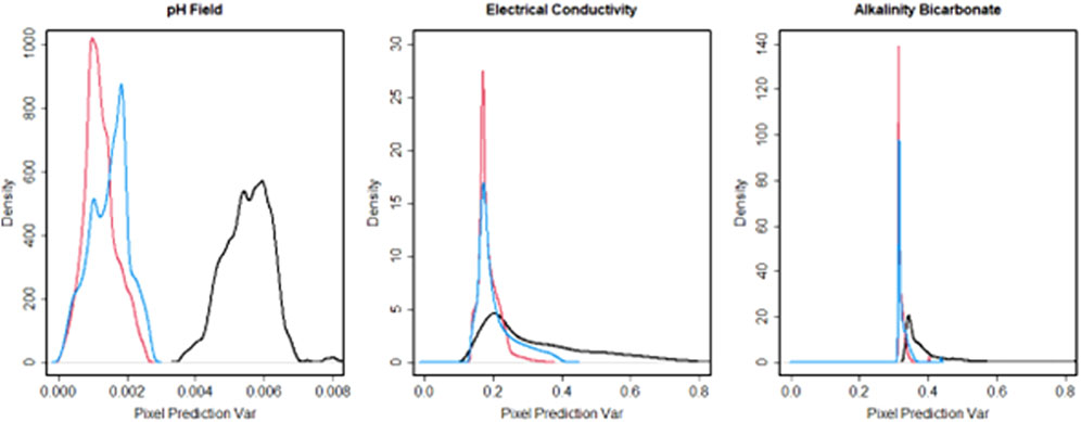
FIGURE 8. Density estimates of prediction variance across all pixels in the buffer region. Left plot shows pH field, middle shows Electrical Conductivity, and right shows Alkalinity Bicarbonate. Black lines indicate original prediction uncertainty, red shows prediction uncertainty if the optimal borehole locations were included, and blue shows a prediction uncertainty when using random borehole locations.
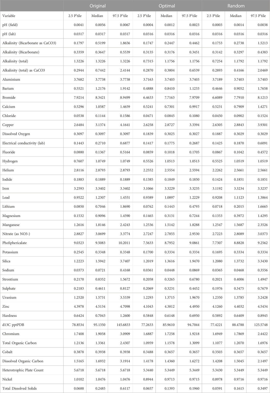
TABLE 3. Summary of standard deviations across pixels for the original kriging models, inclusion of optimal borehole locations, and inclusion of random borehole locations. The percentiles presented are 2.5th, median, and 97.5th percentiles.
It is noteworthy that there are different ways to approach the groundwater monitoring network design problem. For example, the design may include identifying the optimal number of bores required for a specific purpose as one of the design objectives. In this study, we did not consider any specific purpose of design other than minimizing the uncertainty of several water quality parameters within a chosen area. Hence, we specified the number of bores to be 10. In the practical contexts, it is often the budget that prescribe the number of bores to be drilled. However, there are contexts in which decision maker may be interested in identifying the optimal number of bores to be drilled for a specific monitoring goal. Certainly, it stands to reason that there will be diminishing returns in uncertainty reduction with increasing number of boreholes, but we believe this would be a question for another research study, given our interest in this study is showcasing a new method for determining optimal borehole locations. This would require a rule for determining how much uncertainty may be reduced for increasing boreholes and finding out when adding more provides minimal reduction in uncertainty. It is also important to note the limitations of the study that the monitoring network design approach presented in this study is based on statistical variance reduction and assumes that the parameters vary continuously in space with plausible spatial covariance structures. Physical processes that may influence abrupt changes in these water quality parameters were assumed to be absent. Indeed, a limitation of this study is the accuracy of the spatial interpolation. The methodology may not be applicable in areas or contexts in which parameters vary abruptly or randomly and lack spatial covariance.
4 Conclusion
We developed an optimization approach for designing optimal monitoring bore locations for water quality measurements and demonstrated the applicability of the method for reducing uncertainty in the spatial prediction of many water quality parameters using observations from a limited number of bores. The method makes use of multiple geostatistical Kriging models for spatial modelling of many groundwater quality parameters. The kriging models were then used in conjunction with a Differential Evolution algorithm to determine optimal monitoring locations that minimized prediction variance of all considered water quality parameters.
The method is demonstrated by applying it for designing a 10-bore monitoring network in the Pilliga Sandstone aquifer in the Namoi region of Australia. Evaluations indicate that the optimal network is able to reduce the prediction variances for all water quality parameters. The use of kriging models makes it computationally feasible to include large number of water quality parameters in the monitoring network design. Thus, the method is scalable to practical contexts where regulatory or other agencies want to optimize drilling of monitoring bores for monitoring all baseline water quality parameters (Janardhanan et al., 2019).
Data availability statement
The original contributions presented in the study are included in the article/Supplementary material, further inquiries can be directed to the corresponding author.
Author contributions
SJ developed and led the project, developed parts of the methodology and wrote parts of the paper. DWG completed the geostatistical and optimization analysis and drafted the initial version of the manuscript. DP developed parts of the methodology and contributed the analysis. DeG contributed to the analysis and prepared the maps. All authors contributed to the article and approved the submitted version.
Acknowledgments
This research was funded by the Commonwealth Scientific and Industrial Research Organisation’s (CSIRO) Gas Industry Social and Environmental Research Alliance (GISERA). GISERA is a collaboration between CSIRO, Commonwealth and state governments and industry established to undertake publicly-reported independent research. The purpose of GISERA is for CSIRO to provide quality assured scientific research and information to communities living in gas development regions focusing on social and environmental topics including: groundwater and surface water, biodiversity, land management, the marine environment, human health impacts and socio-economic impacts. The governance structure for GISERA is designed to provide for and protect research independence and transparency of research outputs.
Conflict of interest
The authors declare that the research was conducted in the absence of any commercial or financial relationships that could be construed as a potential conflict of interest.
Publisher’s note
All claims expressed in this article are solely those of the authors and do not necessarily represent those of their affiliated organizations, or those of the publisher, the editors and the reviewers. Any product that may be evaluated in this article, or claim that may be made by its manufacturer, is not guaranteed or endorsed by the publisher.
References
Ammar, K., Khalil, A., McKee, M., and Kaluarachchi, J. (2008). Bayesian deduction for redundancy detection in groundwater quality monitoring networks. Water Resour. Res. 44 (8). doi:10.1029/2006wr005616
Aryal, S. K., Northey, J., Slatter, E., Ivkovic, K., Crosbie, R., Janardhanan, S., et al. (2018). “Observations analysis, statistical analysis and interpolation for the Namoi subregion,” in Product 2.1-2.2 for the Namoi subregion from the northern inland catchments bioregional assessment (Canberra, Australia: Department of the Environment and Energy, Bureau of Meteorology, CSIRO and Geoscience Australia). http://data.bioregionalassessments.gov.au/product/NIC/NAM/2.1-2.2.
Asefa, T., Kemblowski, M., Lall, U., Urroz, G., Mckee, M., and Khalil, A. (2004). Support vectors-based groundwater head observation networks design. Water Resour. Res. 40(11). doi:10.1029/2004wr003304
Asefa, T., Kemblowski, M., Lall, U., and Urroz, G. (2005). Support vector machines for nonlinear state space reconstruction: application to the Great Salt Lake time series. Water Resour. Res. 41. W12422, doi:10.1029/2004wr003785
Ayvaz, M. T., and Elçi, A. (2018). Identification of the optimum groundwater quality monitoring network using a genetic algorithm based optimization approach. J. Hydrology 563, 1078–1091. doi:10.1016/j.jhydrol.2018.06.006
Bode, F., Ferré, T. P. A., Zigelli, N., Emmert, M., and Nowak, W. (2018). Reconnecting stochastic methods with HydrogeologicalApplications: A utilitarian uncertainty analysis and RiskAssessment approach for the design of OptimalMonitoring networks. Water Resour. Res. 54, 2270–2287. doi:10.1002/2017WR020919
Chadalavada, S., and Datta, B. (2008). Dynamic optimal monitoring network design for transient transport of pollutants in groundwater aquifers. Water Resour. Manag. 22, 651–670. doi:10.1007/s11269-007-9184-x
Cressie, N. (1993). Aggregation in geostatistical problems. Amsterdam, Netherlands: Springer, 25–36.
Cressie, N., and Wikle, C. K. (2011). Statistics for spatio-temporal data. Wiley & Sons. Hoboken, NJ, USA.
Datta, B., and Dhiman, S. D. (1996). Chance-constrained optimal monitoring network design for pollutants in ground water. J. Water Resour. Plan. Manag. 122 (3), 180–188. doi:10.1061/(asce)0733-9496(1996)122:3(180)
Dhar, A., and Datta, B. (2007). Multiobjective design of dynamic monitoring networks for detection of groundwater pollution. J. water Resour. Plan. Manag. 133 (4), 329–338. doi:10.1061/(asce)0733-9496(2007)133:4(329)
Dokou, Z., and Pinder, G. F. (2009). Optimal search strategy for the definition of a DNAPL source. J. Hydrology 376 (3-4), 542–556. doi:10.1016/j.jhydrol.2009.07.062
Fan, Y., Lu, W., Miao, T., Li, J., and Lin, J. (2020). Multiobjective optimization of the groundwater exploitation layout in coastal areas based on multiple surrogate models. Environ. Sci. Pollut. Res. 27 (16), 19561–19576. doi:10.1007/s11356-020-08367-2
Herrera, G. S., and Pinder, G. F. (2005). Space-time optimization of groundwater quality sampling networks. Water Resour. Res. 41 (12). doi:10.1029/2004wr003626
Hosseini, M., and Kerachian, R. (2017). A data fusion-based methodology for optimal redesign of groundwater monitoring networks. J. Hydrology 552, 267–282. doi:10.1016/j.jhydrol.2017.06.046
Hudak, P. F., and Loaiciga, H. A. (1992). A location modeling approach for groundwater monitoring network augmentation. Water Resour. Res. 28 (3), 643–649. doi:10.1029/91wr02851
Janardhanan, S., Gladish, D., Gonzalez, D., Pagendam, D., Pickett, T., and Cui, T. (2019). Optimal design and prediction-independent verification of groundwater monitoring network. Water 12 (1), 123. doi:10.3390/w12010123
Kollat, J. B., and Reed, P. M. (2007). A computational scaling analysis of multiobjective evolutionary algorithms in long-term groundwater monitoring applications. Adv. Water Resour. 30 (3), 408–419. doi:10.1016/j.advwatres.2006.05.009
Kollat, J. B., and Reed, P. M. (2006). Comparing state-of-the-art evolutionary multi-objective algorithms for long-term groundwater monitoring design. Adv. Water Resour. 29 (6), 792–807. doi:10.1016/j.advwatres.2005.07.010
Kollat, J. B., Reed, P. M., and Kasprzyk, J. R. (2008). A new epsilon-dominance hierarchical Bayesian optimization algorithm for large multiobjective monitoring network design problems. Adv. Water Resour. 31 (5), 828–845. doi:10.1016/j.advwatres.2008.01.017
Kollat, J. B., Reed, P. M., and Maxwell, R. M. (2011). Many-objective groundwater monitoring network design using bias-aware ensemble Kalman filtering, evolutionary optimization, and visual analytics. Water Resour. Res. 47 (2). doi:10.1029/2010wr009194
Loaiciga, H. A. (1989). An optimization approach for groundwater quality monitoring network design. Water Resour. Res. 25 (8), 1771–1782. doi:10.1029/wr025i008p01771
Luo, Q., Wu, J., Yang, Y., Qian, J., and Wu, J. (2016). Multi-objective optimization of long-term groundwater monitoring network design using a probabilistic Pareto genetic algorithm under uncertainty. J. Hydrology 534, 352–363. doi:10.1016/j.jhydrol.2016.01.009
Mahar, P. S., and Datta, B. (1997). Optimal monitoring network and ground-water–pollution source identification. J. water Resour. Plan. Manag. 123 (4), 199–207. doi:10.1061/(asce)0733-9496(1997)123:4(199)
Massmann, J., and Freeze, R. A. (1987). Groundwater contamination from waste management sites: the interaction between risk-based engineering design and regulatory policy: 1. methodology. Water Resour. Res. 23 (2), 351–367. doi:10.1029/wr023i002p00351
McKinney, D. C., and Loucks, D. P. (1992). Network design for predicting groundwater contamination. water Resour. Res. 28 (1), 133–147. doi:10.1029/91wr02397
Meyer, P. D., and Brill, E. D. (1988). A method for locating wells in a groundwater monitoring network under conditions of uncertainty. Water Resour. Res. 24 (8), 1277–1282. doi:10.1029/wr024i008p01277
Mirzaie-Nodoushan, F., Bozorg-Haddad, O., and Loáiciga, H. A. (2017). Optimal design of groundwater-level monitoring networks. J. Hydroinformatics 19 (6), 920–929. doi:10.2166/hydro.2017.044
Montas, H. J., Mohtar, R. H., Hassan, A. E., and AlKhal, F. A. (2000). Heuristic space–time design of monitoring wells for contaminant plume characterization in stochastic flow fields. J. Contam. Hydrology 43 (3-4), 271–301. doi:10.1016/s0169-7722(99)00108-4
Mullen, K. M., Ardia, D., Gil, D., Windover, D., and Cline, J. (2011). DEoptim: an r package for global optimization by differential evolution. J. Stat. Softw. 40 (6), 1–26. doi:10.18637/jss.v040.i06
Nunes, L. M., Cunha, M. C., and Ribeiro, L. (2004). Groundwater monitoring network optimization with redundancy reduction. J. Water Resour. Plan. Manag. 130 (1), 33–43. doi:10.1061/(asce)0733-9496(2004)130:1(33)
R Core Team (2022). R: A language and environment for statistical computing. R Foundation for Statistical. Ames, IA, USA.
Reed (2000). Computing, Springer, Vienna, Austria. URL https://www.R-project.org/.Reed.
Reed, P., Kollat, J. B., and Devireddy, V. K. (2007). Using interactive archives in evolutionary multiobjective optimization: A case study for long-term groundwater monitoring design. Environ. Model. Softw. 22 (5), 683–692. doi:10.1016/j.envsoft.2005.12.021
Reed, P., Minsker, B. S., and Goldberg, D. E. (2003). Simplifying multiobjective optimization: an automated design methodology for the nondominated sorted genetic algorithm-ii. Water Resour. Res. 39 (7). doi:10.1029/2002wr001483
Reed, P. M., and Minsker, B. S. (2004). Striking the balance: long-term groundwater monitoring design for conflicting objectives. J. Water Resour. Plan. Manag. 130 (2), 140–149. doi:10.1061/(asce)0733-9496(2004)130:2(140)
Rizzo, D. M., Dougherty, D. E., and Yu, M. (2000). “An adaptive long-term monitoring and operations system (aLTMOsTM) for optimization in environmental management,” In Building partnerships, ASCE 2000 Joint Conf. on Water Resources Engineering and Water Resources Planning and Management, ASCE, Reston, VA, 1–10. doi:10.1061/40517(2000)113
Ruiz-Cárdenas, R., Ferreira, M. A., and Schmidt, A. M. (2010). Stochastic search algorithms for optimal design of monitoring networks. Environmetrics official J. Int. Environmetrics Soc. 21 (1), 102–112. doi:10.1002/env.989
Song, J., Yang, Y., Chen, G., Sun, X., Jin, L., Wu, J., et al. (2019). Surrogate assisted multi-objective robust optimization for groundwater monitoring network design. J. Hydrology 577, 123994. doi:10.1016/j.jhydrol.2019.123994
Sreekanth, J., Crosbie, R., Pickett, T., Cui, T., Peeters, L., Slatter, E., et al. (2017). “Groundwater numerical modelling for the Namoi subregion,” in Product 2.6.2 for the Namoi subregion from the northern inland catchments bioregional assessment (Canberra, Australia: Department of the Environment and Energy, Bureau of Meteorology, CSIRO and Geoscience Australia).
Sreekanth, J., Gladish, D., Gonzalez, D., Pagendam, D., Pickett, T., and Cui, T. (2018). CSG-Induced groundwater impacts in the Pilliga region: Prediction uncertainty, data-worth and optimal monitoring strategies. Canberra, Australia: Commonwealth Scientific and Industrial Research Organisation.
Storn, R., and Price, K. (1997). Differential evolution—a simple and efficient heuristic for global optimization over continuous spaces. J. Glob. Optim. 11 (4), 341–359. doi:10.1023/A:1008202821328
Wagner, B. J. (1995). Recent advances in simulation-optimization groundwater management modeling. Rev. Geophys. 33 (2), 1021–1028. doi:10.1029/95rg00394
Wu, J., Zheng, C., and Chien, C. C. (2005). Cost-effective sampling network design for contaminant plume monitoring under general hydrogeological conditions. J. Contam. Hydrology 77 (1-2), 41–65. doi:10.1016/j.jconhyd.2004.11.006
Wu, J., Zheng, C., Chien, C. C., and Zheng, L. (2006). A comparative study of Monte Carlo simple genetic algorithm and noisy genetic algorithm for cost-effective sampling network design under uncertainty. Adv. Water Resour. 29 (6), 899–911. doi:10.1016/j.advwatres.2005.08.005
Keywords: groundwater monitoring, network design, optimization, differential evolution, spatial statistics
Citation: Gladish DW, Pagendam DE, Janardhanan S and Gonzalez D (2023) Geostatistical based optimization of groundwater monitoring well network design. Front. Earth Sci. 11:1188316. doi: 10.3389/feart.2023.1188316
Received: 17 March 2023; Accepted: 22 August 2023;
Published: 06 September 2023.
Edited by:
Debabrata Sahoo, Clemson University, United StatesReviewed by:
Dillip Barik, Vellore Institute of Technology, IndiaDebasmita Misra, University of Alaska Fairbanks, United States
Ty Ferre, University of Arizona, United States
Copyright © 2023 Gladish, Pagendam, Janardhanan and Gonzalez. This is an open-access article distributed under the terms of the Creative Commons Attribution License (CC BY). The use, distribution or reproduction in other forums is permitted, provided the original author(s) and the copyright owner(s) are credited and that the original publication in this journal is cited, in accordance with accepted academic practice. No use, distribution or reproduction is permitted which does not comply with these terms.
*Correspondence: Sreekanth Janardhanan, c3JlZWthbnRoLmphbmFyZGhhbmFuQGNzaXJvLmF1
†ORCID ID: Daniel E. Pagendam, orcid.org/0000-0002-8347-4767