Optimal parameters of random forest for land cover classification with suitable data type and dataset on Google Earth Engine

Exact land cover (LC) map is essential information for understanding the development of human societies and studying the impacts of climate and environmental change. To fulfill this requirement, an optimal parameter of Random Forest (RF) for LC classification with suitable data type and dataset on Google Earth Engine (GEE) was investigated. The research objectives were 1) to examine optimum parameters of RF for LC classification at local scale 2) to classify LC data and assess accuracy in model area (Hefei City), 3) to identify a suitable data type and dataset for LC classification and 4) to validate optimum parameters of RF for LC classification with a suitable data type and dataset in test area (Nanjing City). This study suggests that the suitable data types for LC classification were Sentinel-2 data with auxiliary data. Meanwhile, the suitable dataset for LC classification was monthly and seasonal medians of Sentinel-2, elevation, and nighttime light data. The appropriate values of the number of trees, the variable per split, and the bag fraction for RF were 800, 22, and 0.9, respectively. The overall accuracy (OA) and Kappa index of LC in model area (Hefei City) with suitable dataset was 93.17% and 0.9102. In the meantime, the OA and Kappa index of LC in test area (Nanjing City) was 92.38% and 0.8914. Thus, the developed research methodology can be applied to update LC map where LC changes quickly occur.

1 Introduction

Detailed, timely and accurate land cover (LC) can help people understand the relationship between the development of human societies and climate and environmental change (Turner et al., 2007; Song et al., 2018; Liu et al., 2020b). LC classification and mapping are considered to be the key technologies to obtain surface information at various scales (Feddema et al., 2005), which is critical for understanding the impact of LC changes on agricultural production, ecotourism, carbon sequestration, water quality, runoff, and species conservation. In recent years, more and more fields require LC maps with higher temporal and spatial resolution, and more and more government departments and institutions need LC maps as the basis for decision-making, planning, and budgeting. However, due to surface heterogeneity and spectral confusion, accurate LC classification and mapping still face many challenges, especially in utilizing time-series satellite data.

The Landsat images have been shared data source for LC mapping and monitoring in the past 50 years (Hansen and Loveland, 2012; Gómez et al., 2016). The Sentinel-2 (S2) satellite provides higher spatial and spectral resolution data than Landsat and opens up new opportunities for LC classification (Pirotti et al., 2016; Forkuor et al., 2018). Recent studies have demonstrated that S2 data can classify LC from a single date image (Clark, 2017; Mongus and Žalik, 2018). However, a single scene of such data cannot effectively monitor dynamic changes to distinguish spectrally similar LC classes. Time-series images often yield better performance than single-temporal images do (Sothe et al., 2017). S2 is superior to Landsat in terms of spatial resolution, time resolution and spectral bands, and it can provide rich phenological information, spatial information and spectral information, making it an increasingly important data source for LC classification.

Nevertheless, the availability of optical data becomes limited and difficult with the occurrence of frequent cloud cover when more than one cloud-free observation per month in time-series images is required for LC classification (Ju and Roy, 2008). The synthetic aperture radar (SAR) data have been increasingly utilized recently as they do not rely on sunlight and are not influenced by cloud and fog (DeFries, 2008; Freitas et al., 2008; Zeng et al., 2020). By exploiting different physical principles, the optical and radar data deliver complementary information, providing higher accuracy for LC classification than a single data source do (Erasmi and Twele, 2009; Stefanski et al., 2014; Joshi et al., 2016). With the free open-access policy of the ESA Sentinel satellite constellation, both multi-sensor and multi-temporal LC mapping have become even more attractive (Drusch et al., 2012; Torres et al., 2012). Some studies have used the multi-sensor method of Sentinel-1 (S1) and S2 data for LC classification and mapping (Pesaresi et al., 2016; Ban et al., 2017; Chatziantoniou et al., 2017; Clerici et al., 2017).

LC is usually affected by natural conditions and human activities. Elevation data can intuitively reflect the natural conditions of a region, while nighttime light images provide unique footprints of human activities and settlements. More and more scholars have begun to add night light data and elevation data to the classification of LC, and discuss their importance in the classification of LC. For example, Tang et al. (2020) use JL1-3B high-resolution nighttime light imagery and Sentinel-2 time series imagery fusion for impervious surface area mapping. Goldblatt et al. (2018) classify the urban LC with fusion approach utilizing nighttime light data and Landsat imagery. Liu et al. (2020a) classified the Landsat data for the Gannan Prefecture and the results showed that the topographic features contributed the most, followed by the spectral indices and bands. Phan et al. (2020) used Landsat 8 data to classify the LC in Mongolia, and the results showed that elevation was the most important feature.

In recent years, deep learning (DL) and machine learning (ML) have gained increasing attention, and their uses are constantly increasing in LC classification. DL is often confusing with ML, but it should be noted that DL is a subset of ML, and both belong to the category of artificial intelligence (AI) (Chen et al., 2019; Klaiber, 2021). The commonly used ML algorithms include linear regression, logistic regression, naïve bayes (NB), support vector machines (SVM), decision tree, Bayesian learning, K nearest neighbor (KNN), neural networks (NN) and random forest (RF) (Ray, 2019). DL algorithms are the upgraded version of artificial neural networks, and commonly used DL algorithms include deep Boltzmann machine (DBM), deep belief network (DBN), convolutional neural network (CNN), graph convolutional network (GCN), recurrent neural networks (RNN), and recursive neural networks (RvNN) (Shrestha and Mahmood, 2019; Hong et al., 2021a; Hong et al., 2021b; Wu et al., 2022). In the field of LC classification, these state-of-the-art (SOTA) classification methods mentioned above and their improved algorithms have been widely adopted in various research topics. Lin et al. (2018) extract the LC types of Weihai from 1985–2015 using SVM classification method with Landsat MSS/TM/OLI images. Thanh Noi and Kappas (2018) compare RF, KNN, and SVM for LC classification using Sentinel-2 in Red River Delta. Sun et al. (2019) build a long short-term memory (LSTM) RNN model for LC classification in North Dakota with time series Landsat. Hong et al. (2021a) develop a new minibatch GCN for hyperspectral image classification, which allows to train large-scale GCNs in a minibatch fashion.

The RF (Breiman, 2001), which is one of ML classifiers and developed based on decision tree, became one of the favorite and most promising LC classifiers due to its relatively stable and robust classification accuracy and effectiveness in handling large and high-dimensional datasets, and it has been widely used in multi-temporal and multi-sensor images classification (Gislason et al., 2006; Rodriguez-Galiano et al., 2012; Pelletier et al., 2016; Ghorbanian et al., 2020; Phan et al., 2020; Ghorbanian et al., 2021). Bourgoin et al. (Bourgoin et al., 2020) used the RF algorithm for LC classification based on Landsat and S2 data and reported overall accuracy (OA) and Kappa index of 0.81 and 0.87, respectively.

Recently, the explosive growth in data volume, including multi-temporal and multi-sensor datasets that are effective in LC information extraction, has led to problems of time consumption with low efficient processing using personal or workstation computers. The Google Earth Engine (GEE) can easily get access to multi-sensor and multi-temporal images and it provides high-performance operation without downloading these data to a local machine (Gorelick et al., 2017; Kumar and Mutanga, 2018; Mutanga and Kumar, 2019; Amani et al., 2020; Tamiminia et al., 2020). Furthermore, the temporal aggregation method, such as the median, in the GEE significantly reduces cloud interference, resolves the problems of unavailable satellite data for specific periods. In addition, the availability of powerful classification models, such as RF (Shelestov et al., 2017), makes the GEE a widely used remote-sensing tool for LC research. Some studies have used the RF algorithm to classify LC on the GEE platform (Azzari and Lobell, 2017; Ghorbanian et al., 2020; Phan et al., 2020; Zhang et al., 2020; Yang et al., 2021).

Meanwhile, LC datasets at regional and global scales, including FROM-GLC30 (Gong et al., 2013), FROM-GLC10 (Gong et al., 2019), GlobeLand30 (Chen et al., 2015), GLC_FCS30 (Zhang et al., 2021), ESA WorldCover (Zanaga et al., 2021), and ESRI Land Cover (Krishna et al., 2021) are available for public uses. In this study, the LC dataset in 2020 was used as reference data to extract training and validating areas and examine optimal parameters of RF for LC classification at a local scale under the GEE platform with S1 and S2 satellites in the model area. Then, the derived optimal parameters of RF were applied to classify LC type in the test area with the suitable dataset for validation.

Our specific research objectives were 1) to examine optimum parameters of RF for LC classification at local scale 2) to classify LC data and assess accuracy in model area (Hefei City), 3) to identify a suitable data type and dataset for LC classification and 4) to validate optimum parameters of RF for LC classification with a suitable data type and dataset in test area (Nanjing City). The proposed method can reduce the cost for updating LC map at local scale.

2 Materials and methods

2.1 Study area

Hefei City and Nanjing City were selected as the model and test areas respectively. Hefei City, with a population of more than 8 million, is the capital and the largest city in Anhui Province, China. It was chosen to examine an optimal parameter of RF and to identify a suitable data type and dataset for LC classification (Figure 1A). At the same time, Nanjing City, with a population of more than 8.5 million, is a sub-provincial city and the capital city in Jiangsu Province, China. It was selected to validate the optimal parameters of RF for LC classification under GEE with suitable datatype and dataset (Figure 1B).

FIGURE 1

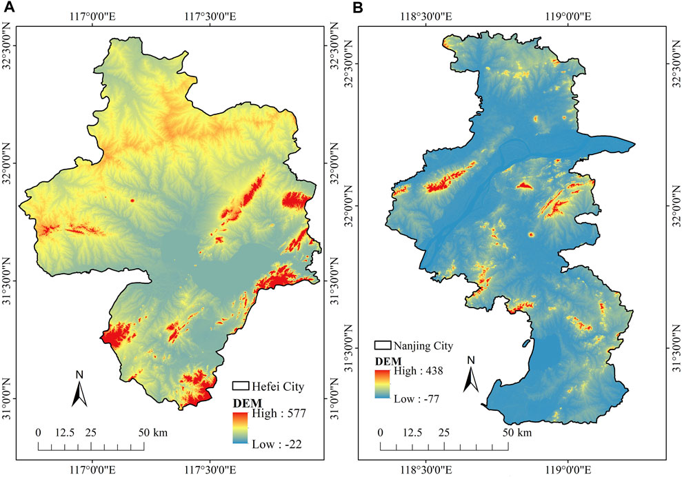
FIGURE 1. Location of the study area: (A) model area (Hefei City), and (B) test area (Nanjing City).

2.2 Data

The data used in this study were categorized into three groups: 1) Sentinel satellite data, 2) auxiliary data, and 3) LC data. Brief information on each data group is summarized below.

2.2.1 Sentinel satellite data

Both S1 and S2 satellites were launched by European Space Agency (ESA).

(1) S1 data (ESA, 2023b). The S1 ground range detected (GRD) products were delivered with polarizations of the vertical transmit vertical receive (VV) and the vertical transmit horizontal receive (VH). The S1 can provide continuous all-weather, high spatial (10 m), and improved temporal resolution images at C-band unaffected by clouds, to support land monitoring (Cremer et al., 2020).

(2) S2 data (ESA, 2023c). The S2 multi-spectral instrument (MSI) sensor provides high spatial (10 m) and multi-spectral images over the global surface, with unprecedented potential in LC monitoring and mapping (Drusch et al., 2012; Spoto et al., 2012; Zheng et al., 2017).

In this study, S1 GRD and S2 MSI products acquired in 2020 were the primary data input for LC classification.

2.2.2 Auxiliary data

(1) Elevation (NASA, 2023). The 30 m spatial resolution elevations over the study area were extracted from the Shuttle Radar Topography Mission (SRTM) data (Su et al., 2021). It is helpful to distinguish various LC types if we adopt the combination of satellite images and physiography variables (Phan et al., 2020).

(2) Nighttime light products (EOG, 2023). Obtained from the NPP-VIIRS day/night band (DNB), the 464 m spatial resolution nighttime light products were used to distinguish between artificial surfaces and bare ground (Miller et al., 2013).

2.2.3 LC data

(1) ESA WorldCover (ESA, 2023a). It is a global LC product with 10 m spatial resolution published by the ESA WorldCover team based on S1 and S2 data, which consists of 11 LC classes (Zanaga et al., 2021).

(2) ESRI Land Cover (ESRI, 2023). It is also a global LC product with 10 m spatial resolution produced by ESRI Impact Observatory through S2 image, which consists of 10 LC classes (Krishna et al., 2021).

The common areas of LC type of ESA WorldCover and ESRI Land Cover products are used to select training and validation samples in this study.

2.3 Methods

The research methodology consisted of 7 steps: 1) preprocessing of Sentinel satellite data, 2) feature extraction and dataset preparation, 3) selection of training and validation samples, 4) optimal parameters identification of RF, 5) LC classification and accuracy assessment in model area, 6) suitable datatype and dataset identification for LC classification, and 7) LC classification and accuracy assessment in test area. The workflow is displayed in Figure 2. Details are described in the following sections.

FIGURE 2

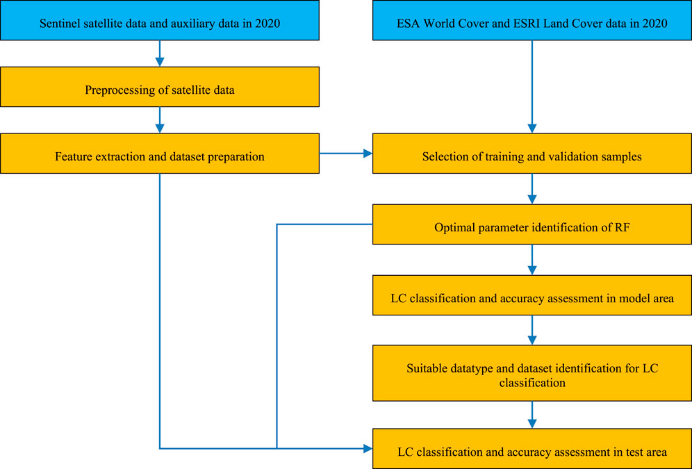
FIGURE 2. Workflow of research methodology.

2.3.1 Preprocessing of sentinel satellite data

There are two steps for preprocessing of Sentinel satellite data.

(1) Data selection, cloud pixels masking, and topographic correction for S2

Unlike S1 data, which is not affected by the cloud, scenes covered by cloud are typical in S2 data, so S2 data must be pre-processed to minimize the impact of cloud coverage. Only S2 scenes with a cloud coverage percentage of less than 85% were selected and used in subsequent steps according to the mask information of QA60 in the S2 image collection, while the S2 scenes with a cloud coverage percentage of more than 85% were removed. Then, the cloud coverage pixels in the selected S2 scene were identified and masked based on the QA60 band information, and these cloud coverage pixels did not participate in subsequent processing. Moreover, topographic correction was performed (Soenen et al., 2005) to compensate for the solar irradiance, thereby minimizing terrain-induced reflectance changes. This work was implemented by executing open-source code on GEE (https://mygeoblog.com/2018/07/27/sentinel-2-terrain-correction/). Finally, all data used in this study will be clipped to the scope of the study area to improve computational efficiency.

(2) Monthly/Seasonal median calculation for S1 and S2

To minimize the influence of holes in the image caused by the masked cloud cover pixels in the S2 scene in the previous step, and to reduce the amount of data to improve the speed of classification, the median calculation was performed. The monthly median for 12 months and seasonal median for four seasons were calculated by time aggregation for both S1 and S2 data (Luo et al., 2021; Shetty et al., 2021; Masroor et al., 2022).

2.3.2 Feature extraction and dataset preparation

For S1 data, each monthly/seasonal median included VV and VH polarizations, and the ratio between VH and VV were extracted.

For S2 data, spectral bands (Blue, Green, Red, Red Edge 1, Red Edge 2, Red Edge 3, NIR, Red Edge 4, SWIR 1, and SWIR 2) were extracted. Additionally, three significant indices for representative vegetation, urban and built-up and wetness features: normalized difference vegetation index (NDVI) (Tucker, 1979), normalized difference built index (NDBI) (Zha et al., 2003), and normalized difference water index (NDWI) (Gao, 1996) were calculated using the following equations.

$NDVI=\frac{{\rho }_{NIR}-{\rho }_{RED}}{{{\rho }_{NIR}+\rho }_{RED}}(1)$

$NDBI=\frac{{\rho }_{SWIR2}-{\rho }_{NIR}}{{{\rho }_{SWIR2}+\rho }_{NIR}}(2)$

$NDWI=\frac{{\rho }_{NIR}-{\rho }_{SWIR1}}{{{\rho }_{NIR}+\rho }_{SWIR1}}(3)$

Where ${\rho }_{RED}$, ${\rho }_{NIR}$, ${\rho }_{SWIR2}$, and ${\rho }_{SWIR1}$ are Band 4, Band 8, Band 12, and Band 11 of S2 satellite.

For auxiliary data, nighttime light data from the NPP-VIIRS DNB and elevation data from the SRTM, were added to the S1 and S2 data.

Finally, eighteen datasets were designed to examine an optimal parameter of RF and suitable data type and dataset for LC classification (Table 1). According to the data type, the datasets were categorized into six groups: S1 data (D1–D3), S1 and auxiliary data (D4–D6), S2 data (D7–D9), S2 and auxiliary data (D10–D12), S1 and S2 data (D13–D15), and S1, S2, and auxiliary data (D16–D18).

TABLE 1

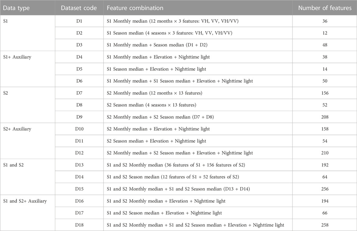
TABLE 1. Combination of features in 18 datasets for classifying LC data.

2.3.3 Selection of training and validation samples

In this study, samples were selected from the area with consistent LC attributes of ESA WorldCover and ESRI Land Cover data in 2020. In practice, the LC map from ESA WorldCover and the LC map from ESRI Land Cover were compared to find pixels with the same LC attributes, which are potential samples. Then, a stratified proportional random sampling method was used to reselect the samples from the potential samples, which could avoid the final samples from being too concentrated in a certain area or a certain LC type. As a result, a total of 5,000 samples were obtained in the model area (Hefei City), and 70% of the training samples and 30% of the validation samples were divided by using the “randomColumn” function on the GEE platform.

2.3.4 Optimal parameter of RF identification for LC classification

The operation of the RF algorithm on the GEE platform requires providing six parameters. In this study, the number of trees (NT) from 100 to 1,000 at 100-tree intervals, the variables per split (VPS) from 1 to 30 at 1-variable intervals, and the bag fraction (BF) from 0.1 to 1 at 0.1 fraction intervals were examined to identify optimal parameters of RF for LC classification. As a result, a total of 3,000 combinations (NT = 10, VPS = 30, and BF = 10) were generated and evaluated. To find suitable parameter values, the RF classifier was executed 3,000 times for each dataset (D1 to D18). Then, optimal values of three primary parameters: NT, VPS, and BF, were selected based on the small out-of-bag (OOB) error. Meanwhile, the other three parameters, maximum nodes, minimum leaf population, and seed were set up using the default values with values of null, 1, and 0, respectively.

2.3.5 LC classification and accuracy assessment in model area

This study applied the RF algorithm with optimum parameters on the GEE platform to classify six LC types: urban and built-up land, cropland, forest land, grassland, water bodies, and bare land in model area. Urban and built-up land comprises rural and urban areas, commercial and industrial areas, transportation, utilities, and infrastructures. Cropland consists of crops, orchards, tea gardens, and vegetable fields. Forest land includes natural and man-made forests. Grassland encompasses natural grass and artificial grassland. Water bodies consists of rivers, streams, ponds, and lakes. Bare land includes abandoned fields, exposed rock or soil, and open land. The expected LC types in this study were considered on the basis of the regional characteristics of Hefei City and the existing LC products. The LC classification was performed by “ee.smileRandomForest” function in the GEE.

In practices, the OA, Kappa index, producer’s accuracy (PA), and user’s accuracy (UA) calculated using “confusionMatrix.accuracy,” “ConfusionMatrix.kappa,” “confusionMatrix.producersAccuracy,” and “confusionMatrix.consumersAccuracy” functions through GEE platform, respectively, were used for the accuracy assessment (Huang et al., 2017; Lyons et al., 2018). Then, 18 groups of the OA, Kappa index, PA, and UA corresponding to 18 datasets were obtained after executing RF classifier.

2.3.6 Suitable datatype and dataset identification for LC classification

In this step, the appropriate datasets for LC classification were selected by comparing the OA and Kappa index values. Average values of OA and Kappa index by datatype, as categorized into six groups in Table 1, were applied to identify an appropriate datatype for LC classification using RF under GEE platform. Meanwhile, Kappa index values with a thresholding value of 0.8 were compared among 18 datasets to identify the suitable dataset for LC classification using RF under GEE platform.

Moreover, pairwise Z-test among top three datasets providing the highest Kappa values was applied to identify significant difference value as suggested by (Congalton and Green, 2009) as below.

$Z=\frac{\left|\widehat{K_1}-\widehat{K_2}\right|}{\sqrt{\widehat{var}\widehat{\left(K_1\right)}+\widehat{var}\widehat{\left(K_2\right)}}}(4)$

Where Z is standard normal distribution, $\widehat{K_1}$, and $\widehat{K_2}$ are Kappa indices of the first and the second dataset, and $\widehat{var}\widehat{\left(K_1\right)}$ and $\widehat{var}\widehat{\left(K_2\right)}$ are variances of Kappa indices of the first and the second dataset. The variance of Kappa index was calculated through Eq. 5.

$\widehat{var}\widehat{\left(K\right)}=\frac{1}{n}\left\{\frac{{\theta }_1\left(1-{\theta }_1\right)}{{\left(1-{\theta }_2\right)}^2}+\frac{2\left(1-{\theta }_1\right)\left(2{\theta }_1{\theta }_2-{\theta }_3\right)}{{\left(1-{\theta }_2\right)}^3}+\frac{{\left(1-{\theta }_1\right)}^2\left({\theta }_4-4{{\theta }_2}^2\right)}{{\left(1-{\theta }_2\right)}^4}\right\}(5)$

where ${\theta }_1=\frac{1}{n}{\displaystyle \sum _{i=1}^k}{n}_{ii}$,

${\theta }_2=\frac{1}{n^2}{\displaystyle \sum _{i=1}^k}{n}_{i+}{n}_{+i},$

${\theta }_3=\frac{1}{n^2}{\displaystyle \sum _{i=1}^k}{n}_{ii}\left(n_{i+}+n_{+i}\right),\text{and}$

${\theta }_4=\frac{1}{n^3}{\displaystyle \sum _{i=1}^k}{\displaystyle \sum _{j=1}^k}{n}_{ij}{\left({n_{j+}+n}_{+i}\right)}^2$

In principle, given the null hypothesis and the alternative, null hypothesis is rejected if Z ≥ Zα/2 (Congalton and Green, 2009).

2.3.7 LC classification and accuracy assessment in test area

A suitable datatype for LC classification in the model area (Hefei City) was firstly prepared for test area (Nanjing City). Then, the prepared suitable datatype was used to classify LC type with an optimal parameter of RF as identified in the Step 2.3.4. The classified LC map was assessed its thematic accuracy. The thematic accuracy information of Hefei City and Nanjing City was compared to validate LC classification using RF under GEE platform.

3 Results

3.1 Optimal parameters of RF for LC classification

For this study, the three critical parameters, NT, VPS, and BF, of the RF classifier on the GEE platform were analyzed, and the OOB error was used to select the optimal one for 18 datasets. Figure 3 shows the average OOB error values of all 18 datasets at different NT. The OOB error tends to decrease as the NT increases, no matter what kind of datasets are used. When the NT is higher than 600, the OOB error value changes less; however, the execution time of the algorithm becomes longer when the NT increases. To balance the efficiency and accuracy of the RF algorithm, the optimal NT for all 18 datasets was set to 800 because the OOB errors of all datasets did not change much after increasing the NT to 900 and 1,000.

FIGURE 3

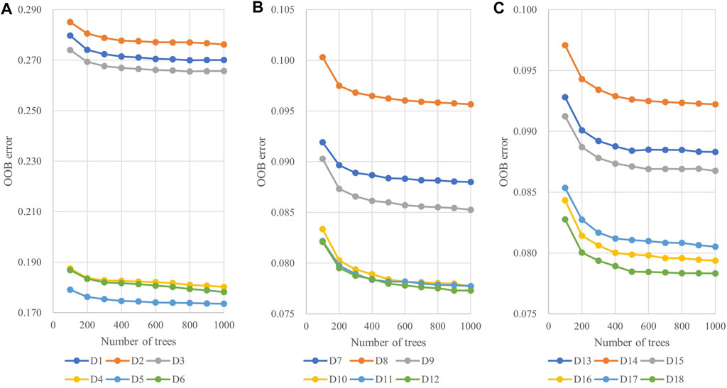
FIGURE 3. The average OOB error values for the number of trees (NT) of 18 datasets: (A) D1–D6; (B) D7–D12; and (C) D13–D18.

Figure 4 shows the average OOB error values of all 18 datasets at different BF when NT is 800. Regardless of the datasets used, OOB errors first decrease and then increase as the BF increases. For D1, D2, D3, and D5, the value of OOB reaches the minimum when the BF is around 0.6, while for other datasets, the value of OOB is the smallest when the BF is 0.9.

FIGURE 4

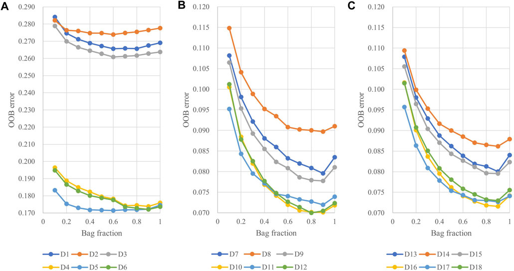
FIGURE 4. The average OOB error values for the bag fraction (BF) of 18 datasets: (A) D1–D6; (B) D7–D12; and (C) D13–D18.

Figure 5 shows the average OOB error values for all 18 datasets at different VPS when NT is 800. For D2, D5, D8, D11, D14, and D17, which only use season median or season median + auxiliary data, the OOB error showed a trend of decreasing at first and then increasing. For other data sets, OOB error shows a trend of decreasing and then tending to be stable with the increase of VPS value. The VPS value corresponding to the red solid circle in Figure 5 is the suggested value of GEE (square root of the number of variables). In Figure 5A, we found that when only the S1 data or S1+auxiliary data are used, the VPS value suggested by GEE is appropriate, and the OOB value obtained at this time is smaller. In Figures 5B, C, it is beneficial to use a VPS value larger than the GEE recommendation to reduce the value of OOB, especially for the four data sets D10, D12, D16 and D18. So, without loss of generality, we recommend using 1.5 times the square root of the number of variables as the value of VPS, as marked by the blue solid circle in the figure. At this time, the OBB errors of the 12 data sets D7-D18 are all small.

FIGURE 5

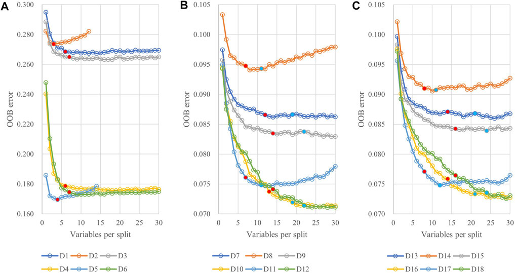
FIGURE 5. The average OOB error values for the variables per split (VPS) of 18 datasets: (A) D1–D6; (B) D7–D12; and (C) D13–D18.

Table 2 summarizes the optimal combination values for the parameter pair of VPS and BF with the smallest OOB error value when the NT value is set to 800. It was found that the optimal BF value was 0.9 for D7 to D18, see Table 2, which differs from the default value of BF (0.5) suggested by the GEE.

TABLE 2

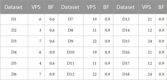
TABLE 2. Optimal combination values of VPS and BF.

3.2 LC classification in model area

The results of a LC classification in model area (Hefei City) in 2020 of 18 datasets (D1-D18) using the identified optimum parameters of the RF on the GEE are presented in Figure 6 and Table 3.

FIGURE 6

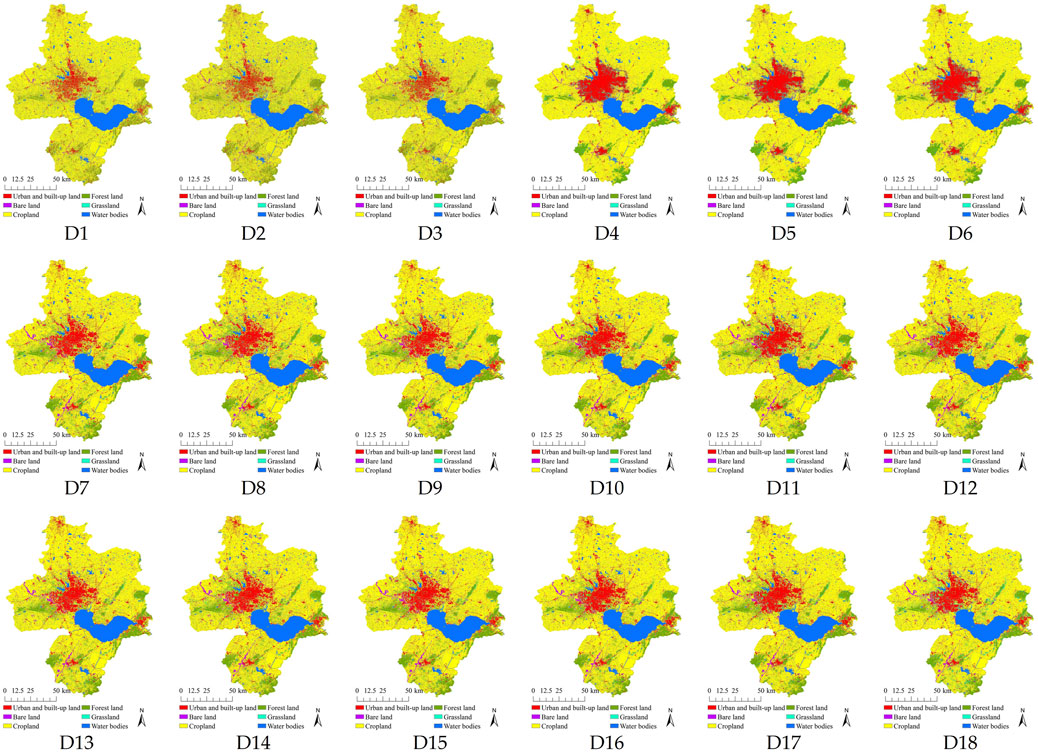
FIGURE 6. LC maps of Hefei City in 2020 of 18 datasets: D1–D18.

TABLE 3

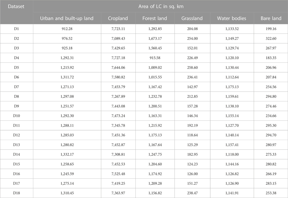
TABLE 3. Area of each LC type of 18 datasets: D1–D18.

As a result, in Figure 7, the patterns of LC distribution from 18 datasets are slightly different according to the number of features in the datasets. Likewise, the area of each LC type of 18 datasets in Table 3 is changed according to the number of features in the datasets. These phenomena can be clearly observed in each LC type change from 18 datasets (see Figure 7). Urban and built-up land areas are increased after adding auxiliary data to Sentinel-1 data (D1–D3), and they are relatively stable. Similarly, areas of forest land are stable using D7–D18 datasets. On the contrary, areas of cropland, grassland, water bodies, and bare land fluctuate for all 18 datasets.

FIGURE 7

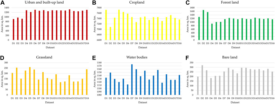
FIGURE 7. Change of each LC area from 18 datasets: (A) urban and built-up land, (B) cropland, (C) forest land, (D) grassland, (E) water bodies, and (F) bare land.

3.3 Thematic accuracy assessment of LC map in model area

The results of the OA and Kappa index for the thematic accuracy assessment of LC maps of 18 datasets (D1–D18) in model area (Hefei City) are presented in Figure 8. As a result, the OA values vary from 71.37% for D2 to 93.62% for D18, and the Kappa index values vary from 0.6017 for D2 to 0.9154 for D18.

FIGURE 8

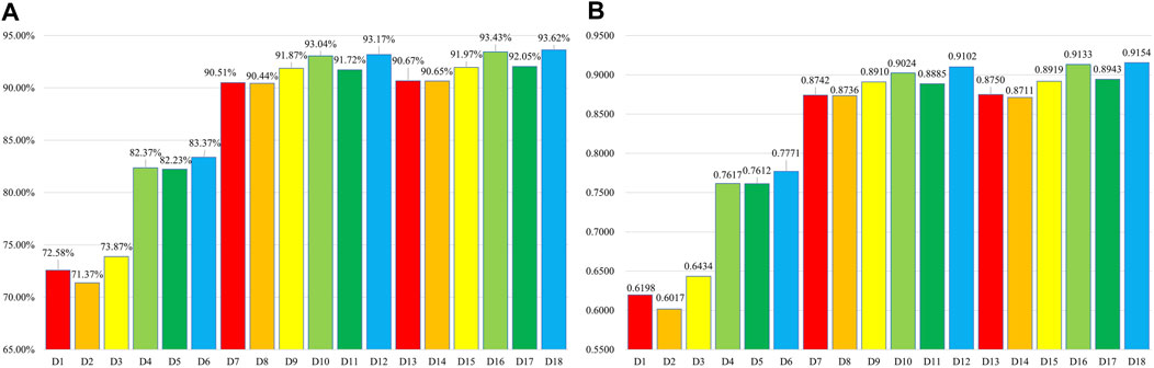
FIGURE 8. OA and Kappa index results for the 18 datasets: (A) OA and (B) Kappa index.

Meanwhile, the PA and UA values of each LC type are calculated on GEE. The PA values of urban and built-up land vary from about 51% for D2 to 95% for D18, the PA values of bare land vary from about 26% for D1 to 80% for D10, the PA values of cropland vary from about 89% for D2 to 98% for D10, the PA values of forest land vary from about 58% for D2 to 95% for D16, the PA values of grassland vary from about 12% for D1 to 82% for D12, and the PA values of water bodies vary from about 95% for D5 to 99% for D9. The UA values of urban and built-up land vary from about 67% for D3 to 93% for D12, the UA values of bare land vary from about 46% for D2 to 91% for D10, the UA values for cropland vary from about 69% for D2 to 93% for D18, the UA values of forest land vary from about 64% for D2 to 98% for D16, the UA values of grassland vary from about 45% for D2 to 95% for D18, and the UA values of water bodies vary from about 97% for D3 to 100% for D14 and D16.

In addition, the average PA and UA of three main data types of 18 datasets, S1 (D1–D6), S2 (D7–D12), and S1 and S2 (D13–D18), are summarized in Table 4.

TABLE 4

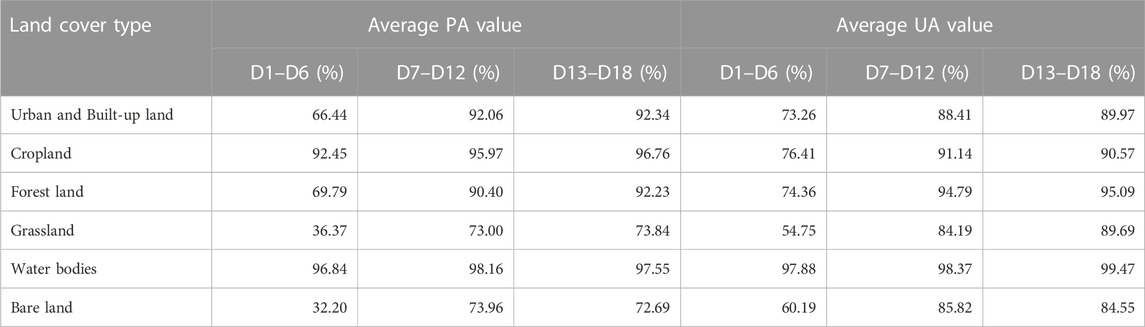
TABLE 4. Average PA and UA of three primary data types of 18 datasets (D1–D18).

For average PA in Table 4, the six datasets of S1 data (without and with auxiliary data), D1-D6, delivered average PA values from 32.20% for bare land to 96.84% for water bodies. On the contrary, the six datasets of S2 data (without and with auxiliary data), D7–D12, delivered average PA values from 73.00% for grassland to 98.16% for water bodies. Meanwhile, the six datasets of S1 and S2 data (without and with auxiliary data), D13–D18, delivered average PA values from 72.69% for bare land to 97.55% for water bodies.

Like PA, for average UA in Table 4, the six datasets of S1 data (without and with auxiliary data), D1-D6, delivered average UA values from 54.75% for grassland to 97.88% for water bodies. On the contrary, the six datasets of S2 data (without and with auxiliary data), D7-D12, delivered average UA values from 84.19% for grassland to 98.16% for water bodies. Meanwhile, the six datasets of S1 and S2 data (without and with auxiliary data), D13-D18, delivered average UA values from 84.55% for bare land to 99.47% for water bodies.

Furthermore, all six datasets of S1 data (without and with auxiliary data), (D1–D6), delivered a lower average PA and UA than the other two main data types.

3.4 Suitable data type for LC classification in model area

As summarized in Table 5, the OA, Kappa index, and the average value by data type for S2 data without auxiliary data (D7–D9) and with auxiliary data (D10–D12) were higher than that of S1 data without auxiliary data (D1–D3) and with auxiliary data (D4–D6). The average values of OA for the datasets of S2 data without and with auxiliary data were 90.94% and 92.64%, respectively, but the average values of OA for the datasets of S1 data without and with auxiliary data were only 72.61% and 82.66%, respectively. Likewise, the average values of the Kappa index for datasets of S2 data without and with auxiliary data were 0.8796 and 0.9004, respectively, but the average values of the Kappa index for datasets of S1 data without and with auxiliary data were only 0.6216 and 0.7667, respectively. Therefore, S2 data with and without auxiliary data were suitable for LC classification in terms of data type.

TABLE 5

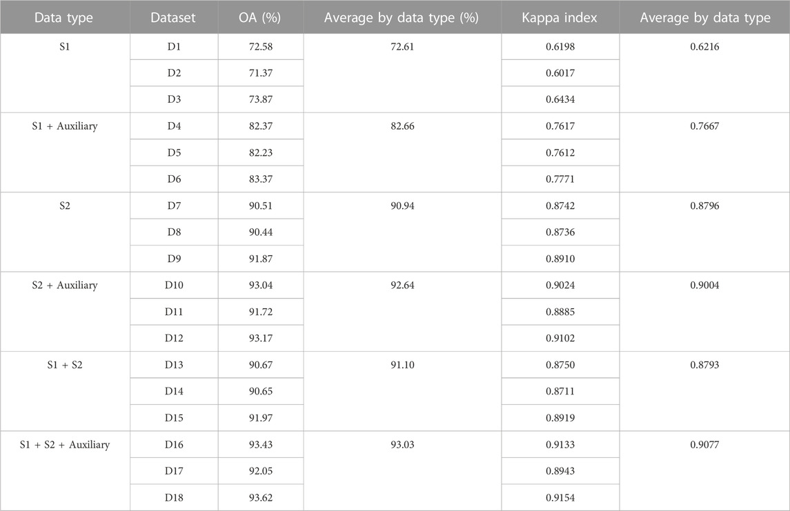
TABLE 5. OA, Kappa index, and average value by data type.

3.5 Suitable dataset for LC classification in model area

To identify a suitable dataset for LC classification, Kappa index values were compared among 18 datasets (see Table 5); the top three datasets, D18, D16, and D12, provided the highest Kappa index, with values of 0.9154, 0.9133, and 0.9102, respectively. On the contrary, three datasets, D3, D1, and D2, displayed the lowest Kappa index, with values of 0.6434, 0.6198, and 0.6017, respectively.

The z-statistic value for D12 and D16, D12 and D18, and D16 and D18 are 0.130737, 0.341274, and 0.208664, respectively, which are less than 1.28 (80% confidential level), 1.65 (90% confidential level), and 2.58 (100% confidential level). It means that when we consider the change of Kappa index value of top three datasets (D12, D16, and D18), the increasing of Kappa index of D16 and D18 is insignificant. So, D12 was selected as the suitable dataset for LC classification since we can reduce the time for preparing S1 data.

3.6 LC classification in test area

The results of LC classification in test area (Nanjing City) in 2020 from suitable data type (D7–D12) using RF on the GEE platform are presented in Figure 9 and Table 6.

FIGURE 9

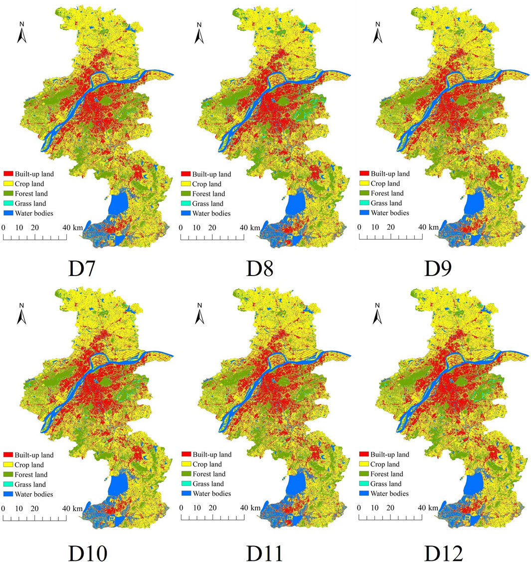
FIGURE 9. LC maps of Nanjing City in 2020 from datasets: D7–D12.

TABLE 6

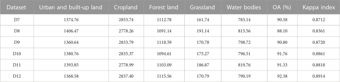
TABLE 6. Area of each LC type and OA and Kappa index results in Nanjing City in 2020.

As a result, in Figure 9, the patterns of LC distribution from 6 datasets are different according to the number of features in the datasets. Meanwhile, using the D7-D12 datasets, the areas of forest land are stable, while the areas of urban and built-up land, cropland, grassland, and water bodies fluctuate slightly (see Table 6).

Furthermore, thematic accuracy assessment of LC maps of 6 datasets (D7-D12) are presented in Table 6. The OA values vary from 88.10% for D8 to 92.38% for D12, and the Kappa index values vary from 0.8361 for D8 to 0.8914 for D12. As a result, the classified LC map in test area (Nanjing City) using the identified optimal parameters of RF from model area (Hefei city) with the suitable dataset can be accepted.

4 Discussion

4.1 Optimal parameters for RFs

Based on OOB error measurement, an optimal number of trees (NT) was 800 for balancing the efficiency and accuracy of the RF (see Figure 3). Meanwhile, the optimal combination values of VPS and BF of the RF algorithm for each dataset (D1–D18) were identified by trial and error with the smaller OOB error value, summarized in Table 2. The selection of a suitable NT and appropriate VPS and BF values can increase the classification accuracy of the RF classifier. This finding was consistent with the Svoboda’s (Svoboda et al., 2022) study that used the appropriate values of NT, VPS and BF of the RF for land use change and forestry in the Czech Republic.

4.2 Suitable data type and dataset for LC classification in model area

According to OA, the Kappa index, and the average value by data type in Table 5, S2 data without and with auxiliary data, D7–D9 and D10–D12, respectively, were suitable data types compared with S1 data without and with auxiliary data, D1–D3 and D4–D6, respectively. In this study, S2 data could distinguish between forest land and grassland better than S1 data since broad vegetation classes are discriminated more easily by their physiology using the optical sensor than their physical structure from the radar sensor. This finding is consistent with LC studies combining optical and radar data in other geographic regions (Vaglio Laurin et al., 2013; Stefanski et al., 2014).

For suitable dataset identification, when comparing the OA and Kappa index of 18 datasets, the top three datasets, D18, D16, and D12, provided the highest OA and Kappa index, as reported in Table 5. However, the derived Kappa index of three datasets were not significantly different according to pairwise Z test. This study selected D12 (S2 Monthly median + S2 Season median + DNB + Elevation), as the suitable dataset for LC classification. The combining S2 and auxiliary data could provide an OA and a Kappa index of 93.17% and 0.9102, respectively. This dataset was sufficient and acceptable to classify LC with high accuracy, as suggested by Anderson et al. (1976). and Rosenfield and Fitzpatrick-Lins, (1986).

4.3 LC classification and its accuracy in model area

As a result of LC classification in model area (Hefei City) shown in Figure 6 and Table 3, patterns of LC distribution and the area of each LC type were dependent on the selected features of each dataset (D1–D18). Meanwhile, the OA values of the 18 datasets varied from 71.37% to about 94%, and their Kappa index values varied from 0.6017 (or about 60%) to 0.9154 (or about 92%) (see Figure 8). The OA and Kappa index of LC maps from the D7–D18 dataset was higher than 85% and 0.8, respectively, indicating that the classification results are acceptable (Anderson et al., 1976; Rosenfield and Fitzpatrick-Lins, 1986). The results suggested that a dataset of S2 data without and with auxiliary data, D7–D12, could classify LC better than a dataset of S1 data without and with auxiliary data, D1–D6. The results are consistent with other studies (Gislason et al., 2006; Rodriguez-Galiano et al., 2012; Pelletier et al., 2016; Ghorbanian et al., 2020; Phan et al., 2020; Ghorbanian et al., 2021), that is, when classifying LC, the classification accuracy of S2 data is better than that of S1 data.

According to the results of PA and UA of each LC type (Supplementary Appendix S1, S2) and the average PA and UA of three primary data types of 18 datasets (Table 4), the derived values of PA and UA of each LC depend on the data type and its feature for LC classification using RF. In this study, water bodies can be classified with a highly accurate value of PA and UA in 18 datasets. Similarly, cropland can be classified with a highly accurate PA value in 18 datasets, while cropland can be classified with high accurate UA value in 15 datasets, but not in D1–D3. On the contrary, urban and built-up land, bare land, forest land, and grassland can be classified with highly accurate PA and UA values in 12 datasets, but not in D1–D6.

4.4 LC classification and its accuracy in test area

For the result of LC classification in the model area (Nanjing City) displayed in Figure 9 and Table 6, patterns of LC distribution and the area of each LC type also rely on the selected features of each dataset (D7-D12). In the meantime, the overall accuracy values of the six datasets fluctuated between 88.10% and 92.38%, and their Kappa index values varied from 0.8361 (or about 84%) to 0.8914 (or about 89%) (see Table 6). The OA and Kappa indexes of each LC maps from D7–D12 datasets were higher than 85% and 80% respectively, indicating that they can provide acceptable results (Anderson et al., 1976).

As a result, whether it is OA or Kappa index, the dataset of S2 data with auxiliary data (D10–D12) is higher than the dataset of S2 data without auxiliary data (D7–D9). In addition, datasets that adopt a combination of monthly median and season median (D9 and D12) have the highest OA and Kappa index, followed by the datasets using the monthly median (D7 and D10). Although datasets utilizing season median (D8 and D11) yield the lowest OA and Kappa, their values are still higher than 85% and 0.8, respectively, which are still acceptable results (Anderson et al., 1976).

4.5 Validation of optimal parameter of RF for LC classification

As far as the NT is concerned, there is a decreasing relationship between the value of OOB and the NT, which means that the more the NT, the more conducive to improving the classification accuracy, but the larger the value, the more memory and calculation time required, which affects the classification efficiency. In addition, the classification benefit brought by the increase in the NT also decreases as the NT increases. Therefore, it is vital to choose an appropriate NT. In this study, we choose 800 as a suitable value of NT, which is similar to the previous studies that set 300 or 500 (Nguyen et al., 2020; Fekri et al., 2021; Piao et al., 2021; Xiao et al., 2021; Yang et al., 2021).

As far as BF is concerned, the value of OOB and the value of BF show a relationship of decreasing at first and then increasing. For the D1, D2, D3, and D5 datasets, the most suitable BF value is about 0.6, while for other datasets (D6, D6, and D7–D18), the most suitable BF value is about 0.9, both of which are higher than the value suggested by GEE (0.5). This finding is consistent with Patrick’s (Kacic et al., 2021) work concluding that the classification accuracy is higher when the BF is equal to 0.9. But the finding is more different from the research (Svoboda et al., 2022), who set the value of bag fraction to 0.1 when using S2 for land use change and forestry.

For the value of VPS, the datasets using season median data or using season median data with auxiliary data (D2, D5, D8, D11, D14, and D17), there is a relationship of decrease at beginning and then increase between the value of VPS and the value of OOB. And the other 12 datasets show a decreasing relationship between the value of VPS and the value of OOB. In addition, the suitable values of VPS for these 18 different datasets are related to the number of features in the dataset. In this study, we choose 1.5 times square root of the number of features as the appropriate value, which is higher than GEE suggests 1 times square root of the number of features. This choice is consistent with the result of Patrick’s (Kacic et al., 2021) research proposing that the number of VPS holds positive correlations with classification accuracy. But the finding is slightly different from the research (Ghorbanian et al., 2021; Venter and Sydenham, 2021) using the value of VPS suggested by GEE.

As shown in Figure 8, the OA and Kappa index of the LC map in Hefei City using D12 as the dataset through RF under GEE are 93.17% and 0.9102, respectively. Meanwhile, in Table 6, the OA and Kappa index of the LC map in Nanjing City of D12 are 92.83% and 0.8914, respectively. The OA and Kappa index of the LC of the two cities are higher than 90% and 0.8, respectively, indicating that the appropriate data types, datasets and RF parameters obtained in this study have certain generalizability and can be applied to other cities.

4.6 Impact of Sentinel-2 data missing on LC classification

Since S2 data is susceptible to atmospheric influences, it is likely that some regions or some years do not have S2 median data during the rainy season. To study the effect of S2 median data missing on LC classification, taking the D7 dataset (OA = 90.51%) as a reference, the S2 median data of a certain month were artificially removed. We found that when the median data of S2 in any month are missing, the OA does not change much, and the change of OA is within ±1%. OA decreased the most (−0.83%) when the median data for June were missing, and OA improved the most (+0.94%) when the median data for July were missing. The possible reason is that there were more cloudy and rainy days in July, and some cloud coverage pixels were not identified by the QA band, which cause the data in July to play a negative role in the LU classification. Taking the D8 dataset (OA = 90.44%) as a reference, the S2 median data of a certain season were artificially removed. We found that when the median data of Spring, Summer, Autumn, and Winter were missing, the OA changed to 90.62%, 88.71%, 89.98%, and 90.22%. It shows that the median data of Spring have a slight negative impact on the classification of LC. The median data of Summer are more important than other seasons, and when the data are missing, the classification accuracy of LC is reduced by about 1.7%. This shows that median data of Summer are more important for LC classification, but at the same time, it should be noted that the quality of data in some months of Summer may be low. So, accurate identification of cloud contamination pixels is conducive to improving the OA of LC classification.

4.7 Strength and limitation of google earth engine

GEE’s data archive contains more than 40 years of historical datasets that are updated and expanded daily, including the Landsat, Sentinel, MODIS, land cover data, and so on. GEE also provides a variety of ML classification algorithms, such as CART, RF, SVM, naive Bayes, and decision tree. Since it is cloud-based, there is no need to download a large number of image files, and when the relevant parameters are set, the classification results of city-scale LC can be obtained within a few minutes. When running analytics on platforms like ERDAS and ENVI, it can take hours or even days to download the data and process the analytics. Therefore, the research method developed based on GEE can be applied to the update of LC maps where LC changes quickly occur. However, GEE is also limited in some cases, such as memory overflow, and other cloud platforms such as Amazon Web Services and Pixel Information Expert (PIE) Engine can be tried in the future.

5 Conclusion

In recent years, the advantages of GEE’s abundance of available data and fast processing of remote sensing data have facilitated the remarkable development of RF algorithm for LC classification. To this end, it is crucial to investigate suitable data types, datasets, and input parameters of RF for LC classification.

This study classifies the LC of the model area (Hefei City) and evaluates the accuracy to determine the suitable data types, datasets and RF input parameters. The results show that the OA, Kappa index, PA and UA of all six datasets of S2 data (D7–D12) are higher than that of S1 data (D1–D6).

Meanwhile, the most suitable dataset for LC classification is D12, which combines S2 and auxiliary data. The OA and Kappa index of Hefei City reach 93.17% and 0.9102, respectively, when the values of the three primary parameters NT, VPS and BF of RF are 800, 22 and 0.9, respectively. Then, the suitable dataset and parameters of the RF obtained in the model area (Hefei City) were verified in a test area (Nanjing City). The results show that the OA and Kappa index of Nanjing City are 92.38% and 0.8914 respectively. The OA and Kappa index of LC in Nanjing City and Hefei City are higher than 90% and 0.85 respectively, and the OAs are also higher than the accuracies reported by the LC products data providers themselves: ESA WorldCover reported 74%; ESRI Land Cover reported 85% (Venter et al., 2022). It turns out that based on the suitable data type obtained from the model area (Hefei City), the dataset and the input parameters of the RF can be generalized to test area (Nanjing City). In conclusion, the proposed method and the appropriate data types, datasets and RF parameters obtained in this study have certain universality and reference, and can be used to update the local LC information in other cities at low cost and high speed in the future. However, LC classification usually depends heavily on samples, data and algorithms. In future work, we will study sample generation strategies based on data distribution characteristics, open source databases, and existing land cover products; data integration techniques on the basis of multi-scale, multi-platform, and multi-modal; and algorithm integration of various ML and DL algorithms.

Data availability statement

Publicly available datasets were analyzed in this study. This data can be found here: https://developers.google.com/earth-engine/datasets/catalog/NOAA_VIIRS_DNB_MONTHLY_V1_VCMCFG?hl=en, https://developers.google.com/earth-engine/datasets/catalog/ESA_WorldCover_v100, https://developers.google.com/earth-engine/datasets/catalog/COPERNICUS_S1_GRD, https://developers.google.com/earth-engine/datasets/catalog/COPERNICUS_S2_SR, https://livingatlas.arcgis.com/landcover/, https://developers.google.com/earth-engine/datasets/catalog/USGS_SRTMGL1_003?hl=en.

Author contributions

JS: Conceptualization, methodology, software, validation, formal analysis, investigation, resources, data curation, original draft preparation, visualization, project administration, funding acquisition. SO: Conceptualization, methodology, validation, review and editing, supervision. All authors contributed to the article and approved the submitted version.

Funding

This research was funded by the Natural Science Research Project of the Anhui Education Department, grant number KJ2019A0707.

Acknowledgments

The facility support from Tongling University is gratefully acknowledged by the authors. Special thanks from the authors go to the reviewers for their valuable comments and suggestions that improved our manuscript from various perspectives.

Conflict of interest

The authors declare that the research was conducted in the absence of any commercial or financial relationships that could be construed as a potential conflict of interest.

Publisher’s note

All claims expressed in this article are solely those of the authors and do not necessarily represent those of their affiliated organizations, or those of the publisher, the editors and the reviewers. Any product that may be evaluated in this article, or claim that may be made by its manufacturer, is not guaranteed or endorsed by the publisher.

Supplementary material

The Supplementary Material for this article can be found online at: https://www.frontiersin.org/articles/10.3389/feart.2023.1188093/full#supplementary-material

References

Amani, M., Ghorbanian, A., Ahmadi, S. A., Kakooei, M., Moghimi, A., Mirmazloumi, S. M., et al. (2020). Google Earth engine cloud computing platform for remote sensing big data applications: a comprehensive review. IEEE J. Sel. Top. Appl. Earth Observations Remote Sens. 13, 5326–5350. doi:10.1109/jstars.2020.3021052

CrossRef Full Text | Google Scholar

Anderson, J. R., Hardy, E. E., Roach, J. T., and Witmer, R. E. (1976). A land use and land cover classification system for use with remote sensor data. Professional Paper. -.

CrossRef Full Text | Google Scholar

Azzari, G., and Lobell, D. B. (2017). Landsat-based classification in the cloud: an opportunity for a paradigm shift in land cover monitoring. Remote Sens. Environ. 202, 64–74. doi:10.1016/j.rse.2017.05.025

CrossRef Full Text | Google Scholar

Ban, Y., Webber, L., Gamba, P., and Paganini, M. (2017). Joint urban remote sensing event (JURSE), 6-8 march 2017 2017, 1–4.EO4Urban: sentinel-1A SAR and Sentinel-2A MSI data for global urban services

CrossRef Full Text | Google Scholar

Bourgoin, C., Oszwald, J., Bourgoin, J., Gond, V., Blanc, L., Dessard, H., et al. (2020). Assessing the ecological vulnerability of forest landscape to agricultural frontier expansion in the Central Highlands of Vietnam. Int. J. Appl. Earth Observation Geoinformation 84, 101958. doi:10.1016/j.jag.2019.101958

CrossRef Full Text | Google Scholar

Breiman, L. (2001). Random forests. Mach. Learn. 45, 5–32. doi:10.1023/a:1010933404324

CrossRef Full Text | Google Scholar

Chatziantoniou, A., Psomiadis, E., and Petropoulos, G. P. (2017). Co-orbital sentinel 1 and 2 for LULC mapping with emphasis on wetlands in a mediterranean setting based on machine learning. Remote Sens. 9, 1259. doi:10.3390/rs9121259

CrossRef Full Text | Google Scholar

Chen, J., Chen, J., Liao, A., Cao, X., Chen, L., Chen, X., et al. (2015). Global land cover mapping at 30m resolution: a POK-based operational approach. ISPRS J. Photogrammetry Remote Sens. 103, 7–27. doi:10.1016/j.isprsjprs.2014.09.002

CrossRef Full Text | Google Scholar

Chen, Y., Wang, Y., Gu, Y., He, X., Ghamisi, P., and Jia, X. (2019). Deep learning ensemble for hyperspectral image classification. IEEE J. Sel. Top. Appl. Earth Observations Remote Sens. 12, 1882–1897. doi:10.1109/jstars.2019.2915259

CrossRef Full Text | Google Scholar

Clark, M. L. (2017). Comparison of simulated hyperspectral HyspIRI and multispectral Landsat 8 and Sentinel-2 imagery for multi-seasonal, regional land-cover mapping. Remote Sens. Environ. 200, 311–325. doi:10.1016/j.rse.2017.08.028

CrossRef Full Text | Google Scholar

Clerici, N., Valbuena CalderóN, C. A., and Posada, J. M. (2017). Fusion of Sentinel-1A and Sentinel-2A data for land cover mapping: a case study in the lower Magdalena region, Colombia. J. Maps 13, 718–726. doi:10.1080/17445647.2017.1372316

CrossRef Full Text | Google Scholar

Congalton, R. G., and Green, K. (2009). Assessing the accuracy of remotely sensed data - principles and practices. Second edition. Boca Raton, NW, USA: CRC Press, Taylor & Francis Group.

Google Scholar

Cremer, F., Urbazaev, M., CortéS, J., Truckenbrodt, J., Schmullius, C., and Thiel, C. (2020). “Potential of recurrence metrics from sentinel-1 time series for deforestation mapping,” in IEEE Journal of Selected Topics in Applied Earth Observations and Remote Sensing, 13, 5233–5240. doi:10.1109/jstars.2020.3019333

PubMed Abstract | CrossRef Full Text | Google Scholar

Defries, R. (2008). Terrestrial vegetation in the coupled human-earth system: contributions of remote sensing. Annu. Rev. Environ. Resour. 33, 369–390. doi:10.1146/annurev.environ.33.020107.113339

CrossRef Full Text | Google Scholar

Drusch, M., Del Bello, U., Carlier, S., Colin, O., Fernandez, V., Gascon, F., et al. (2012). Sentinel-2: ESA's optical high-resolution mission for GMES operational services. Remote Sens. Environ. 120, 25–36. doi:10.1016/j.rse.2011.11.026

CrossRef Full Text | Google Scholar

EOG (2023). Earth observation group. Payne Institute for Public Policy, Colorado School of Mines. Available: https://developers.google.com/earth-engine/datasets/catalog/NOAA_VIIRS_DNB_MONTHLY_V1_VCMCFG?hl=en (Accessed February 16, 2023).VIIRS nighttime day/night band composites version 1.

Google Scholar

Erasmi, S., and Twele, A. (2009). Regional land cover mapping in the humid tropics using combined optical and SAR satellite data—a case study from Central Sulawesi, Indonesia. Int. J. Remote Sens. 30, 2465–2478. doi:10.1080/01431160802552728

CrossRef Full Text | Google Scholar

ESA (2023a). ESA WorldCover 10m v100. Available: https://developers.google.com/earth-engine/datasets/catalog/ESA_WorldCover_v100 (Accessed February 16, 2023).

Google Scholar

ESA (2023b). Sentinel-1 SAR GRD. Available: https://developers.google.com/earth-engine/datasets/catalog/COPERNICUS_S1_GRD (Accessed February 16, 2023).

Google Scholar

ESA (2023c). Sentinel-2 MSI. Available: https://developers.google.com/earth-engine/datasets/catalog/COPERNICUS_S2_SR (Accessed February, 2023).

Google Scholar

ESRI (2023). Esri land cover. Available: https://livingatlas.arcgis.com/landcover/ (Accessed February 16, 2023).

Google Scholar

Feddema, J. J., Oleson, K. W., Bonan, G. B., Mearns, L. O., Buja, L. E., Meehl, G. A., et al. (2005). The importance of land-cover change in simulating future climates. Science 310, 1674–1678. doi:10.1126/science.1118160

PubMed Abstract | CrossRef Full Text | Google Scholar

Fekri, E., Latifi, H., Amani, M., and Zobeidinezhad, A. (2021). A training sample migration method for wetland mapping and monitoring using sentinel data in Google Earth engine. Remote Sens. 13, 4169. doi:10.3390/rs13204169

CrossRef Full Text | Google Scholar

Forkuor, G., Dimobe, K., Serme, I., and Tondoh, J. E. (2018). Landsat-8 vs. Sentinel-2: examining the added value of sentinel-2’s red-edge bands to land-use and land-cover mapping in Burkina Faso. GIScience Remote Sens. 55, 331–354. doi:10.1080/15481603.2017.1370169

CrossRef Full Text | Google Scholar

Freitas, C. D. C., Soler, L. D. S., San” Anna, S. J. S., Dutra, L. V., Santos, J. R. D., Mura, J. C., et al. (2008). Land use and land cover mapping in the Brazilian Amazon using polarimetric airborne P-band SAR data. IEEE Trans. Geoscience Remote Sens. 46, 2956–2970. doi:10.1109/tgrs.2008.2000630

CrossRef Full Text | Google Scholar

Gao, B.-C. (1996). NDWI—a normalized difference water index for remote sensing of vegetation liquid water from space. Remote Sens. Environ. 58, 257–266. doi:10.1016/s0034-4257(96)00067-3

CrossRef Full Text | Google Scholar

Ghorbanian, A., Kakooei, M., Amani, M., Mahdavi, S., Mohammadzadeh, A., and Hasanlou, M. (2020). Improved land cover map of Iran using Sentinel imagery within Google Earth Engine and a novel automatic workflow for land cover classification using migrated training samples. ISPRS J. Photogrammetry Remote Sens. 167, 276–288. doi:10.1016/j.isprsjprs.2020.07.013

CrossRef Full Text | Google Scholar

Ghorbanian, A., Zaghian, S., Asiyabi, R. M., Amani, M., Mohammadzadeh, A., and Jamali, S. (2021). Mangrove ecosystem mapping using sentinel-1 and sentinel-2 satellite images and random forest algorithm in Google Earth engine. Remote Sens. 13, 2565. doi:10.3390/rs13132565

CrossRef Full Text | Google Scholar

Gislason, P. O., Benediktsson, J. A., and Sveinsson, J. R. (2006). Random Forests for land cover classification. Pattern Recognit. Lett. 27, 294–300. doi:10.1016/j.patrec.2005.08.011

CrossRef Full Text | Google Scholar

Goldblatt, R., Stuhlmacher, M. F., Tellman, B., Clinton, N., Hanson, G., Georgescu, M., et al. (2018). Using Landsat and nighttime lights for supervised pixel-based image classification of urban land cover. Remote Sens. Environ. 205, 253–275. doi:10.1016/j.rse.2017.11.026

CrossRef Full Text | Google Scholar

GóMEZ, C., White, J. C., and Wulder, M. A. (2016). Optical remotely sensed time series data for land cover classification: a review. ISPRS J. Photogrammetry Remote Sens. 116, 55–72. doi:10.1016/j.isprsjprs.2016.03.008

CrossRef Full Text | Google Scholar

Gong, P., Liu, H., Zhang, M., Li, C., Wang, J., Huang, H., et al. (2019). Stable classification with limited sample: transferring a 30-m resolution sample set collected in 2015 to mapping 10-m resolution global land cover in 2017. Sci. Bull. 64, 370–373. doi:10.1016/j.scib.2019.03.002

PubMed Abstract | CrossRef Full Text | Google Scholar

Gong, P., Wang, J., Yu, L., Zhao, Y., Zhao, Y., Liang, L., et al. (2013). Finer resolution observation and monitoring of global land cover: first mapping results with Landsat TM and ETM+ data. Int. J. Remote Sens. 34, 2607–2654. doi:10.1080/01431161.2012.748992

CrossRef Full Text | Google Scholar

Gorelick, N., Hancher, M., Dixon, M., Ilyushchenko, S., Thau, D., and Moore, R. (2017). Google Earth Engine: planetary-scale geospatial analysis for everyone. Remote Sens. Environ. 202, 18–27. doi:10.1016/j.rse.2017.06.031

CrossRef Full Text | Google Scholar

Hansen, M. C., and Loveland, T. R. (2012). A review of large area monitoring of land cover change using Landsat data. Remote Sens. Environ. 122, 66–74. doi:10.1016/j.rse.2011.08.024

CrossRef Full Text | Google Scholar

Hong, D., Gao, L., Yao, J., Zhang, B., Plaza, A., and Chanussot, J. (2021a). Graph convolutional networks for hyperspectral image classification. IEEE Trans. Geoscience Remote Sens. 59, 5966–5978. doi:10.1109/tgrs.2020.3015157

CrossRef Full Text | Google Scholar

Hong, D., Gao, L., Yokoya, N., Yao, J., Chanussot, J., Du, Q., et al. (2021b). More diverse means better: multimodal deep learning meets remote-sensing imagery classification. IEEE Trans. Geoscience Remote Sens. 59, 4340–4354. doi:10.1109/tgrs.2020.3016820

CrossRef Full Text | Google Scholar

Huang, D., Xu, S., Sun, J., Liang, S., Song, W., and Wang, Z. (2017). Accuracy assessment model for classification result of remote sensing image based on spatial sampling. J. Appl. Remote Sens. 11, 1. doi:10.1117/1.jrs.11.046023

CrossRef Full Text | Google Scholar

Joshi, N., Baumann, M., Ehammer, A., Fensholt, R., Grogan, K., Hostert, P., et al. (2016). A review of the application of optical and radar remote sensing data fusion to land use mapping and monitoring. Remote Sens. 8, 70. doi:10.3390/rs8010070

CrossRef Full Text | Google Scholar

Ju, J., and Roy, D. P. (2008). The availability of cloud-free Landsat ETM+ data over the conterminous United States and globally. Remote Sens. Environ. 112, 1196–1211. doi:10.1016/j.rse.2007.08.011

CrossRef Full Text | Google Scholar

Kacic, P., Hirner, A., and Da Ponte, E. (2021). Fusing sentinel-1 and -2 to model GEDI-derived vegetation structure characteristics in GEE for the Paraguayan chaco. Remote Sens. 13, 5105. doi:10.3390/rs13245105

CrossRef Full Text | Google Scholar

Klaiber, M. (2021). A fundamental overview of SOTA-ensemble learning methods for deep learning. A Syst. Lit. Rev. 2, 14. doi:10.31763/sitech.v2i2.549

CrossRef Full Text | Google Scholar

Krishna, K., Caitlin, K., Zoe, S.-W., Joseph, M., Mark, M., and Steven, B.IMPACT OBSERVATORY, UNITED STATES (2021). “Global land use/land cover with Sentinel-2 and deep learning,” in IGARSS 2021-2021 IEEE International Geoscience and Remote Sensing Symposium.

Google Scholar

Kumar, L., and Mutanga, O. (2018). Google Earth engine applications since inception: usage, trends, and potential. Remote Sens. 10, 1509. doi:10.3390/rs10101509

CrossRef Full Text | Google Scholar

Lin, Q., Guo, J., Yan, J., and Heng, W. (2018). Land use and landscape pattern changes of Weihai, China based on object-oriented SVM classification from Landsat MSS/TM/OLI images. Eur. J. Remote Sens. 51, 1036–1048. doi:10.1080/22797254.2018.1534532

CrossRef Full Text | Google Scholar

Liu, C., Li, W., Zhu, G., Zhou, H., Yan, H., and Xue, P. (2020a). Land use/land cover changes and their driving factors in the northeastern Tibetan plateau based on geographical detectors and Google Earth engine: a case study in gannan prefecture. Remote Sens. 12, 3139. doi:10.3390/rs12193139

CrossRef Full Text | Google Scholar

Liu, H., Gong, P., Wang, J., Clinton, N., Bai, Y., and Liang, S. (2020b). Annual dynamics of global land cover and its long-term changes from 1982 to 2015. Earth Syst. Sci. Data 12, 1217–1243. doi:10.5194/essd-12-1217-2020

CrossRef Full Text | Google Scholar

Luo, J., Ma, X., Chu, Q., Xie, M., and Cao, Y. (2021). Characterizing the up-to-date land-use and land-cover change in xiong’an new area from 2017 to 2020 using the multi-temporal sentinel-2 images on Google Earth engine. ISPRS Int. J. Geo-Information 10, 464. doi:10.3390/ijgi10070464

CrossRef Full Text | Google Scholar

Lyons, M. B., Keith, D. A., Phinn, S. R., Mason, T. J., and Elith, J. (2018). A comparison of resampling methods for remote sensing classification and accuracy assessment. Remote Sens. Environ. 208, 145–153. doi:10.1016/j.rse.2018.02.026

CrossRef Full Text | Google Scholar

Masroor, M., Avtar, R., Sajjad, H., Choudhari, P., Kulimushi, L. C., Khedher, K. M., et al. (2022). Assessing the influence of land use/land cover alteration on climate variability: an analysis in the aurangabad district of Maharashtra state, India. Sustainability 14, 642. doi:10.3390/su14020642

CrossRef Full Text | Google Scholar

Miller, S. D., Straka, W., Mills, S. P., Elvidge, C. D., Lee, T. F., Solbrig, J., et al. (2013). Illuminating the capabilities of the suomi national polar-orbiting partnership (NPP) visible infrared imaging radiometer suite (VIIRS) day/night band. Remote Sens. 5, 6717–6766. doi:10.3390/rs5126717

CrossRef Full Text | Google Scholar

Mongus, D., and Žalik, B. (2018). Segmentation schema for enhancing land cover identification: a case study using Sentinel 2 data. Int. J. Appl. Earth Observation Geoinformation 66, 56–68. doi:10.1016/j.jag.2017.11.004

CrossRef Full Text | Google Scholar

Mutanga, O., and Kumar, L. (2019). Google Earth engine applications. Remote Sens. 11, 591. doi:10.3390/rs11050591

CrossRef Full Text | Google Scholar

NASA (2023). NASA SRTM Digital Elevation 30m. Available: https://developers.google.com/earth-engine/datasets/catalog/USGS_SRTMGL1_003?hl=en (Accessed February 16, 2023).

Google Scholar

Nguyen, H. T. T., Doan, T. M., Tomppo, E., and Mcroberts, R. E. (2020). Land use/land cover mapping using multitemporal sentinel-2 imagery and four classification methods—a case study from dak nong, vietnam. Remote Sens. 12, 1367. doi:10.3390/rs12091367

CrossRef Full Text | Google Scholar

Pelletier, C., Valero, S., Inglada, J., Champion, N., and Dedieu, G. (2016). Assessing the robustness of Random Forests to map land cover with high resolution satellite image time series over large areas. Remote Sens. Environ. 187, 156–168. doi:10.1016/j.rse.2016.10.010

CrossRef Full Text | Google Scholar

Pesaresi, M., Corbane, C., Julea, A., Florczyk, A. J., Syrris, V., and Soille, P. (2016). Assessment of the added-value of sentinel-2 for detecting built-up areas. Remote Sens. 8, 299. doi:10.3390/rs8040299

CrossRef Full Text | Google Scholar

Phan, T. N., Kuch, V., and Lehnert, L. W. (2020). Land cover classification using Google Earth engine and random forest classifier—the role of image composition. Remote Sens. 12, 2411. doi:10.3390/rs12152411

CrossRef Full Text | Google Scholar

Piao, Y., Jeong, S., Park, S., and Lee, D. (2021). Analysis of land use and land cover change using time-series data and random forest in North Korea. Remote Sens. 13, 3501. doi:10.3390/rs13173501

CrossRef Full Text | Google Scholar

Pirotti, F., Sunar, F., and Piragnolo, M. (2016). Benchmark of machine learning methods for classification of a Sentinel-2 image. Int. Arch. Photogramm. Remote Sens. Spat. Inf. Sci., 335–340. doi:10.5194/isprsarchives-xli-b7-335-2016

CrossRef Full Text | Google Scholar

Ray, S. (2019). “A quick review of machine learning algorithms,” in International Conference on Machine Learning, Big Data, Cloud and Parallel Computing (COMITCon), 14-16 Feb. 2019, 35–39.

CrossRef Full Text | Google Scholar

Rodriguez-Galiano, V. F., Ghimire, B., Rogan, J., Chica-Olmo, M., and Rigol-Sanchez, J. P. (2012). An assessment of the effectiveness of a random forest classifier for land-cover classification. ISPRS J. Photogrammetry Remote Sens. 67, 93–104. doi:10.1016/j.isprsjprs.2011.11.002

CrossRef Full Text | Google Scholar

Rosenfield, G. H., and Fitzpatrick-Lins, K. (1986). A coefficient of agreement as a measure of thematic classification accuracy. Photogramm. Eng. remote Sens. 52, 223–227.

Google Scholar

Shelestov, A., Lavreniuk, M., Kussul, N., Novikov, A., and Skakun, S. (2017). Exploring Google Earth engine platform for big data processing: classification of multi-temporal satellite imagery for crop mapping. Front. Earth Sci. 5. doi:10.3389/feart.2017.00017

CrossRef Full Text | Google Scholar

Shetty, S., Gupta, P. K., Belgiu, M., and Srivastav, S. K. (2021). Assessing the effect of training sampling design on the performance of machine learning classifiers for land cover mapping using multi-temporal remote sensing data and Google Earth engine. Remote Sens. 13, 1433. doi:10.3390/rs13081433

CrossRef Full Text | Google Scholar

Shrestha, A., and Mahmood, A. (2019). Review of deep learning algorithms and architectures. IEEE Access 7, 53040–53065. doi:10.1109/access.2019.2912200

CrossRef Full Text | Google Scholar

Soenen, S. A., Peddle, D. R., and Coburn, C. A. (2005). SCS+C: a modified Sun-canopy-sensor topographic correction in forested terrain. IEEE Trans. Geoscience Remote Sens. 43, 2148–2159. doi:10.1109/tgrs.2005.852480

CrossRef Full Text | Google Scholar

Song, X.-P., Hansen, M. C., Stehman, S. V., Potapov, P. V., Tyukavina, A., Vermote, E. F., et al. (2018). Global land change from 1982 to 2016. Nature 560, 639–643. doi:10.1038/s41586-018-0411-9

PubMed Abstract | CrossRef Full Text | Google Scholar

Sothe, C., Almeida, C. M. D., Liesenberg, V., and Schimalski, M. B. (2017). Evaluating sentinel-2 and landsat-8 data to map sucessional forest stages in a subtropical forest in southern Brazil. Remote Sens. 9, 838. doi:10.3390/rs9080838

CrossRef Full Text | Google Scholar

Spoto, F., Sy, O., Laberinti, P., Martimort, P., Fernandez, V., Colin, O., et al. (2012). “Overview of sentinel-2,” in 2012 IEEE International Geoscience and Remote Sensing Symposium, 22-27 July 2012, 1707–1710.

Google Scholar

Stefanski, J., Kuemmerle, T., Chaskovskyy, O., Griffiths, P., Havryluk, V., Knorn, J., et al. (2014). Mapping land management regimes in western Ukraine using optical and SAR data. Remote Sens. 6, 5279–5305. doi:10.3390/rs6065279

CrossRef Full Text | Google Scholar

Su, Y., Li, X., Feng, M., Nian, Y., Huang, L., Xie, T., et al. (2021). High agricultural water consumption led to the continued shrinkage of the Aral Sea during 1992–2015. Sci. Total Environ. 777, 145993. doi:10.1016/j.scitotenv.2021.145993

PubMed Abstract | CrossRef Full Text | Google Scholar

Sun, Z., Di, L., and Fang, H. (2019). Using long short-term memory recurrent neural network in land cover classification on Landsat and Cropland data layer time series. Int. J. Remote Sens. 40, 593–614. doi:10.1080/01431161.2018.1516313

CrossRef Full Text | Google Scholar

Svoboda, J., Štych, P., Laštovička, J., Paluba, D., and Kobliuk, N. (2022). Random forest classification of land use, land-use change and forestry (LULUCF) using sentinel-2 data—a case study of Czechia. Remote Sens. 14, 1189. doi:10.3390/rs14051189

CrossRef Full Text | Google Scholar

Tamiminia, H., Salehi, B., Mahdianpari, M., Quackenbush, L., Adeli, S., and Brisco, B. (2020). Google Earth Engine for geo-big data applications: a meta-analysis and systematic review. ISPRS J. Photogrammetry Remote Sens. 164, 152–170. doi:10.1016/j.isprsjprs.2020.04.001

CrossRef Full Text | Google Scholar

Tang, P., Du, P., Lin, C., Guo, S., and Qie, L. (2020). A novel sample selection method for impervious surface area mapping using JL1-3B nighttime light and sentinel-2 imagery. IEEE J. Sel. Top. Appl. Earth Observations Remote Sens. 13, 3931–3941. doi:10.1109/jstars.2020.3004654

CrossRef Full Text | Google Scholar

Thanh Noi, P., and Kappas, M. (2018). Comparison of random forest, k-nearest neighbor, and support vector machine classifiers for land cover classification using sentinel-2 imagery. Sensors 18, 18. doi:10.3390/s18010018

CrossRef Full Text | Google Scholar

Torres, R., Snoeij, P., Geudtner, D., Bibby, D., Davidson, M., Attema, E., et al. (2012). GMES Sentinel-1 mission. Remote Sens. Environ. 120, 9–24. doi:10.1016/j.rse.2011.05.028

CrossRef Full Text | Google Scholar

Tucker, C. J. (1979). Red and photographic infrared linear combinations for monitoring vegetation. Remote Sens. Environ. 8, 127–150. doi:10.1016/0034-4257(79)90013-0

CrossRef Full Text | Google Scholar

Turner, B. L., Lambin, E. F., and Reenberg, A. (2007). The emergence of land change science for global environmental change and sustainability. Proc. Natl. Acad. Sci. 104, 20666–20671. doi:10.1073/pnas.0704119104

PubMed Abstract | CrossRef Full Text | Google Scholar

Vaglio Laurin, G., Liesenberg, V., Chen, Q., Guerriero, L., Del Frate, F., Bartolini, A., et al. (2013). Optical and SAR sensor synergies for forest and land cover mapping in a tropical site in West Africa. Int. J. Appl. Earth Observation Geoinformation 21, 7–16. doi:10.1016/j.jag.2012.08.002

CrossRef Full Text | Google Scholar

Venter, Z. S., Barton, D. N., Chakraborty, T., Simensen, T., and Singh, G. (2022). Global 10 m land use land cover datasets: a comparison of dynamic World, World cover and esri land cover. Remote Sens. 14, 4101. doi:10.3390/rs14164101

CrossRef Full Text | Google Scholar

Venter, Z. S., and Sydenham, M. A. K. (2021). Continental-scale land cover mapping at 10 m resolution over europe (ELC10). Remote Sens. 13, 2301. doi:10.3390/rs13122301

CrossRef Full Text | Google Scholar

Wu, X., Hong, D., and Chanussot, J. (2022). Convolutional neural networks for multimodal remote sensing data classification. IEEE Trans. Geoscience Remote Sens. 60, 1–10. doi:10.1109/tgrs.2021.3124913

CrossRef Full Text | Google Scholar

Xiao, W., Xu, S., and He, T. (2021). Mapping paddy rice with sentinel-1/2 and phenology-object-based algorithm—a implementation in hangjiahu plain in China using GEE platform. Remote Sens. 13, 990. doi:10.3390/rs13050990

CrossRef Full Text | Google Scholar

Yang, Y., Yang, D., Wang, X., Zhang, Z., and Nawaz, Z. (2021). Testing accuracy of land cover classification algorithms in the qilian mountains based on GEE cloud platform. Remote Sens. 13, 5064. doi:10.3390/rs13245064

CrossRef Full Text | Google Scholar

Zanaga, D., Van De Kerchove, R., De Keersmaecker, W., Souverijns, N., Brockmann, C., Quast, R., et al. (2021). ESA WorldCover 10 m 2020 v100.

Google Scholar

Zeng, H., Wu, B., Wang, S., Musakwa, W., Tian, F., Mashimbye, Z. E., et al. (2020). A synthesizing land-cover classification method based on Google Earth engine: a case study in nzhelele and levhuvu catchments, South Africa. Chin. Geogr. Sci. 30, 397–409. doi:10.1007/s11769-020-1119-y

CrossRef Full Text | Google Scholar

Zha, Y., Gao, J., and Ni, S. (2003). Use of normalized difference built-up index in automatically mapping urban areas from TM imagery. Int. J. Remote Sens. 24, 583–594. doi:10.1080/01431160304987

CrossRef Full Text | Google Scholar

Zhang, M., Huang, H., Li, Z., Hackman, K. O., Liu, C., Andriamiarisoa, R. L., et al. (2020). Automatic high-resolution land cover production in Madagascar using sentinel-2 time series, tile-based image classification and Google Earth engine. Remote Sens. 12, 3663. doi:10.3390/rs12213663

CrossRef Full Text | Google Scholar

Zhang, X., Liu, L., Chen, X., Gao, Y., Xie, S., and Mi, J. (2021). GLC_FCS30: global land-cover product with fine classification system at 30 m using time-series Landsat imagery. Earth Syst. Sci. Data, 13, 2753–2776. doi:10.5194/essd-13-2753-2021

CrossRef Full Text | Google Scholar

Zheng, H., Du, P., Chen, J., Xia, J., Li, E., Xu, Z., et al. (2017). Performance evaluation of downscaling sentinel-2 imagery for land use and land cover classification by spectral-spatial features. Remote Sens. 9, 1274. doi:10.3390/rs9121274

CrossRef Full Text | Google Scholar