A rapid 3D magnetotelluric forward approach for arbitrary anisotropic conductivities in the Fourier domain

Previous studies have shown that anisotropy generally exists in geological bodies such as sedimentary rocks and fault zones, and more and more attention has been paid to the arbitrary conductivity media in surveys with the magnetotelluric sounding method. With the breakthrough development of computer hardware technology, large-scale 3D magnetotelluric modeling in anisotropic media has gradually become possible. At present, there are 3D magnetotelluric field simulation algorithms based on finite differences or finite elements for arbitrary anisotropic conductivity. In order to solve the common computational efficiency problems of the existing algorithms, we proposed a rapid 3D magnetotelluric forward approach for arbitrary anisotropic conductivity in the Fourier domain. Through the 2D Fourier transform, the governing equation can be converted from the space domain to the Fourier domain, thereby greatly reducing the calculation amount of the numerical simulation and improving the calculation efficiency. Then, the classical 1D anisotropy model is used to verify the correctness and the computational efficiency. Finally, the 3D anisotropic models of land and ocean are calculated, and the influence characteristics of the anisotropic medium on the magnetotelluric response are analyzed. The proposed algorithm will be used in the inverse imaging technique for large-scale 3D anisotropic data in future studies.

1 Introduction

Since its establishment in the 1950s, the magnetotelluric (MT) method has gradually become an important geophysical prospecting method after 70 years of development. The MT method uses the natural variable electromagnetic field as the field source and finally obtains the underground electrical structure through qualitative analysis or inverse interpretation of the transfer function of the induced electromagnetic field. It is well known that the conductivity of subsurface media often exhibits anisotropy. Laboratory observations and studies have shown that gneiss and other types of rocks have significant electrical conductivity anisotropy (Parkhomenko, 1967; Keller, 1982; Andréa and Li, 2022; Li et al., 2022; Yin et al., 2022). During the development of magnetotellurics, the research on anisotropy included all aspects of data analysis, forward modeling, and inversion. The early simulation of anisotropy mainly used analytical solutions to solve 1D models (Kovacikova and Pek, 2002; Pek and Santos, 2002; Okazaki et al., 2016), but due to its narrow application range, it was gradually replaced by numerical simulation methods.

With the improvement in the performance of computing equipment and the improvement in computing methods, researchers have successively carried out the simulation of 3D anisotropic magnetotelluric field (Liu et al., 2018; Yu et al., 2018; Rivera-Rios et al., 2019; Xiao et al., 2019; Guo et al., 2020; Ye et al., 2021; Zhou et al., 2021; Luo et al., 2022; Li et al., 2023). At present, the 3D electromagnetic numerical simulation methods mainly include the integral equation method (IEM), the finite difference method (FDM), the finite volume method (FVM), and the finite element method (FEM). The integral equation method only discretizes the anomalous body region, so the dimension of the obtained linear equations is small. In the early stage of electromagnetic calculation, due to the limitation of computer memory and calculation speed, the integral equation method was only widely used in the calculation of a simple 3D geoelectric model. The finite difference method is a numerical simulation method that was earlier applied to the calculation of electromagnetic fields. Saraf et al. (1986) used the finite-difference method to realize the numerical simulation of the TM mode of the magnetotelluric structure with perpendicular anisotropy. Pek and Verner (1997) implemented a 2D magnetotelluric numerical algorithm for arbitrary anisotropic media based on the finite difference method and analyzed the magnetotelluric response characteristics in a specific anisotropic model. Han et al. (2018) implemented a 3D arbitrary anisotropic magnetotelluric forward algorithm based on the finite difference method and analyzed the influence of inclined anisotropic blocks on the magnetotelluric field. Yu et al. (2018) also implemented a 3D arbitrary anisotropic magnetotelluric forward algorithm based on finite differences and analyzed the influence of a specific 3D model on the magnetotelluric phase. The finite volume method is similar to the finite difference method. The grid of the finite volume method can be a regular grid or an irregular grid. Because of this property, the finite volume method is widely used in the calculation of fluid mechanics. However, the finite volume method is not as widely used in electromagnetic calculations as other numerical methods. The finite element method can simulate complex terrain and has received more and more attention in recent years. Reddy and Rankin (1975) implemented a 2D anisotropic magnetotelluric forward algorithm with three principal axis conductivities and a strike angle based on the finite element method. Li (2002) implemented a 2D magnetotelluric forward algorithm for arbitrary anisotropic media based on the finite element method. Li and Pek (2008) added adaptive unstructured mesh technology to the 2D anisotropic finite element numerical solution algorithm, which improved the calculation accuracy and efficiency. Cao et al. (2018) realized the magnetotelluric forward algorithm of the 3D anisotropic model based on the adaptive finite element. Xiao et al. (2019) derived the finite element equations of 3D anisotropic media by using vector potential functions and realized the forward algorithm. Zhou et al. (2021) integrated divergence correction technology into the numerical simulation of magnetotelluric 3D anisotropic vector finite element, which improved the iterative solution accuracy of linear equations.

However, since 3D calculation involves the solution of large linear equations, the increase in unknowns of anisotropic media increases the scale of linear equations, resulting in the problems of large calculation and time consumption in a 3D anisotropic numerical simulation. Most research on the 3D anisotropic forward modeling algorithm is only to achieve corresponding numerical simulation, and there is a lack of algorithm research aimed at improving the efficiency of forward modeling. The spatial wavenumber mixed domain simulation method based on vector potential is a newly proposed simulation method, which has been applied in gravity, magnetic, and control source electromagnetic methods (Dai et al., 2018; Dai et al., 2019a; Dai et al., 2019b; Dai et al., 2021; Dai et al., 2022); these works of research show that using this method can effectively reduce the computing memory and computation time. In this paper, a Fourier domain simulation method is used for 3D anisotropic magnetotelluric simulation. First, the Coulomb gauge is used to transform the anisotropic electromagnetic field equations into vector and scalar governing equations. The 3D partial differential equation in the space domain is transformed into a 1D ordinary differential equation in the Fourier domain by using the 2D Fourier transform. Then, the Galerkin method is used to transform the Fourier domain equations into finite element equations and the Chase method is used to solve the equations. Finally, the 2D Fourier inverse transform is performed on the solution in the Fourier domain to obtain the electromagnetic fields in the space domain. This method transforms the space domain equation into the Fourier domain, reduces the solution dimension, and improves the calculation efficiency. The proposed algorithm can be used for other electromagnetic methods for anisotropic media in future studies.

2 Basic theory

2.1 Frequency domain Maxwell’s equations in anisotropic media

In the frequency domain, assuming that the time constant is $e^{-\mathrm{i}\omega t}$, the electromagnetic field in the conductivity anisotropic medium satisfies the following Maxwell equations (Weiss and Newman, 2000):

$\nabla \times \mathbf{E}=\mathrm{i}\omega {\mu }_0\mathbf{H}(1)$

$\nabla \times \mathbf{H}=\left(\mathit{\sigma }-i\omega \epsilon \right)\mathbf{E}(2)$

In formulas 1–2, $\omega$ is the angular frequency, $\mathrm{i}$ is the imaginary number unit, ${\mu }_0$ is the magnetic permeability in a vacuum, $\mathit{\sigma }$ is any anisotropic conductivity tensor, $\epsilon$ is the permittivity, $\mathbf{E}$ is the electric field strength, and $\mathbf{H}$ is the magnetic field strength. $\mathbf{B}={\mu }_0\mathbf{H}$ is the magnetic induction intensity, and it is described by the relationship between magnetic permeability and magnetic field strength $\mathbf{H}$. For the natural low-frequency electromagnetic field (10^-3∼10⁴ Hz) studied in this paper, the displacement current term can be ignored. Among them, any 3×3 anisotropic conductivity tensor can be expressed as follows:

$\mathit{\sigma }=\left[\begin{array}{ccc}{\sigma }_{xx}& {\sigma }_{xy}& {\sigma }_{xz}\\ {\sigma }_{yx}& {\sigma }_{yy}& {\sigma }_{yz}\\ {\sigma }_{zx}& {\sigma }_{zy}& {\sigma }_{zz}\end{array}\right](3)$

In the actual formation medium, these two tensors can be rotated to establish the relationship with the main coordinate axis. For the conductivity tensor, here are three main coordinate axes conductivity ${\sigma }_x$, ${\sigma }_y$, ${\sigma }_z$, and anisotropy strike angle (${\alpha }_s$), anisotropy dip angle (${\alpha }_d$), and anisotropy deflection angle (${\alpha }_l$) represent.

$\mathit{\sigma }=\left[\begin{array}{ccc}{\sigma }_{xx}& {\sigma }_{xy}& {\sigma }_{xz}\\ {\sigma }_{yx}& {\sigma }_{yy}& {\sigma }_{yz}\\ {\sigma }_{zx}& {\sigma }_{zy}& {\sigma }_{zz}\end{array}\right]=R_s^T{R}_d^T{R}_l^T\left[\begin{array}{ccc}{\sigma }_x& 0& 0\\ 0& {\sigma }_y& 0\\ 0& 0& {\sigma }_z\end{array}\right]R_l{R}_d{R}_s(4)$

where,

$R_s=\left[\begin{array}{ccc}\cos {\alpha }_s& \sin {\alpha }_s& 0\\ -\sin {\alpha }_s& \cos {\alpha }_s& 0\\ 0& 0& 0\end{array}\right](5)$

$R_d=\left[\begin{array}{ccc}\cos {\alpha }_d& 0& \sin {\alpha }_d\\ 0& 0& 0\\ -\sin {\alpha }_d& 0& \cos {\alpha }_d\end{array}\right](6)$

$R_l=\left[\begin{array}{ccc}0& 0& 0\\ 0& \cos {\alpha }_l& \sin {\alpha }_l\\ 0& -\sin {\alpha }_l& \cos {\alpha }_l\end{array}\right](7)$

In Eqs 5–7, ${\alpha }_s$, ${\alpha }_d$ and ${\alpha }_l$, are three Euler rotation angles (Pek and Santos, 2002). Any anisotropic conductivity can be obtained from the principal axis conductivity in the x, y, and z directions, and by Euler rotation, transformation is obtained, as shown in Figure 1.

FIGURE 1

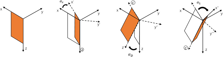
FIGURE 1. Schematic diagram of Euler rotation (Pek and Santos, 2002).

2.2 Vector-scalar-position governing equations based on coulomb gauge

According to the relationship between magnetic vector potential and electric scalar potential (Biro and Preis, 1989)

$\mathbf{B}=\nabla \times \mathbf{A}(8)$

$\mathbf{E}=\mathrm{i}\omega \mathbf{A}-\nabla \mathrm{\Phi }(9)$

Substituting Eqs 8–9 into Eqs 1–2, and introducing the vector identity $\nabla \times \left(\nabla \times \mathbf{A}\right)=\nabla \left(\nabla \cdot \mathbf{A}\right)-{\nabla }^2\mathbf{A}$ and the Coulomb gauge $\nabla \cdot \mathbf{A}=0$ (Everett and Schultz, 1996), we can get the coupled equations of vector potential and scalar potential equations (LaBrecque et al., 1999; Haber et al., 2000; Varilsuha and Candansayar, 2018)

$\left\{\begin{array}{l}{\nabla }^2\mathbf{A}+{\mathit{k}}^2\mathbf{A}-{\mu }_0\mathit{\sigma }\nabla \mathrm{\Phi }=0\\ \nabla \cdot \left(\mathit{\sigma }\nabla \mathrm{\Phi }\right)-\mathrm{i}\omega \nabla \cdot \left(\mathit{\sigma }\mathbf{A}\right)=0\end{array}\right.(10)$

The equations are relatively complete in theory, and the physical meaning is relatively clear, and at this time, the vector position and the scalar position have unique solutions.

Vector potential and scalar potential based on the Coulomb gauge are expressed as

$\left\{\begin{array}{l}\mathbf{A}={\mathbf{A}}^{\mathbf{p}}+{\mathbf{A}}^{\mathbf{s}}\\ \mathrm{\Phi }={\mathrm{\Phi }}^{\mathbf{p}}+{\mathrm{\Phi }}^{\mathbf{s}}\end{array}\right.(11)$

where ${\mathbf{A}}^{\mathbf{p}},{\mathbf{A}}^{\mathbf{s}}$ are the vector potential of the primary field and the vector potential of the secondary field, and ${\mathrm{\Phi }}^{\mathbf{p}},{\mathrm{\Phi }}^{\mathbf{s}}$ are the scalar potential of the primary field and the scalar potential of the secondary field, respectively.

$\left\{\begin{array}{l}{\mathit{k}}^2={\mathit{k}}_p^2+{\mathit{k}}_s^2\\ \mathit{\sigma }={\mathit{\sigma }}_p+{\mathit{\sigma }}_s\end{array}\right.(12)$

where ${\mathit{k}}_p^2$ is the product of the admittance tensor and resistivity corresponding to the primary field, ${\mathit{\sigma }}_p$ is the conductivity tensor corresponding to the primary field, ${\mathit{k}}_s^2$ is the product of the admittance tensor and resistivity corresponding to the secondary field and ${\mathit{\sigma }}_s$ is the conductivity corresponding to the secondary field rate tensor. According to the principle of superposition, the coupling equations satisfied by the secondary field vector potential and scalar potential are

$\left\{\begin{array}{l}{\nabla }^2{\mathbf{A}}^{\mathbf{s}}+{\mathit{k}}_p^2{\mathbf{A}}^{\mathbf{s}}-{\mu }_0{\mathit{\sigma }}_p\nabla {\mathrm{\Phi }}^{\mathbf{s}}=-{\mu }_0{\mathit{\sigma }}_s\mathbf{E}\\ \nabla \cdot \left({\mathit{\sigma }}_p\nabla {\mathrm{\Phi }}^{\mathbf{s}}\right)-\mathrm{i}\omega \nabla \cdot \left({\mathit{\sigma }}_p{\mathbf{A}}^{\mathbf{s}}\right)=\nabla \cdot \left({\mathit{\sigma }}_s\mathbf{E}\right)\end{array}\right.(13)$

Many scholars (Haber et al., 2000; Badea et al., 2001; Jahandari and Farquharson, 2015) used numerical methods to solve the above Eq. 10 or (13) and achieved good results. However, the conventional numerical methods require a large amount of calculation and storage due to the large sparse matrix linear equations (Varilsuha and Candansayar, 2018), especially for any anisotropic medium. In order to decrease the computation and storage load, how to solve the governing equations of vector potential and scalar potential is particularly important. This paper intends to use a rapid 3D numerical simulation method in the Fourier domain (Dai et al., 2022), and this method performs a 2D Fourier transform of Equation 13 along the horizontal directions, a 3D partial differential equation in the space domain is transformed into multiple 1D coupled ordinary differential equations in the Fourier domain, and the coupling between different wave numbers’ ordinary differential equations are independent of each other and have a high degree of parallelism.

2.3 Vector and scalar potential ordinary differential equation in fourier domain

We wrote formula (13) in component form and expanded

$\left\{\begin{array}{c}\frac{{\partial }^2{A}_x^s}{\partial x^2}+\frac{{\partial }^2{A}_x^s}{\partial y^2}+\frac{{\partial }^2{A}_x^s}{\partial z^2}+{\mathit{k}}_p^2{A}_x^s-{\mu }_0{\widehat{\mathit{y}}}_p\frac{\partial {\mathrm{\Phi }}^s}{\partial x}=-{\mu }_0{\mathit{j}}_x^s\\ \frac{{\partial }^2{A}_y^s}{\partial x^2}+\frac{{\partial }^2{A}_y^s}{\partial y^2}+\frac{{\partial }^2{A}_y^s}{\partial z^2}+{\mathit{k}}_p^2{A}_y^s-{\mu }_0{\widehat{\mathit{y}}}_p\frac{\partial {\mathrm{\Phi }}^s}{\partial y}=-{\mu }_0{\mathit{j}}_y^s\\ \frac{{\partial }^2{A}_z^s}{\partial x^2}+\frac{{\partial }^2{A}_z^s}{\partial y^2}+\frac{{\partial }^2{A}_z^s}{\partial z^2}+{\mathit{k}}_p^2{A}_z^s-{\mu }_0{\widehat{\mathit{y}}}_p\frac{\partial {\mathrm{\Phi }}^s}{\partial z}=-{\mu }_0{\mathit{j}}_z^s\\ \begin{array}{l}{\widehat{\mathit{y}}}_p\left(\frac{{\partial }^2{\mathrm{\Phi }}^s}{\partial x^2}+\frac{{\partial }^2{\mathrm{\Phi }}^s}{\partial y^2}+\frac{{\partial }^2{\mathrm{\Phi }}^s}{\partial z^2}\right)+\frac{\partial {\mathrm{\Phi }}^s}{\partial z}\frac{\partial {\widehat{\mathit{y}}}_p}{\partial z}-\mathrm{i}\omega A_z^s\frac{\partial {\widehat{\mathit{y}}}_p}{\partial z}\\ =\frac{\partial {\mathit{j}}_x^s}{\partial x}+\frac{\partial {\mathit{j}}_y^s}{\partial y}+\frac{\partial {\mathit{j}}_z^s}{\partial z}\end{array}\end{array}\right.(14)$

where $A_x^s$, $A_y^s$ and $A_z^s$ are the three components of the secondary field vector potential, ${\mathit{j}}_x^s={\widehat{\mathit{y}}}_s{E}_x^0$, ${\mathit{j}}_y^s={\widehat{\mathit{y}}}_s{E}_y^0$, ${\mathit{j}}_z^s={\widehat{\mathit{y}}}_s{E}_z^0$ are the current density tensors, and $E_x^0$, $E_y^0$ and $E_z^0$ are the background fields.

For formula (14), a 2D Fourier transform is used along the x and y direction

$\left\{\begin{array}{l}\frac{{\partial }^2{\stackrel{\sim }{A}}_x^s}{\partial z^2}+\left({\mathit{k}}_p^2-k_x^2-k_y^2\right){\stackrel{\sim }{A}}_x^s+\mathrm{i}{k}_x{\mu }_0{\widehat{\mathit{y}}}_p{\stackrel{\sim }{\mathrm{\Phi }}}^s=-{\mu }_0{\stackrel{\sim }{\mathit{j}}}_x^s\\ \frac{{\partial }^2{\stackrel{\sim }{A}}_y^s}{\partial z^2}+\left({\mathit{k}}_p^2-k_x^2-k_y^2\right){\stackrel{\sim }{A}}_y^s+\mathrm{i}{k}_y{\mu }_0{\widehat{\mathit{y}}}_p{\stackrel{\sim }{\mathrm{\Phi }}}^s=-{\mu }_0{\stackrel{\sim }{\mathit{j}}}_y^s\\ \frac{{\partial }^2{\stackrel{\sim }{A}}_z^s}{\partial z^2}+\left({\mathit{k}}_p^2-k_x^2-k_y^2\right){\stackrel{\sim }{A}}_z^s-{\widehat{\mathit{y}}}_p{\mu }_0\frac{\partial {\stackrel{\sim }{\mathrm{\Phi }}}^s}{\partial z}=-{\mu }_0{\stackrel{\sim }{\mathit{j}}}_z^s\\ \left({\widehat{\mathit{y}}}_p\frac{{\partial }^2{\stackrel{\sim }{\mathrm{\Phi }}}^s}{\partial z^2}+\frac{\partial {\widehat{\mathit{y}}}_p}{\partial z}\frac{\partial {\stackrel{\sim }{\mathrm{\Phi }}}^s}{\partial z}-{\widehat{\mathit{y}}}_p\left(k_x^2+k_y^2\right){\stackrel{\sim }{\mathrm{\Phi }}}^s\right)+\\ \mathrm{i}\omega \left(\mathrm{i}{k}_x{\widehat{\mathit{y}}}_p{\stackrel{\sim }{A}}_x^s+\mathrm{i}{k}_y{\widehat{\mathit{y}}}_p{A}_y^s-{\widehat{\mathit{y}}}_p\frac{\partial {\stackrel{\sim }{A}}_z^s}{\partial z}\right)-\mathrm{i}\omega {\stackrel{\sim }{A}}_z^s\frac{\partial {\widehat{\mathit{y}}}_p}{\partial z}\\ =-\mathrm{i}{k}_x{\stackrel{\sim }{\mathit{j}}}_x^s-\mathrm{i}{k}_y{\stackrel{\sim }{\mathit{j}}}_y^s+\frac{\partial {\stackrel{\sim }{\mathit{j}}}_z^s}{\partial z}\end{array}\right.(15)$

where $k_x$ and $k_y$ are the wavenumbers in the space wavenumber domain, ${\stackrel{\sim }{A}}_x^s$, ${\stackrel{\sim }{A}}_y^s$ and ${\stackrel{\sim }{A}}_z^s$ are the three components of the secondary field vector potential in the Fourier domain, and ${\stackrel{\sim }{\mathrm{\Phi }}}^s$ are the secondary field scalar potential in the Fourier domain, ${\stackrel{\sim }{\mathit{j}}}_x^s$, ${\stackrel{\sim }{\mathit{j}}}_y^s$ and ${\stackrel{\sim }{\mathit{j}}}_z^s$ are the current densities in the Fourier domain, respectively.

Using a 2D Fourier transform to transform the 3D partial differential coupling Eq. 14 into 1D ordinary differential coupling Eq. 15, thus decomposing a super-large-scale problem into multiple small problems and greatly reducing the anisotropy Medium simulation requires computing time and storage, and the ordinary differential equations between different wave numbers are independent of each other, which has a high degree of parallelism.

2.4 Boundary conditions

In a homogeneous medium, according to the Helmholtz equation and the Coulomb gauge $\nabla \cdot \mathbf{A}=0$ satisfied by the electric field vector $\mathbf{E}$, combined with the relationship between the vector potential $\mathbf{A}$, the scalar potential $\mathrm{\Phi }$ and the electromagnetic field, and the lower and upper boundary conditions of the vector potential $\stackrel{\sim }{\mathbf{A}}$ , scalar potential $\stackrel{\sim }{\mathrm{\Phi }}$ in the Fourier domain can be obtained

$\left\{\begin{array}{l}\frac{\partial {\stackrel{\sim }{A}}_x^s}{\partial z}=-s{\stackrel{\sim }{A}}_x^s+\frac{\left(t-s\right)}{\omega }{k}_x{\stackrel{\sim }{\mathrm{\Phi }}}^s\\ \frac{\partial {\stackrel{\sim }{A}}_y^s}{\partial z}=-s{\stackrel{\sim }{A}}_y^s+\frac{\left(t-s\right)}{\omega }{k}_y{\stackrel{\sim }{\mathrm{\Phi }}}^s\\ \frac{\partial {\stackrel{\sim }{A}}_z^s}{\partial z}=\mathrm{i}{k}_x{\stackrel{\sim }{A}}_x^s+\mathrm{i}{k}_y{\stackrel{\sim }{A}}_y^s\\ \frac{\partial {\stackrel{\sim }{\mathrm{\Phi }}}^s}{\partial z}=-t{\stackrel{\sim }{\mathrm{\Phi }}}^s\end{array}\right.(16)$

$\left\{\begin{array}{l}\frac{\partial {\stackrel{\sim }{A}}_x^s}{\partial z}=s{\stackrel{\sim }{A}}_x^s-\mathrm{i}{k}_x{\stackrel{\sim }{A}}_z^s+\frac{s{k}_x{\stackrel{\sim }{\mathrm{\Phi }}}^s}{\omega }\\ \frac{\partial {\stackrel{\sim }{A}}_y^s}{\partial z}=s{\stackrel{\sim }{A}}_y^s-\mathrm{i}{k}_y{\stackrel{\sim }{A}}_z^s+\frac{s{k}_y{\stackrel{\sim }{\mathrm{\Phi }}}^s}{\omega }\\ \frac{\partial {\stackrel{\sim }{A}}_z^s}{\partial z}=\mathrm{i}{k}_x{\stackrel{\sim }{A}}_x^s+\mathrm{i}{k}_y{\stackrel{\sim }{A}}_y^s\\ \frac{\partial {\stackrel{\sim }{\mathrm{\Phi }}}^s}{\partial z}=\mathrm{i}\omega {\stackrel{\sim }{A}}_z^s\end{array}\right.(17)$

2.5 Finite element method

Eq. 15 is the coupled ordinary differential equation satisfied by the vector and scalar potentials in the Fourier domain, and Eqs 16, 17 are the lower and upper boundary conditions, respectively. For Eqs 15–17 boundary value problems, this paper intends to use the one-dimensional finite element method based on quadratic interpolation to solve them. Using the Galerkin method to transform the boundary value problem of Eqs 15–17 into finite element equations

$\left\{\begin{array}{l}{\displaystyle \sum _{e=1}^{Ne}}{\int }_e\left(-\frac{\partial {\stackrel{\sim }{A}}_x^s}{\partial z}\frac{\partial N_i}{\partial z}+\left({\mathit{k}}_p^2-k_x^2-k_y^2\right)N_i{\stackrel{\sim }{A}}_x^s+\mathrm{i}{k}_x{\mu }_0{\mathit{\sigma }}_p{N}_i{\stackrel{\sim }{\mathrm{\Phi }}}^s+N_i{\mu }_0{\stackrel{\sim }{\mathit{j}}}_x^s\right)\mathrm{d}\mathrm{z}\\ +{\displaystyle \sum _{e=1}^{Ne}}{\int }_s{N}_i\frac{\partial {\stackrel{\sim }{A}}_x^s}{\partial z}{n}_z\mathrm{d}\mathrm{z}=0\\ {\displaystyle \sum _{e=1}^{Ne}}{\int }_e\left(-\frac{\partial {\stackrel{\sim }{A}}_y^s}{\partial z}\frac{\partial N_i}{\partial z}+\left({\mathit{k}}_p^2-k_x^2-k_y^2\right)N_i{\stackrel{\sim }{A}}_y^s+\mathrm{i}{k}_y{\mu }_0{\mathit{\sigma }}_p{N}_i{\stackrel{\sim }{\mathrm{\Phi }}}^s+N_i{\mu }_0{\stackrel{\sim }{\mathit{j}}}_y^s\right)\mathrm{d}\mathrm{z}\\ +{\displaystyle \sum _{e=1}^{Ne}}{\int }_s{N}_i\frac{\partial {\stackrel{\sim }{A}}_y^s}{\partial z}{n}_z\mathrm{d}\mathrm{z}=0\\ {\displaystyle \sum _{e=1}^{Ne}}{\int }_e\left(-\frac{\partial {\stackrel{\sim }{A}}_z^s}{\partial z}\frac{\partial N_i}{\partial z}+\left({\mathit{k}}_p^2-k_x^2-k_y^2\right)N_i{\stackrel{\sim }{A}}_z^s-{\mu }_0{\mathit{\sigma }}_p{N}_i\frac{\partial {\stackrel{\sim }{\mathrm{\Phi }}}^s}{\partial z}+N_i{\mu }_0{\stackrel{\sim }{\mathit{j}}}_z^s\right)\mathrm{d}\mathrm{z}\\ +{\displaystyle \sum _{e=1}^{Ne}}{\int }_s{N}_i\frac{\partial {\stackrel{\sim }{A}}_z^s}{\partial z}{n}_z\mathrm{d}\mathrm{z}=0\\ {\displaystyle \sum _{e=1}^{Ne}}{\int }_e\left(-{\mathit{\sigma }}_p\frac{\partial {\stackrel{\sim }{\mathrm{\Phi }}}^s}{\partial z}\frac{\partial N_i}{\partial z}+N_i\frac{\partial {\widehat{\mathit{y}}}_p}{\partial z}\frac{\partial {\stackrel{\sim }{\mathrm{\Phi }}}^s}{\partial z}-{\mathit{\sigma }}_p\left(k_x^2+k_y^2\right)N_i{\stackrel{\sim }{\mathrm{\Phi }}}^s\right)\mathrm{d}\mathrm{z}+\\ {\displaystyle \sum _{e=1}^{Ne}}{\int }_e\left(-\mathrm{i}\omega N_i\frac{\partial {\widehat{\mathit{y}}}_p}{\partial z}{\stackrel{\sim }{A}}_z^s+\mathrm{i}{k}_x{N}_i{\stackrel{\sim }{\mathit{j}}}_x^s+\mathrm{i}{k}_y{N}_i{\stackrel{\sim }{\mathit{j}}}_y^s-N_i\frac{\partial {\stackrel{\sim }{\mathit{j}}}_z^s}{\partial z}\right)\mathrm{d}\mathrm{z}+\\ {\displaystyle \sum _{e=1}^{Ne}}{\int }_s{\mathit{\sigma }}_p{N}_i\frac{\partial {\stackrel{\sim }{\mathrm{\Phi }}}^s}{\partial z}{n}_z\mathrm{d}\mathrm{z}=0\end{array}\right.(18)$

where $Ne$ is the number of vertical unit subdivisions, $N_i\left(i=j,p,m\right)$ is the quadratic interpolation function of the eth unit and the ith node (Xu, 1994). For Eq. 18, there are mainly seven types of integrals (Dai et al., 2022); the overall synthesis of each unit integral can be obtained as a diagonal equation system with a bandwidth of 23

$\mathbf{K}\mathbf{u}=\mathbf{P}(19)$

where $\mathbf{K}$ is a 23-diagonal matrix, $\mathbf{P}$ is the source term, and $\mathbf{u}$ is the Fourier domain vector and scalar potential to be obtained. Linear Eq. 19 can be quickly solved using the chasing method. The numerical simulation method adopted in this paper transforms the 3D problem into multiple independent 1D problems, which fundamentally change the characteristics and solution methods of the governing equation. Compared with the iterative solution method and the direct solution method, the pursuit method has the advantage of solving ordinary differential equations; its high parallelism greatly reduces the simulation time and memory consumption.

The other components of the electromagnetic field in the Fourier domain can be obtained through the relationship between the magnetic vector potential and the electric scalar potential and the electromagnetic field (8)∼(9). The electromagnetic field in the space domain can be obtained by the 2D inverse Fourier transform of the electromagnetic field in the Fourier domain (Dai et al., 2022).

2.6 Compact operator iteration scheme

For the above formula (18), the solution obtained by the finite element method is the Born approximate solution, and it is difficult to achieve stable convergence or even divergence by direct iteration. For the convergence problem, here, the scalar iteration format for stable convergence in isotropic media is extended as tensor form (Gao, 2005; Dai et al., 2022).

${\mathbf{E}}^{\left(n\right)}=\mathbf{\alpha }{\mathbf{E}}^{\left(n\right)}+\mathbf{\beta }{\mathbf{E}}^{\left(n-1\right)}(20)$

where $\mathbf{\alpha },\mathbf{\beta }$ is the tensor related to the background field conductivity ${\mathit{\sigma }}_b$ , the difference $\Delta \mathit{\sigma }$ between the abnormal bulk conductivity and the background field conductivity is calculated as follows:

$\mathbf{\alpha }=\frac{2{\mathit{\sigma }}_b}{2{\mathit{\sigma }}_b+\mathbf{\Delta }\mathit{\sigma }}(21)$

$\mathbf{\beta }=\frac{\mathbf{\Delta }\mathit{\sigma }}{2{\mathit{\sigma }}_b+\mathbf{\Delta }\mathit{\sigma }}(22)$

2.7 Apparent resistivity and phase

Assuming that the ground electromagnetic fields excited by two linearly independent field sources are $E_{x1}$, $E_{y1}$, $H_{x1}$, $H_{y1}$ and $E_{x2}$, $E_{y2}$, $H_{x2}$, $H_{y2}$, respectively, the impedance tensors of XX, XY, YX, and YY polarization modes can be obtained.

$Z_{xx}=\frac{E_{x1}{H}_{y2}-E_{x2}{H}_{y1}}{H_{x1}{H}_{y2}-H_{x2}{H}_{y1}}(23)$

$Z_{xY}=\frac{E_{x2}{H}_{x1}-E_{x1}{H}_{x2}}{H_{x1}{H}_{y2}-H_{x2}{H}_{y1}}(24)$

$Z_{yx}=\frac{E_{y1}{H}_{y2}-E_{y2}{H}_{y1}}{H_{x1}{H}_{y2}-H_{x2}{H}_{y1}}(25)$

$Z_{yy}=\frac{E_{y2}{H}_{x1}-E_{y1}{H}_{x2}}{H_{x1}{H}_{y2}-H_{x2}{H}_{y1}}(26)$

Then, according to the apparent resistivity and phase formulas, we can get

${\rho }_{ij}=\frac{{\left|Z_{ij}\right|}^2}{\omega \mu },{\phi }_{ij}=\arg \left(Z_{ij}\right)\left(i,j=x,y\right)(27)$

3 Numerical experiments

3.1 Calculation accuracy and time-consuming comparison

In order to verify the accuracy of the algorithm proposed in this paper, the one-dimensional anisotropic medium model in the article by Rasmussen (1988) was used to compare the calculation results. This one-dimensional model was used as a test model by Pek and Santos (2002) and Han et al. (2018). The model is divided into four layers: the second and third layers are anisotropic media and the first and bottom layers are isotropic media (Figure 2). The first layer of the model has a resistivity of 10000Ω⋅m and a thickness of 10km; the depths of the second and third layers are 18 km and 100 km, respectively, and the principal axis resistivity is 200/20000/200Ω⋅m and 1000/2000/1000Ω⋅m, respectively; the Euler rotation angle α_s is 15° and −75°, respectively, and the angles α_d and α_l are both zero. The bottom layer is an isotropic medium with a resistivity of 100Ω⋅m.

FIGURE 2

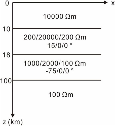
FIGURE 2. Schematic diagram of the 1D model.

The number of grid nodes calculated by our algorithm is 101×101×81, and the number of air layers is set to 10. The frequency used in the forward modeling is 31 frequency points taken at logarithmic intervals from 0.0001 Hz to 100 Hz. The calculated numerical solution is compared with the one-dimensional analytical solution given by Pek and Santos (2002) (Figure 3). The relative error and phase error of apparent resistivity are calculated, as shown in Figure 4. It can be seen that the relative error of apparent resistivity is less than 1%, and the error of phase is less than 0.2°. Therefore, the calculation accuracy of this algorithm satisfies the requirements of magnetotelluric simulation.

FIGURE 3

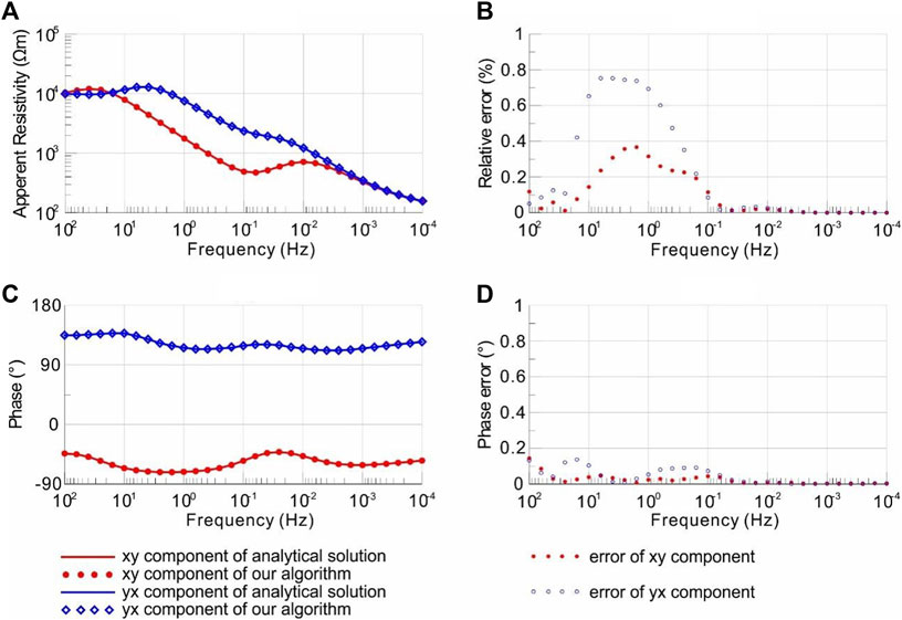
FIGURE 3. Comparison of apparent resistivity and phase calculation results. (A) Apparent resistivity, (B) phase, (C) relative error of apparent resistivity, and (D) error of phase.

FIGURE 4

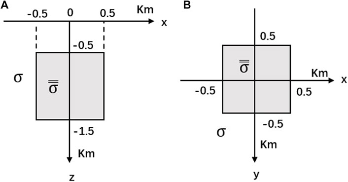
FIGURE 4. 3D land anisotropy model: (A) section view along the x-axis and (B) plan view.

The 3D numerical simulation algorithm in this paper has the feature of high parallelism, and its calculation time and memory cost will not increase exponentially with the number of mesh nodes but will increase approximately linearly. This feature is suitable for the numerical simulation of large-scale complex 3D models.

The algorithms in this paper are written in Fortran 95 language, and the calculation platform is Intel(R) Xeon(R) CPU3.1G, 64GB RAM, 16CPUs, which is basically the same configuration as in Zhang et al. (2017). According to the 3D model by Zhang et al. (2017), we design a model with a mesh number of 119×65×38 (the grid nodes number is 120×66×39) to test the calculation efficiency and memory usage of the algorithm in this paper.

Zhang et al. (2017) used four algorithms: 1) algorithm based on total field finite element (TFE); 2) algorithm based on secondary field finite element (SFE); 3) algorithm based on total field finite element and infinite element (TFEIE); 4) algorithm based on the secondary field finite-element and infinite element (SFEIE). The SFE and TFE algorithms adopt the truncated boundary condition, and the electric field on the boundary is assumed to be zero, so a larger calculation area (57.2×56.8×40 km³) is needed, while a smaller calculation area (6×6×4 km³) can be set for the SFEIE and TFEIE algorithms. For comparison, we also designed a model with a larger calculation area (57.2×56.8×40 km³), and the grid nodes number is 256×256×151. Table 1 lists the calculation memory and calculation time of the algorithm in this paper (MSWD) and the four algorithms of Zhang et al. (2017).

TABLE 1

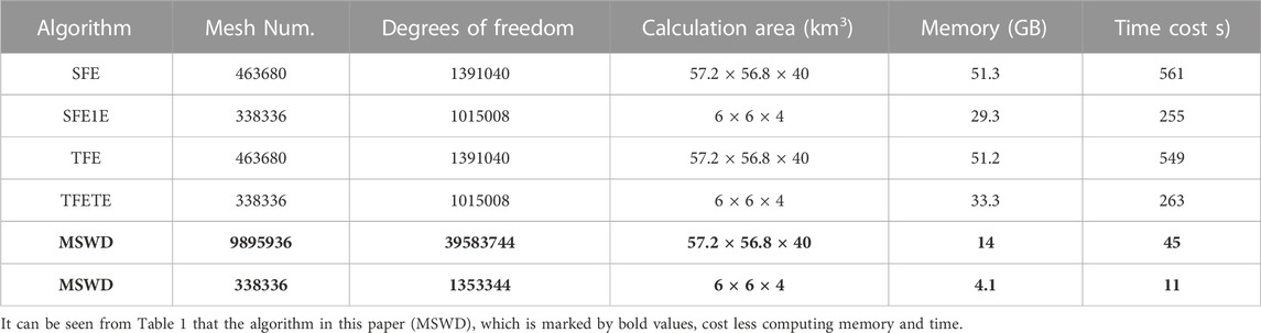
TABLE 1. The comparison of the memory and time obtained with the five algorithms.

The algorithm (MSWD) proposed in this paper has a high degree of parallelism, and its forward modeling speed is 1–2 orders of magnitude faster than the traditional finite element method, and it consumes less memory.

The calculation advantage of the algorithm (MSWD) in this paper is more obvious in the model with numerous meshes.

3.2 The 3D anisotropic land model

Referring to the model by Xiao et al. (2019), an anisotropic 3D anomalous body model with a size of 1 km × 1 km × 1 km was selected as shown in Figure 4, in which the top surface of the anomalous body is 0.5 km away from the surface. For comparison, the surrounding rock around the abnormal body is set as an isotropic medium with a resistivity of 100 Ωm.

First of all, we studied the horizontal anisotropy, and the main axis resistivity of the 3D anisotropic anomalous body is taken as 1000, 10, and 100, the Euler rotation angle α_d and α_l are 0°, and the angle α_s is taken as 0°, 30°, 60°, and 90°. In this paper, the cuboid unit is used to divide the grid of the research area, and a total of 96×96×80 (97×97×81 grid nodes) grid units are discretized, and the number of air layers is five. The forward modeling result of the finite element method at a frequency of 0.1 Hz is shown in Figure 5.

FIGURE 5

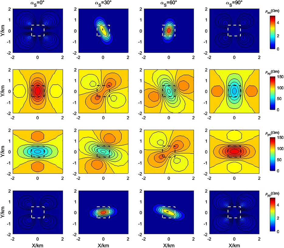
FIGURE 5. Apparent resistivity plan at different strike angles at 0.1Hz.

Figure 5 contains 16 sub-figures; from left to right are the results of taking the α_s values of 0°, 30°, 60°, and 90°, and from top to bottom are the apparent resistivity of XX mode, XY mode, YX mode, and YY mode. These figures show that when α_s=0°, the apparent resistivity of the XY mode at the abnormal body position mainly depends on the spindle resistivity ρ_x, and the apparent resistivity of the YX mode at the abnormal body position depends on the spindle resistivity ρ_y. With the change of α_s, the apparent resistivity changes of XY mode and YX mode also rotate accordingly. When α_s=90°, the apparent resistivity of the XY mode at the abnormal body position is mainly related to the spindle resistivity ρ_y, and the apparent resistivity of the YX mode at the abnormal body position is related to the spindle resistivity ρ_x. It shows that when the main axis resistivity is constant and the α_s changes, the apparent resistivity of both the XY mode and YX mode changes, and the directionality of apparent resistivity imaging is related to the α_s.

We then studied the tilt anisotropy, and the 3D anomalous body model is the same as above; the main axis resistivity is still 1000, 10, and 100; however, this time, the Euler rotation angle sum is 0°, and the Euler rotation angle is 0°, 30°, 60°, and 90°. The calculation frequency is also 0.1Hz, and the forward simulation results are shown in Figure 6.

FIGURE 6

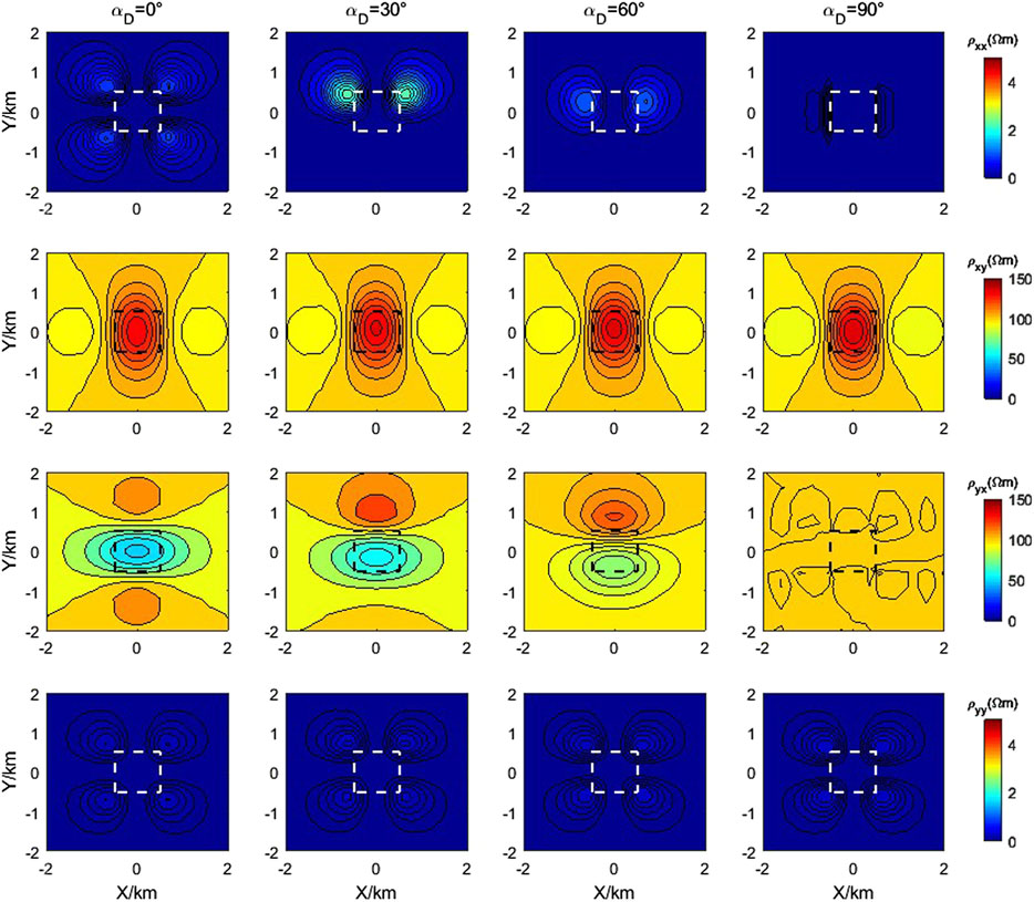
FIGURE 6. Apparent resistivity plan at different angles ${\mathit{\alpha }}_{\mathit{D}}$ at 0.1Hz.

Figure 6 includes 16 subgraphs, which are arranged in the same way as mentioned above. From the apparent resistivity imaging in the figure, it can be seen that no matter how the Euler rotation angle α_d changes, the apparent resistivity ρ_xy does not change. This is because the Euler rotation angle α_d changes around the x-axis, so the resistivity ρ_x of the anomaly position does not change, indicating that the apparent resistivity ρ_xy is only related to the principal axis resistivity ρ_x. However, the apparent resistivity ρ_yx changes with the change in the Euler rotation angle. When the Euler rotation angle α_d = 90°, the resistivity in the y direction of the abnormal body position is 10. At this time, a large low-resistance anomaly appears at the abnormal body position. When the Euler rotation angle is applied, the resistivity of the abnormal body position in the y direction is equal to the principle axis resistivity ρ_z which is 100. At this time, the apparent resistivity of the abnormal body position is almost consistent with the surrounding rock area within the allowable range of error, which is also the main axis anisotropic; the off-diagonal elements of the anisotropic conductivity tensor matrix are zero. When the Euler rotation angle α_d changes from 0° to 90°, the apparent resistivity near the position of the abnormal body increases, since the principal axis resistivity is ρ_z is larger than ρ_y, this means the component in the y direction is related to the principal axis resistivity ρ_y and ρ_z. In addition, the apparent resistivity imaging of the XX mode and YY mode shows that the apparent resistivity change of XX mode is related to YX mode when the tilt anisotropy occurs, and the imaging of YY mode is similar to that of XY mode.

3.3 3D anisotropy ocean model

In order to verify the influence of resistivity anisotropy on the magnetotelluric response in the seabed model, this paper improves the marine oil and gas reservoir model designed by Li and Dai (2011) with resistivity anisotropy of surrounding rock, as shown in Figure 7. The air resistivity is 10⁸Ωm; the resistivity of seawater is 0.3Ωm, and the thickness of seawater is 1000 m; the seabed is the anisotropic medium, and an isotropic high-resistivity oil and gas reservoir exists at 1000 m below the seabed, with a resistivity of 50Ωm; the length and width are 6000 m, and the thickness is 100 m. The research frequency is 0.25Hz, and the electromagnetic-receiving devices are placed on the seabed −14 km–14 km.

FIGURE 7

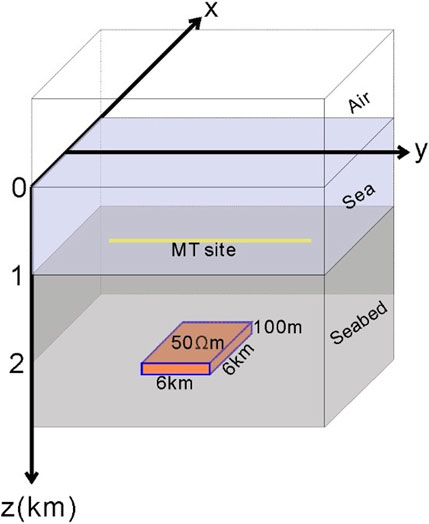
FIGURE 7. Schematic diagram of 3D anisotropic ocean model.

3.3.1 Influence of ${\rho }_x$

In the resistivity anisotropic medium model shown in Figure 7, it is assumed that ${\rho }_y={\rho }_z=1.0\mathrm{\Omega }\mathrm{m}$ in the anisotropic medium layer is constant, and its influence on the electromagnetic response is studied by changing the resistivity of the main coordinate axis ${\rho }_x$ as $1\mathrm{\Omega }\mathrm{m}$, $2\mathrm{\Omega }\mathrm{m}$, $4\mathrm{\Omega }\mathrm{m}$, and $10\mathrm{\Omega }\mathrm{m}$. The calculation results are shown in Figure 8. From the calculation results, it can be seen that the influence of ${\rho }_x$ on the xy component of the apparent resistivity is more obvious than that of the yx component.

FIGURE 8

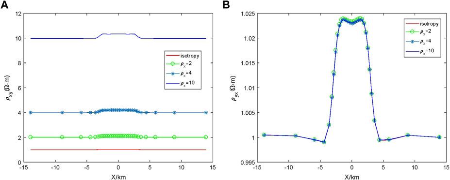
FIGURE 8. Effect of ${\rho }_x$ on apparent resistivity: (A) xy component and (B) yx component.

3.3.2 Influence of ${\rho }_y$

In the anisotropic resistivity medium model shown in Figure 7, it is assumed that the resistivity of the principal axis of the anisotropic medium layer ${\rho }_x={\rho }_z=1.0\mathrm{\Omega }\mathrm{m}$ remains unchanged, and the effect of the resistivity of the principal coordinate axis on the electromagnetic response is studied by changing the resistivity of the principal coordinate axis ${\rho }_y$ as $1\mathrm{\Omega }\mathrm{m}$, $2\mathrm{\Omega }\mathrm{m}$, $4\mathrm{\Omega }\mathrm{m}$, and $10\mathrm{\Omega }\mathrm{m}$. The calculation results are shown in Figure 9. From the calculation results, it can be seen that the influence of ${\rho }_y$ on the yx component of the apparent resistivity is more obvious than the xy component.

FIGURE 9

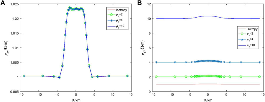
FIGURE 9. Effect of ${\rho }_y$ on apparent resistivity: (A) xy component and (B) yx component.

3.3.3 Influence of ${\rho }_z$

In the anisotropic resistivity medium model shown in Figure 7, it is assumed that the resistivity of the principal axis of the anisotropic medium layer ${\rho }_x={\rho }_y=1.0\mathrm{\Omega }\mathrm{m}$ remains unchanged, and the effect of the resistivity of the principal coordinate axis on the electromagnetic response is studied by changing the resistivity of the principal coordinate axis ${\rho }_z$ as $1\mathrm{\Omega }\mathrm{m}$, $2\mathrm{\Omega }\mathrm{m}$, $4\mathrm{\Omega }\mathrm{m}$, and $10\mathrm{\Omega }\mathrm{m}$. The calculation results are shown in Figure 10. From the calculation results, it can be seen that ${\rho }_z$ has an influence on both the xy component and the yx component of the apparent resistivity. Relatively speaking, the influence range of the xy component is larger than that of the yx component.

FIGURE 10

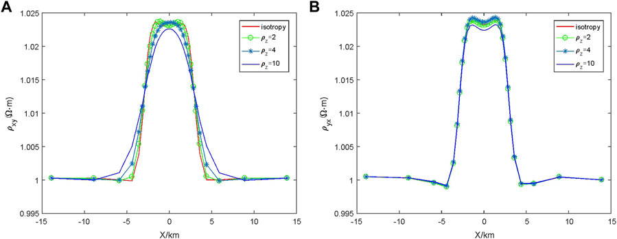
FIGURE 10. Effect of ${\rho }_z$ on apparent resistivity: (A) xy component and (B) yx component.

3.3.4 Influence of ${\alpha }_d$

In the resistivity anisotropic medium model shown in Figure 7, it is assumed that the resistivity of the principal axis of the anisotropic dielectric layer is ${\rho }_x={\rho }_y=1.0\mathrm{\Omega }\mathrm{m}$ and ${\rho }_z=4\mathrm{\Omega }\mathrm{m}$ ; the effect on the electromagnetic response is studied by changing the anisotropic dip angle ${\alpha }_d$ as 0°, 30°, 45°, 60°, and 90°. According to the different angles of anisotropy, it can be divided into three types. When ${\alpha }_d=0^{。}$, it is called transverse isotropy vertical (TIH); when ${\alpha }_d$ =30°, 45°, and 60°, it is called transverse isotropy dip (TID); when ${\alpha }_d={90}^{。}$, it is called transverse isotropy horizontal (TIV). The calculation results are shown in Figure 11. From the calculation results, we can see that ${\alpha }_d$ has an influence on both the xy component and the yx component of the apparent resistivity. Relatively, the influence range of the xy component is larger than that of the yx component.

FIGURE 11

FIGURE 11. Effect of ${\alpha }_d$ on apparent resistivity: (A) xy component and (B) yx component.

3.3.5 Influence of ${\alpha }_s$

In the resistivity anisotropic medium model shown in Figure 7, it is assumed that the resistivity of the principal axis of the anisotropic layer is ${\rho }_x=4\mathrm{\Omega }\mathrm{m}$ and ${\rho }_y={\rho }_z=1.0\mathrm{\Omega }\mathrm{m}$; the effect on the electromagnetic response is studied by changing the anisotropic strike angle ${\alpha }_s$ as 0°, 30°, 45°, 60°, and 90°. The calculation results are shown in Figure 12. From the calculation results, it can be seen that ${\alpha }_s$ has a greater influence on the yx component of the apparent resistivity than the xy component.

FIGURE 12

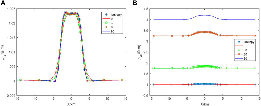
FIGURE 12. Effect of ${\alpha }_s$ on apparent resistivity: (A) xy component and (B) yx component.

4 Conclusion

In this paper, from the perspective of improving the calculation efficiency of 3D anisotropic magnetotelluric numerical simulation, a Fourier domain anisotropic 3D magnetotelluric simulation algorithm is proposed. This algorithm transforms the space domain equation into the Fourier domain, reduces the solution dimension, and improves the calculation efficiency. A one-dimensional model is used to test the correctness of the algorithm, and a land model and a group of ocean models are calculated using this algorithm, The influence characteristics of resistivity anisotropy on the magnetotelluric response function in different models are discussed respectively.

Data availability statement

The raw data supporting the conclusion of this article will be made available by the authors, without undue reservation.

Author contributions

YZ did most of the forward method study. GS did most of the data process and analysis work. XW and WZ did the numerical experience work. All authors contributed to the article and approved the submitted version.

Funding

This paper is supported by the 2022-2023 key scientific research project of the Shandong Coalfield Geology Bureau (LUMEIDIKEZI 2022-19; LUMEIDIKEZI 2022-60) and Shandong Provincial Natural Science Foundation (ZR2023QD084).

Conflict of interest

The authors declare that the research was conducted in the absence of any commercial or financial relationships that could be construed as a potential conflict of interest.

Publisher’s note

All claims expressed in this article are solely those of the authors and do not necessarily represent those of their affiliated organizations, or those of the publisher, the editors and the reviewers. Any product that may be evaluated in this article, or claim that may be made by its manufacturer, is not guaranteed or endorsed by the publisher.

References

Andréa, D., and Li, Y. (2022). Understanding the effect of 1-D dipping anisotropic conductivity on the response and interpretation of magnetotelluric data. Geophys. J. Int. 3 (3), 1948–1965. doi:10.1093/gji/ggac166

CrossRef Full Text | Google Scholar

Badea, E. A., Everett, M. E., Newman, G. A., and Biro, O. (2001). Finite element analysis of controlled-source electromagnetic induction using Coulomb-gauged potentials. Geophysics 66 (3), 786–799. doi:10.1190/1.1444968

CrossRef Full Text | Google Scholar

Biro, O., and Preis, K. (1989). On the use of the magnetic vector potential in the finite-element analysis of three-dimensional eddy currents. IEEE Trans. Magnetics 25 (4), 3145–3159. doi:10.1109/20.34388

CrossRef Full Text | Google Scholar

Cao, X., Yin, C., Zhang, B., Huang, X., Liu, Y., and Cai, J. (2018). A goal-oriented adaptive finite-element method for 3D MT anisotropic modeling with topography. Chin. J. Geophys. (in Chinese) 61 (6), 2618–2628. doi:10.6038/cjg2018L0068

CrossRef Full Text | Google Scholar

Dai, S., Li, K., Zhou, Y., and Chen, L. (2019a). “Large-scale 3D forward modeling of magnetic anomaly in a mixed space-wavenumber domain,” in GEM 2019 xi'an: International workshop and gravity, electrical & magnetic methods and their applications, chenghu, China.

CrossRef Full Text | Google Scholar

Dai, S., Ling, J., Chen, Q., Li, K., Zhang, Q., Zhao, D., et al. (2021). Numerical modeling of 3D DC resistivity method in the mixed space-wavenumber domain. Applied Geophysics 18 (3), 361–374. doi:10.1007/s11770-021-0904-4

CrossRef Full Text | Google Scholar

Dai, S., Zhao, D., Wang, S., Li, K., and Jahandari, H. (2022). Three-dimensional magnetotelluric modeling in a mixed space-wavenumber domain. Geophysics 87, E205–E217. doi:10.1190/geo2021-0216.1

CrossRef Full Text | Google Scholar

Dai, S., Zhao, D., Wang, S., Xiong, B., Zhang, Q., Li, K., et al. (2019b). Three-dimensional numerical modeling of gravity and magnetic anomaly in a mixed space-wavenumber domain. Geophysics 84 (4), G41–G54. doi:10.1190/geo2018-0491.1

CrossRef Full Text | Google Scholar

Dai, S., Zhao, D., Zhang, Q., Li, K., Chen, Q., and Wang, X. (2018). Three-dimensional numerical modeling of gravity anomalies based on Poisson equation in space-wavenumber mixed domain. Applied Geophysics 15 (3-4), 513–523. doi:10.1007/s11770-018-0702-9

CrossRef Full Text | Google Scholar

Everett, M., and Schultz, A. (1996). Geomagnetic induction in a heterogenous sphere: azimuthally symmetric test computations and the response of an undulating 660-km discontinuity. Journal of Geophysical Research Solid Earth 101 (B2), 2765–2783. doi:10.1029/95jb03541

CrossRef Full Text | Google Scholar

Gao, G. (2005). Simulation of borehole electromagnetic measurements in dipping and anisotropic rock formations and inversion of array induction data. University of Texas.

Google Scholar

Guo, Z., Egbert, G., Dong, H., and Wei, W. (2020). Modular finite volume approach for 3Dmagnetotelluric modeling of the earth medium with general anisotropy. Physics of the Earth and Planetary Interiors 309, 106585. doi:10.1016/j.pepi.2020.106585

CrossRef Full Text | Google Scholar

Haber, E., Ascher, U., Aruliah, D., and Oldenburg, D. (2000). Fast simulation of 3D electromagnetic problems using potentials. Journal of Computational Physics 163 (1), 150–171. doi:10.1006/jcph.2000.6545

CrossRef Full Text | Google Scholar

Han, B., Li, Y., and Li, G. (2018). 3D forward modeling of magnetotelluric fields in general anisotropic media and its numerical implementation in Julia. Geophysics 83 (4), F29–F40. doi:10.1190/Geo2017-0515.1

CrossRef Full Text | Google Scholar

Jahandari, H., and Farquharson, C. (2015). Finite-volume modelling of geophysical electromagnetic data on unstructured grids using potentials. Geophysical Journal International 202 (3), 1859–1876. doi:10.1093/gji/ggv257

CrossRef Full Text | Google Scholar

Keller, G. (1982). Handbook of physical properties of rocks. Boca Raton: CRC Press, 414. doi:10.1201/9780203712115

CrossRef Full Text | Google Scholar

Kovacikova, S., and Pek, J. (2002). Generalized Riccati equations for 1-D magnetotelluric impedances over anisotropic conductors Part I: plane wave field model. Earth, Planets and Space 54, 473–482. doi:10.1186/bf03353038

CrossRef Full Text | Google Scholar

Labrecque, D., Morelli, G., Daily, W., Ramirez, A., and Lundegard, P. (1999). Occam's inversion of 3-D electrical resistivity tomography. Society of Exploration Geophysicists. doi:10.1190/1.9781560802154.ch37

CrossRef Full Text | Google Scholar

Li, B., Han, T., Fu, L., and Yan, H. (2022). Pressure effects on the anisotropic electrical conductivity of artificial porous rocks with aligned fractures. Geophysical Prospecting 70 (4), 790–800. doi:10.1111/1365-2478.13184

CrossRef Full Text | Google Scholar

Li, G., Wu, S., Cai, H., He, Z., Liu, X., Zhou, C., et al. (2023). IncepTCN: a new deep temporal convolutional network combined with dictionary learning for strong cultural noise elimination of controlled-source electromagnetic data. Geophysics 88 (4), E107–E122. doi:10.1190/geo2022-0317.1

CrossRef Full Text | Google Scholar

Li, Y. (2002). A finite-element algorithm for electromagnetic induction in two-dimensional anisotropic conductivity structures. Geophysical Journal International 148 (3), 389–401. doi:10.1046/j.1365-246x.2002.01570.x

CrossRef Full Text | Google Scholar

Li, Y., and Dai, S. (2011). Finite element modelling of marine controlled-source electromagnetic responses in two-dimensional dipping anisotropic conductivity structures. Geophysical Journal International 185 (2), 622–636. doi:10.1111/j.1365-246X.2011.04974.x

CrossRef Full Text | Google Scholar

Li, Y., and Pek, J. (2008). Adaptive finite element modelling of two-dimensional magnetotelluric fields in general anisotropic media. Geophysical Journal International 175 (3), 942–954. doi:10.1111/j.1365-246X.2008.03955.x

CrossRef Full Text | Google Scholar

Liu, Y., Xu, Z., and Li, Y. (2018). Adaptive finite element modelling of three-dimensional magnetotelluric fields in general anisotropic media. Journal of Applied Geophysics 151, 113–124. doi:10.1016/j.jappgeo.2018.01.012

CrossRef Full Text | Google Scholar

Luo, T., Hu, X., Chen, L., and Xu, G. (2022). Investigating the magnetotelluric responses in electrical anisotropic media. Remote Sensing 14 (10), 2328–2346. doi:10.3390/rs14102328

CrossRef Full Text | Google Scholar

Okazaki, T., Oshiman, N., and Yoshimura, R. (2016). Analytical investigations of the magnetotelluric directionality estimation in 1-D anisotropic layered media. Physics of the Earth and Planetary Interiors 260, 25–31. doi:10.1016/j.pepi.2016.09.002

CrossRef Full Text | Google Scholar

Parkhomenko, E. I. (1967). Electrical properties of rocks. New York: Plenum Press.

Google Scholar

Pek, J., and Santos, F. A. M. (2002). Magnetotelluric impedances and parametric sensitivities for 1-D anisotropic layered media. Computers & Geosciences 28 (28), 939–950. doi:10.1016/s0098-3004(02)00014-6

CrossRef Full Text | Google Scholar

Pek, J., and Verner, T. (1997). Finite-difference modelling of magnetotelluric fields in two-dimensional anisotropic media. Geophys. J. Int. 128, 505–521. doi:10.1111/j.1365-246x.1997.tb05314.x

CrossRef Full Text | Google Scholar

Rasmussen, T. (1988). Magnetotellurics in southwestern Sweden: evidence for electrical anisotropy in the lower crust. Journal of Geophysical Research Solid Earth 93 (B7), 7897–7907. doi:10.1029/JB093iB07p07897

CrossRef Full Text | Google Scholar

Reddy, I. K., and Rankin, D. (1975). Magnetotelluric response of laterally inhomogeneous and anistotropic media. Geophysics 40, 1035–1045. doi:10.1190/1.1440579

CrossRef Full Text | Google Scholar

Rivera-Rios, A. M., Zhou, B., Heinson, G., and Krieger, L. (2019). Multi-order vector finite element modeling of 3D magnetotelluric data including complex geometry and anisotropy. Earth Planets and Space 71 (1), 92–25. doi:10.1186/s40623-019-1071-1

CrossRef Full Text | Google Scholar

Saraf, P. D., Negi, J. G., and Cerv, V. (1986). Magnetotelluric response of a laterally inhomogeneous anisotropic inclusion. Phys. Earth Planet. Inter. 43, 196–198. doi:10.1016/0031-9201(86)90046-4

CrossRef Full Text | Google Scholar

Varilsuha, D., and Candansayar, M. E. (2018). 3D magnetotelluric modeling by using finite-difference method: comparison study of different forward modeling approaches. Geophysics 83 (2), WB51–WB60. doi:10.1190/geo2017-0406.1

CrossRef Full Text | Google Scholar

Weiss, C. J., and Newman, G. A. (2000). Electromagnetic induction in a fully 3D anisotropic Earth. SEG Technical Program Expanded Abstracts, 351–354. doi:10.1190/1.1816064

CrossRef Full Text | Google Scholar

Xiao, T., Huang, X., and Wang, Y. (2019). Three-dimensional magnetotelluric modelling in anisotropic media using the A-phi method. Exploration Geophysics 50 (1), 31–41. doi:10.1080/08123985.2018.1564274

CrossRef Full Text | Google Scholar

Xu, S. (1994). The finite element method in geophysics (in Chinese). Beijing: Science Press.

Google Scholar

Ye, Y., Du, J., Liu, Y., Ai, Z., and Jiang, F. (2021). Three-dimensional magnetotelluric modeling in general anisotropic media using nodal-based unstructured finite element method. Computers & Geosciences 148, 104686. doi:10.1016/j.cageo.2021.104686

CrossRef Full Text | Google Scholar

Yin, X., Ma, Z., Xiang, W., and Zong, Z. (2022). Review of fracture prediction driven by the seismic rock physics theory (I): effective anisotropic seismic rock physics theory. Geophysical Prospecting for Petroleum (in Chinese) 61 (2), 183–204. doi:10.3969/j.issn.1000-1441.2022.02.001

CrossRef Full Text | Google Scholar

Yu, G., Xiao, Q., Zhao, G., and Li, M. (2018). Three-dimensional magnetotelluric responses for arbitrary electrically anisotropic media and a practical application. Geophysical Prospecting 66 (9), 1764–1783. doi:10.1111/1365-2478.12690

CrossRef Full Text | Google Scholar

Zhang, L., Tang, J., and Ren, Z. (2017). Forward modeling of 3D CSEM with the coupled finite-infinite element method based on the second field. Chinese Journal of Geophysics (in Chinese) 60 (9), 3655–3666. doi:10.6038/cjg20170929

CrossRef Full Text | Google Scholar

Zhou, J., Hu, X., Xiao, T., Cai, H., Li, J., Peng, R., et al. (2021). Three-dimensional edge-based finite element modeling of magnetotelluric data in anisotropic media with a divergence correction. Journal of Applied Geophysics 189, 104324–104334. doi:10.1016/j.jappgeo.2021.104324

CrossRef Full Text | Google Scholar