Preliminary analysis of nonlinear site response at the S-net seafloor sites during three Mw 7 class earthquakes

In this paper, we investigated the characteristics of nonlinear site response (NLSR) at 23 S-net seafloor sites using strong-motion records obtained during three Mw 7 class earthquakes that occurred directly beneath the network. During the earthquakes, horizontal peak accelerations as large values as 1,400 and 1700 cm/s² were recorded at the land (KiK-net) and S-net stations, respectively. The S-net is a large-scale inline-type seafloor observation network for earthquake and tsunami in the Japan Trench area. Characterization of NLSR is important because, in most common cases, it can cause a reduction of higher frequency components and a shift of predominant site frequency to lower one. Obtaining high-quality strong-motion records at seafloor sites is extremely difficult and expensive. Some of the records from the three earthquakes used in this study were contaminated by the rotations of the sensor houses, resulting in the ramps and offsets after the arrival of strong S-wave phases. We used a time window of 10 s starting from the S-wave onset, that avoided the ramps and offsets mostly. Using the horizontal-to-vertical spectral ratio (HVSR) technique, we found that the selected S-net sites might have experienced substantial degrees of NLSR during the three earthquakes with peak accelerations greater than about 60 cm/s². To investigate that the obtained features of NLSR were realistic or not at the S-net sites, we examined the NLSR at nine KiK-net sites on land where high-quality strong-motion records were obtained. We found that the KiK-net sites experienced various degrees of NLSR during the three earthquakes, and the obtained characteristics of NLSR at the KiK-net and S-net sites were comparable. We found that the NLSR affected the ground motions at frequencies mainly higher than 1 Hz at both Kik-net and S-net sites. Despite these similarities, by analyzing the spectral ratios between two horizontal component records, we suspected that the induced rotations contributed to some extent in exaggerating the degree of NLSR at the S-net sites, primarily when the components perpendicular to the cable axes were used. We concluded that consideration of induced rotational effects is necessary to understand the NLSR at the S-net sites better.

1 Introduction

S-net is a large-scale cable-linked seafloor observation network for earthquake and tsunami around the Japan Trench area, consisting of 150 observatories laid out in grid pattern covering about 1,000 and 300 km parallel and normal to the Japan Trench, respectively (Kanazawa et al., 2016; Aoi et al., 2020). The network was established after experiencing the devastating effects of the 2011 Mw 9.1 Tohoku-oki earthquake in northeast Japan. The network has been operated by National Research Institute for Earth Science and Disaster Resilience (NIED), and the waveform data recorded by the network has been freely accessible. One of the main objectives of the establishment of the network was to enhance the Japan Meteorological Agency (JMA) earthquake early warning (EEW) and tsunami early warning (Aoi et al., 2020).

In order to improve the EEW, it is crucial to evaluate the characteristics of the recorded motions at the S-net stations. The S-net stations and cables in the shallow water regions (depth <1,500 m) have been buried about 1 m beneath the seafloor, while they have been sited freely on the seafloors in deeper water regions. The waveform records at the S-net stations have been known to be contaminated by induced rotations of the seismometers during strong shakings (e.g., Nakamura and Hayashimoto, 2019; Takagi et al., 2019). The rotations have been attributed to the poor coupling between the cylindrical-shaped pressure vessels in which the seismometers have been housed and the seabed sediments. The S-net records are also known to include the effects of natural vibrations of the pressure vessels, making further difficulty in recovering the true ground motions (Sawazaki and Nakamura, 2020). These effects are discussed in some detail in the next section.

Previous studies showed that the offshore ground motion records contained the strong amplification effect of the unconsolidated sediments in the offshore regions (e.g., Nakamura et al., 2015; Noguchi et al., 2016a; Kubo et al., 2018; Takemura et al., 2019; Hu et al., 2020; Dhakal et al., 2021; Dhakal and Kunugi, 2021; Dhakal et al., 2023). To avoid the overestimation of the magnitudes due to the site amplification effect and also to minimize the effect of the change in orientation of the sensors during strong motions, Hayashimoto et al. (2019) devised an equation to estimate the magnitude required for the JMA EEW using the vertical-component displacement amplitude, which produced smaller variance compared with those using the horizontal-component records. Moreover, previous studies indicated that the nonlinear site response (NLSR) could be commonly observed during strong shakings at the seafloor sites with sediments, thus requiring analysis of the recorded motions from multiple perspectives (e.g., Hayashimoto et al., 2014; Dhakal et al., 2017; Kubo et al., 2019).

A peak ground acceleration (PGA) of 100 cm/s² to 200 cm/s² has generally been cited as a threshold motion that causes NLSR at soft-soil sites (e.g., Beresnev and Wen, 1996). During a typical NLSR, the predominant frequencies of ground motions shift to the lower ones and the amplitudes of the higher-frequency components decrease compared with those during linear range of motions. It has been demonstrated that these effects are the manifestation of the increase of damping and degradation of soil rigidity during strong motions (e.g., Idriss and Seed, 1968; Hardin and Drnevich, 1978).

In the absence of suitably located reference site with linear site response, horizontal-to-vertical spectral ratios (HVSRs) of S waves recorded at the same site during strong and weak motions have been used to infer NLSR at the soil sites during strong motions (e.g., Wen et al., 2006; Noguchi and Sasatani, 2008). As the S-net stations can experience stronger shakings in wide areas during major and great earthquakes in the offshore regions, in the present study we tried to identify the NLSR at selected S-net sites during three magnitude 7 class earthquakes, described in the next section, using the HVSR method. Due to the various undesirable factors such as the rotations of the sensors and natural vibrations of the sensor houses at the seafloor sites, we first present an analysis of the NLSR at selected stations on land, where high-quality records have been observed, to show that the NLSRs were observed during the three earthquakes. Then, we present and discuss the features of the inferred NLSR at the S-net sites, including intermittent high-frequency spikes on the accelerograms. Ocean-bottom seismograph networks of different scales have been in operation in different parts of the world (e.g., Romanowicz et al., 2009; Hsiao et al., 2014; Barnes et al., 2015; Aoi et al., 2020), and some networks are under construction (e.g., Aoi et al., 2020) for EEW and other related geophysical studies. Thus, it is expected that the results presented in this study may contribute to the literature in the seismological community for improved prediction of ground motions required for EEW and so on.

2 Data and method

Based on previous studies of NLSR at the offshore sites (e.g., Hayashimoto et al., 2014; Dhakal et al., 2017; Kubo et al., 2019), we obtained weak-motion (reference-motion) records from many earthquakes at 32 sites [23 seafloor sites of S-net (NIED, 2019a) and 9 land sites of KiK-net (NIED, 2019b)] with the property that the vector PGAs of three component records were between 5 and 50 cm/s². The weak-motion records were mostly from earthquakes with moment magnitudes (Mw) between 4.5 and 5.5 and epicentral distances between 20 and 200 km. The target records for the identification of NLSR were obtained from three earthquakes of Mw values between 7.0 and 7.4. The locations of the earthquakes and sites are depicted in Figure 1. The earthquakes are listed in Table 1 with their hypocenter information and magnitudes. The KiK-net and S-net sites used in the NLSR analysis are listed in Tables 2 and 3, respectively. The S-wave onsets were picked up manually, and the signal-to-noise (SN) ratios were computed as the ratios of the Fourier spectral amplitudes between the S-wave and pre-event noise windows of 10 s durations. The records used in the analysis had SN ratios greater than two at frequencies of our interest between 0.5 and 20 Hz. The number of used weak-motion records at the S-net stations varied between 31 and 100, while they were between 60 and 240 at the stations on land.

FIGURE 1

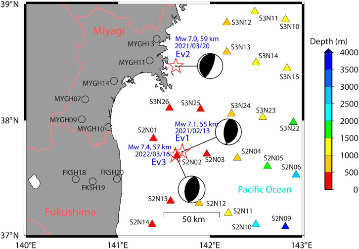
FIGURE 1. Index map. Circles and triangles denote the KiK-net and S-net stations, respectively, used in this study. The S-net stations are color-coded by the depth of water. The stars denote the epicenters of the earthquakes (JMA) used as target events for NLSR analysis. The earthquakes are identified as Ev1, Ev2, and Ev3 according to the order of their occurrences in time. The F-net NIED (Okada et al., 2004) magnitudes (Mw) of the earthquakes were 7.1, 7.0, and 7.4, respectively, while the focal depths were around 55 km. The focal-mechanism plots connected to the epicenters are taken from (Okada et al., 2004) F-net NIED. See Tables 1, 2, and 3 for detail about the earthquakes and sites.

TABLE 1

TABLE 1. Source parameters of earthquakes used in the study.

TABLE 2

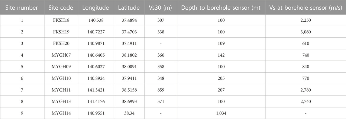
TABLE 2. List of KiK-net site stations used in this study.

TABLE 3

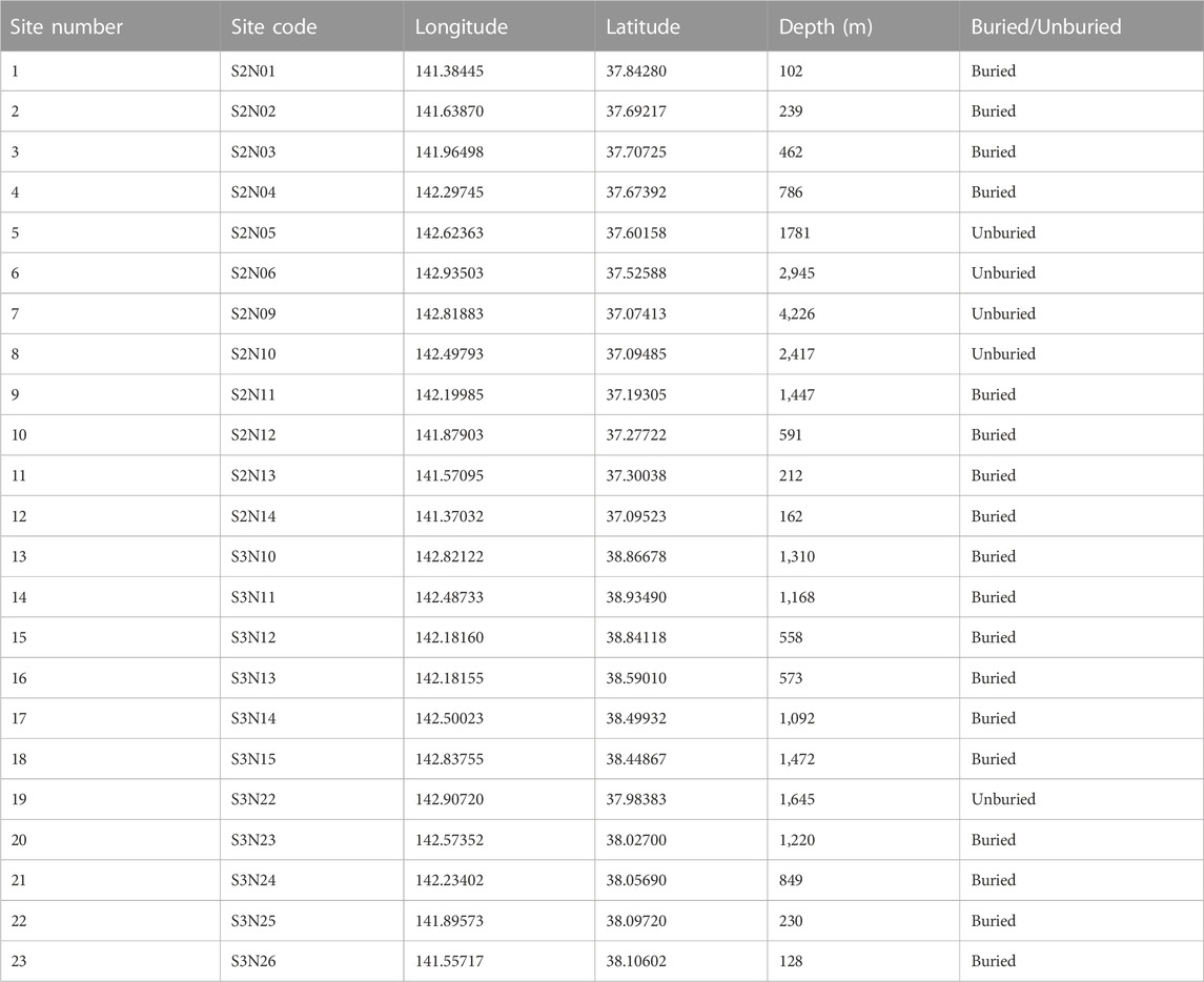
TABLE 3. List of S-net site stations used in this study.

The surface-to-borehole spectral ratio (SBSR) method has been proven to be an effective method to identify the NLSR during strong-motions (e.g., Wen et al., 1994; Satoh et al., 1995; Sato et al., 1996; Sawazaki et al., 2006; Assimaki et al., 2008; Noguchi and Sasatani, 2008; Régnier et al., 2013; Kaklamanos et al., 2015; Noguchi et al., 2016b; Dhakal et al., 2019). This is primarily due to that the borehole sensors have been installed in the stiffer layers, and the variations in source and path factors between the surface and borehole stations are negligible in most cases. This study used the SBSR method to detect NLSR at the nine stations of KiK-net shown in Figure 1. However, as the seafloor observation sites lack the vertical array or reference rock-outcrop sites at near distances, the HVSR method is a suitable one, which has been widely applied in the detection of NLSR during strong-motions (e.g., Noguchi and Sasatani, 2008; Wen et al., 2011; Ren et al., 2017; Ji et al., 2020). The HVSR method utilizes the horizontal and vertical component records observed at the same site. This method was first applied in Wen et al. (2006). We also evaluated the NLSR at the land sites using the HVSR method to compare the results with the SBSR method. For an overview of quantification of nonlinear site response by numerical simulations, we refer to the paper by Régnier et al. (2016) and the references therein.

The SBSRs and HVSRs at the KiK-net stations were calculated using Equations 1 and 2, respectively.

$\mathrm{S}\mathrm{B}\mathrm{S}\mathrm{R}=\sqrt{\frac{{NS}_s^2+{EW}_s^2}{{NS}_b^2+{EW}_b^2}}(1)$

$\mathrm{H}\mathrm{V}\mathrm{S}\mathrm{R}=\sqrt{\frac{{NS}_s^2+{EW}_s^2}{{UD}_s^2}}(2)$

where $NS$, $EW$, and $UD$ denote the acceleration Fourier spectra for the north-south, east-west, and vertical components, respectively. The subscripts, s and b, denote the surface and borehole recordings, respectively.

The S-net seismometers, as mentioned briefly in the previous section, are prone to large induced rotations during strong shakings due to the poor coupling between the sensor houses and seabed sediments. Here, we discuss the example waveforms, their spectrograms based on short-time Fourier transforms (e.g., Rabiner and Schafer, 1978) and Fourier spectra, as depicted in Figure 2. The waveforms plotted in Figure 2 were recorded at the station S2N01 during the 2021 Mw 7.1 earthquake (Ev1 in Table 1). The site was located at the epicentral distance of about 30 km, and the vector PGA of three components was about 560 cm/s². See Figure 1 for the location of the site and epicenter of the earthquake. The upper panels in Figure 2 show the as recorded X-, Y-, and Z-component records from left to right, respectively. X axis coincides with the long axis of the cylindrical pressure vessel, and the Y and Z axes are perpendicular to each other and the X axis. It can be seen in Figure 2 that all the three component records include offsets from about 40 s, the larger offsets being observed on the Y and Z components despite the lower peak accelerations (the absolute values after removing the pre-event mean) compared with the peak value on the X-component record. Before the offsets, distinct ramps can be seen on the Y- and Z-component records (Figures 2B,C). These types of features were reported in several previous studies (Hayashimoto et al., 2019; Nakamura and Hayashimoto, 2019; Takagi et al., 2019; Dhakal et al., 2021). The effects of these offsets are reflected in the spectrograms, Figures 2D–F, as continuous large spectral amplitudes towards the lower end frequencies. The acceleration spectral amplitudes should generally be falling off towards the low-frequency end in the absence of noises. But as also shown in the Fourier spectra plots in Figures 2G–I, they grew up towards the low-frequency end from about 0.3 Hz for the Y and Z components and from about 0.1 Hz for the X component.

FIGURE 2

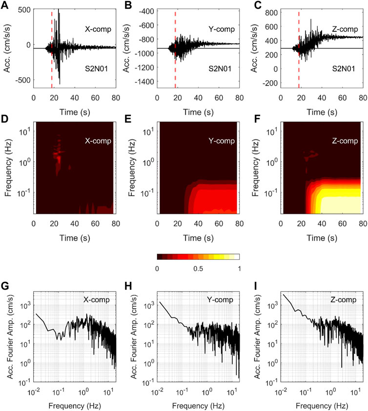
FIGURE 2. Upper panels (A–C) show the as recorded original acceleration time histories at the S2N01 site (buried) for the X, Y, and Z components for the 2021 Mw 7.1 earthquake (Ev1 in Table 1). See Figure 1 for the locations of the site and epicenter of the earthquake. Middle panels (D, E, F) show the time-frequency plots, and bottom panels (G–I) show the Fourier spectra of the waveforms shown in the panels (A, B, C), respectively, after removing the pre-event means of corresponding records. See also the upper three panels of Figure 5, which shows the transformed waveforms into the horizontal and vertical components, respectively.

Another example plot of acceleration time histories recorded at the same site discussed above is given in Figure 3; the records were obtained during the 2021 Mw 7.0 earthquake (Ev2 in Table 1). The site was located at the epicentral distance of about 73 km, and the vector PGA of three components was about 225 cm/s², which is about one-third of the value observed during the previous event (Ev1). The time-history plots in Figures 3A–C do not show visible offsets. The time-frequency plots (Figures 3D–F) show that the S-wave parts contain wide-frequency components, while the later parts are richer at frequencies between about 0.3 and 1 Hz. The Fourier spectra plots in Figures 3G–I show that the rise of spectral amplitudes towards the low-frequency end occurs after about 0.04 Hz, which is lower than those seen in Figures 2G–I for the records of Ev1 discussed above.

FIGURE 3

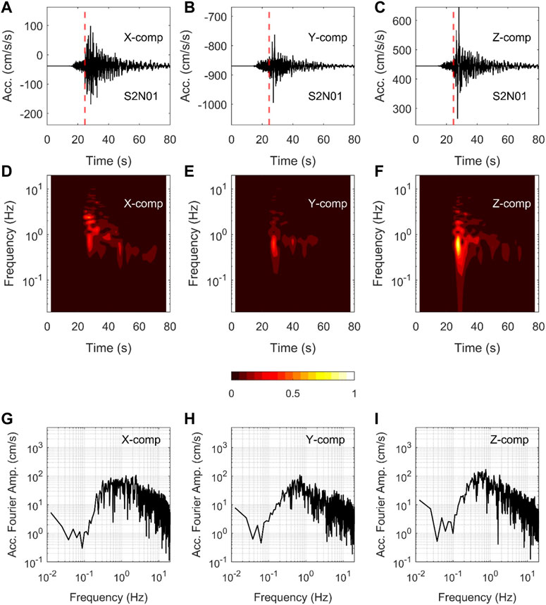
FIGURE 3. Upper panels (A–C) show the as recorded original acceleration time histories at the S2N01 site (buried) for the X, Y, and Z components for the 2021 Mw 7.0 earthquake (Ev2 in Table 1). See Figure 1 for the locations of the site and epicenter of the earthquake. Middle panels (D, E, F) show the time-frequency plots, and bottom panels (G–I) show the Fourier spectra of the waveforms shown in panels (A, B, C), respectively, after removing the pre-event means of corresponding records. See also the lower three panels of Figure 5, which shows the transformed waveforms into the horizontal and vertical components, respectively.

The relationship between the vector PGA of three component records and the induced rotations of the X axis (change in pitch value) and Y (or Z) axis (change in roll value) is given in Figure 4 for the strong-motion records used in the NLSR analysis. Interested readers can find the detailed explanation of pitch and roll angles with illustrations in Takagi et al. (2019). In the present study, the change in pitch and roll were estimated in the following way. The record length was 10 min for each earthquake, beginning from 1 minute before the earthquake origin time. The 1-min time windows at the front and rear ends, respectively, were used to estimate the pitch and roll values at each time step, and the differences in mean pitch and roll values between the two time-windows were calculated. The pitch ($\beta$) and roll ($\gamma$) values at each time step were calculated using Equations 3 and 4, respectively.

$\mathrm{\beta }=-\arcsin \left(\frac{g_x}{g}\right)(3)$

$\mathrm{\gamma }=\arctan \left(\frac{g_y}{g_z}\right)(4)$

where $g$ is the acceleration due to gravity (∼980 cm/s²), and $g_x$, $g_y$, and $g_z$ are the components of $g$ as observed on the $X$, $Y$, and $Z$ component records. The arctan in Equation 4 is a function that returns the four-quadrant inverse tangent of ${\mathrm{g}}_y$ and ${\mathrm{g}}_z$.

FIGURE 4

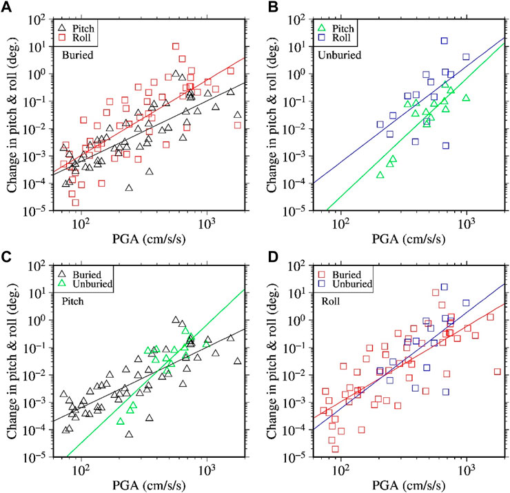
FIGURE 4. Plots of induced rotations of sensors as a function of vector peak accelerations of three component records. The triangles and squares in the plots denote the changes in pitch and roll angles, respectively. Data points in (A) show the changes in pitch and roll angles at the buried stations, while those in (B) show the changes in pitch and roll angles at the unburied stations. Similarly, data points in (C) show the changes in pitch angles, while those in (D) show the changes in the roll angles, at the buried and unburied stations as indicated in the plots. For details on the computation of the pitch and roll angles, see the Data and Method section. The solid lines are the regression lines drawn to aid for the visualization of the mean trend of the corresponding data.

As the S-net accelerometers have not been aligned in the horizontal and vertical directions, different from the common deployments on land, the original records need to be transformed into the horizontal- and vertical-component records to examine the NLSR using the HVSR method. The matrix equation for transformation of the records is given in Equation 5.

$\begin{array}{c}\left[\begin{array}{c}{H}_x\\ H_y\\ V\end{array}\right]\end{array}=\left[\begin{array}{ccc}\cos \beta & \sin \beta \sin \gamma & \sin \beta \cos \gamma \\ 0& \cos \gamma & -\sin \gamma \\ -\sin \beta & \cos \beta \sin \gamma & \cos \beta \cos \gamma \end{array}\right]\left[\begin{array}{c}X\\ Y\\ Z\end{array}\right](5)$

where X, Y, and Z denote the original three component records; $\mathrm{\beta }$ and $\mathrm{\gamma }$ are the pitch and roll angles as defined in Equations 3 and 4, respectively. $H_x$ and $H_y$ denote horizontal component records in the direction of X (cable axis) and perpendicular to it, respectively; $V$ denotes the vertical component record.

For the weak motions, the induced rotations may be considered negligibly small (∼10^–4 degrees or lower). However, the induced rotations during strong shakings can reach to several degrees as shown in Figure 4, and the transformed records may not correctly represent the motions in the horizontal and vertical directions after the ground motions get contaminated by the rotational noises. Example plots of the transformed waveforms after low-cut filtering at 0.1 Hz are shown in Figure 5 for the records drawn in Figures 2 and 3, respectively. In Figure 5, the horizontal X component waveforms for the Ev1 show intermittent acceleration spikes, and the waveforms resemble to some extent to those resulting from the cyclic mobility effects on dilatant soils (e.g., Bonilla et al., 2005). Several records with peak accelerations > about 500 cm/s² exhibited spikes on either horizontal X or Y or both components, while none of the records at the land stations of NIED showed spiky waveforms during the earthquakes. The origin of the spiky waveforms obtained at the S-net stations is not investigated well and is a topic for future study. In the present study, we tried to avoid the effects of offsets and induced-rotational noises in the analysis of NLSR by using the records prior to the offsets, and only 10 s length was used beginning from the S-wave onset. All the records (used from both the land and S-net stations) were low-cut filtered at 0.1 Hz with fourth order Butterworth filter to minimize the low-frequency noises. As the SN ratios are smaller at lower frequencies for the weak motions, we primarily focus on the analysis of NLSR at frequencies between 0.5 and 20 Hz for comparison of the results with previous studies (e.g., Noguchi and Sasatani, 2008; Dhakal et al., 2017).

FIGURE 5

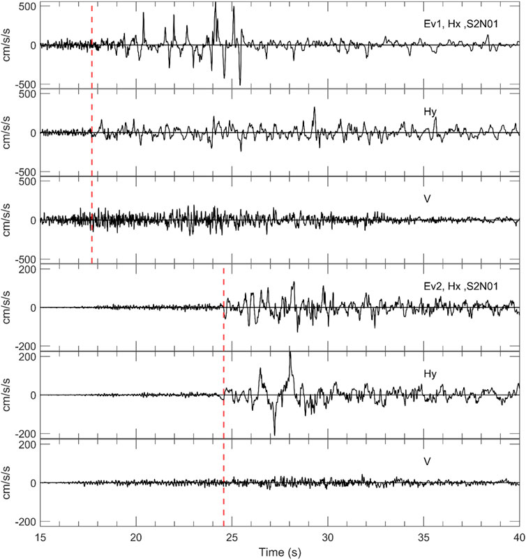
FIGURE 5. The first three traces show the waveforms plotted in Figures 2A–C for the 2021 Mw 7.1 earthquake (Ev1 in Table 1) after transforming them into the horizontal and vertical directions (S2N01 site); the waveforms are shown for the time window between 15 and 40 s after the earthquake origin time for clarity. The two-letter abbreviations Hx and Hy indicate the horizontal components in the direction of and perpendicular to X-axis, respectively. V denotes the vertical component. The lower three traces show the similar plots as described above, but for the waveforms plotted in Figures 3A–C, respectively, for the 2021 Mw 7.0 earthquake (Ev2 in Table 1). The dashed red lines mark the S-wave onsets picked manually. All the waveforms were low-cut filtered at 0.1 Hz.

Although it is beyond the scope of this paper to discuss the detailed features of the peak ground motions from the earthquakes considered in this study, we show the horizontal peak accelerations as a function of the shortest fault-rupture distance and their spatial distribution in Figure 6 for the three events listed in Table 1. See Data Availability Statement for the fault models used to calculate the shortest fault-rupture distances. The values plotted in Figure 6 are the larger ones of peak values of the two horizontal components. The largest peak accelerations of about 1,425, 730, and 1,045 cm/s² were recorded on land for the Ev1 (Mw 7.1), Ev2 (Mw 7.0), and EV3 (Mw 7.4), respectively, at the fault distances of about 75, 64, and 100 km, respectively. The largest peak accelerations at the S-net sites for the three events were about 1,100, 680, and 1730 cm/s², respectively, recorded at the fault distances of about 48, 126, and 48 km, respectively. The peak acceleration data are shown into four groups in each plot in Figure 6. The data from KiK-net sites are grouped into fore-arc (FA) and back-arc (BA) sites while the S-net sites are grouped as buried and unburied sites. It was found that the data generally follow the trends of ground motion prediction curves (Si and Midorikawa, 1999; Si and Midorikawa, 2000) for the three events. However, the BA site records show systematically lower values at longer distances, while the unburied stations, on average, show larger values compared with those at the other site groups. Previous studies (e.g., Kanno et al., 2006; Dhakal et al., 2010; Morikawa and Fujiwara, 2013) showed that the lower Q values in the mantle wedges beneath the volcanic fronts cause stronger attenuation of the high-frequency ground motions passing through them. In contrast, the larger values at the unburied sites may be attributed partly to the lower attenuation of seismic waves in the high-Q Pacific Plate and larger site amplification factors at the unburied sites (Dhakal et al., 2021; Dhakal et al., 2023; Tonegawa et al., 2023).

FIGURE 6

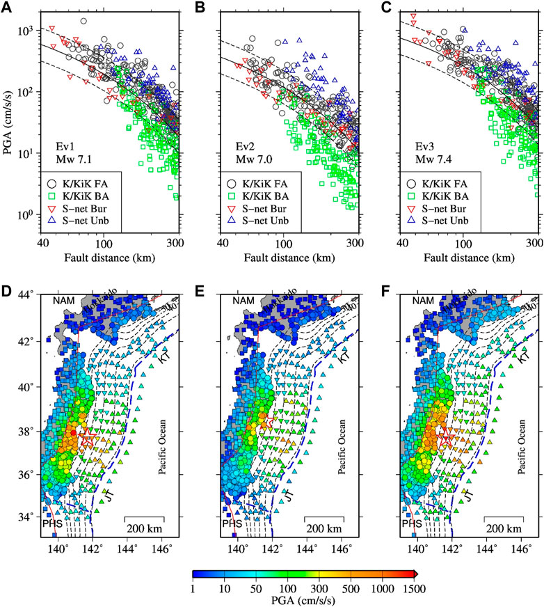
FIGURE 6. Upper panels: PGAs (larger values of two horizontal components) as a function of the shortest fault-rupture distance for three events Ev1, Ev2, and Ev3 (panels (A, B, C)), respectively. The symbols, circle and square, denote the fore-arc and back-arc stations of K-net and KiK-net, written as K/KiK FA and K/KiK BA, respectively, in the legends. The inverted and normal triangles denote the buried and unburied stations of S-net, abbreviated as S-net Bur and S-ne Unb, respectively, in the legends. The solid and dashed lines denote the median prediction curve and range of one standard deviation for soil site condition in the GMPE of Si and Midorikawa (1999) for the corresponding event types (Ev1 and Ev3: intraslab; Ev2: interplate). Lower panel: Spatial distribution of the PGAs for the three events, Ev1, Ev2, and Ev3 (panels (D, E, F)), respectively. Stars denote the epicenters. The dashed blue lines denote the plate boundaries and the red line denotes volcanic front. The dashed grey lines denote the depth contours of the upper surface of the Pacific Plate at interval of 10 km. The 10 km depth contour coincides roughly with the trench axes (JT: Japan Trench and KT: Kurile Trench). The plate-depth data were taken from Hirose (2022). The NAM and PHS are shorthand for the North-American Plate and Philippine Sea Plate, respectively.

Sawazaki and Nakamura (2020) showed that the spectral ratios of coda waves between the $H_y$ and $H_x$ components followed the N-shaped pattern with peaks and troughs at about 7 and 13 Hz, respectively. The characteristic N-shaped pattern were conspicuous at the unburied stations, while the spectral ratios were near unity at many buried stations. We show example plots of the spectral ratios between the $H_y$ and $H_x$ component records at two buried (S2N03 and S2N04) and two unburied (S2N05 and S2N06) stations from the S-wave parts of the records in Figure 7 for the weak and strong motions considered in this study. It can be seen in Figures 7A,B that the mean spectral ratios for the weak motions at the two buried stations are about unity except around 10 Hz. Around the 10 Hz, the mean spectral ratios have small peaks and troughs forming minor-type N-shaped patterns, which are more conspicuous in Figure 7B than in Figure 7A. In contrast, the mean spectral ratios plotted in Figure 7C for the unburied station S2N05 show that the peak value is about four at frequency of around 4 Hz, while the mean spectral ratios plotted in Figure 7D for the unburied station S2N06 do not show a conspicuous peak, but show a steep dip at frequency a little over 10 Hz. These observations are generally similar to those reported in Sawazaki and Nakamura (2020). The strong-motion Hy/Hx spectral ratios at the unburied stations indicate a considerable shift of the N-shaped pattern towards lower frequencies, while the spectral ratios at the buried stations appear to be relatively stable for both weak and strong motions. A further comparison of the Hy/Hx spectral ratios between the weak and strong motions is presented in the discussion section. As a result, we obtained the HVSRs at the S-net stations using the following three equations (Equations 6–8).

$\mathrm{H}\mathrm{V}\mathrm{S}\mathrm{R}\_\mathrm{x}=\frac{H_x}{V}(6)$

$\mathrm{H}\mathrm{V}\mathrm{S}\mathrm{R}\_\mathrm{y}=\frac{H_y}{V}(7)$

$\mathrm{H}\mathrm{V}\mathrm{S}\mathrm{R}\_\mathrm{h}=\sqrt{\frac{H_x^2+H_y^2}{V^2}}(8)$

where $H_x$, $H_y$, and $V$ denote the acceleration Fourier spectra for the horizontal X-component, horizontal Y-component, and vertical-component records, respectively, at the S-net sites. The HVSR and HVSR_h defined in Equations 2, 8 are referred simply as H/V in later figures and can be distinguished easily in the context they appear.

FIGURE 7

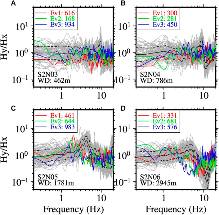
FIGURE 7. Spectral ratios between the horizontal Y- and X-component records at two buried stations [upper panels (A, B)] and two unburied stations [lower panels (C, D)], computed from the S-wave parts of the records. The site code and water depth (WD) are indicated in each panel. The grey lines denote the spectral ratios for individual earthquake records. The black lines denote the mean spectral ratios, while the dashed lines denote the range of one standard deviation. The red, blue, and green lines denote the spectral ratios for the three target earthquakes, denoted by Ev1, Ev2, and Ev3, respectively (see Table 1 for detail about the earthquakes). The numbers nearby the three event codes indicate the larger peak accelerations in units of cm/s² of two horizontal components for the corresponding earthquakes.

Noguchi and Sasatani (2008) proposed the following equation (Equation 9) to express the degree of nonlinearity (DNL) quantitatively.

$\mathrm{D}\mathrm{N}\mathrm{L}={\displaystyle \sum }\left|{\log }_{10}\left\{\frac{R_{strong}}{R_{weak}}\right\}\right|∆f(9)$

where $R_{strong}$ and $R_{weak}$ represent the spectral ratios for strong- and weak-motions, respectively, and $∆f$ is the frequency interval. Noguchi and Sasatani (2008), Noguchi and Sasatani (2011) obtained DNL values from spectral ratios between 0.5 and 20 Hz and suggested threshold DNL values of 2.5 and 4.0 to indicate the NLSR for the SBSR and HVSR methods, respectively. It is to be noted that Equation 9 gives larger weights to higher-frequency components; more than half of the DNL value depends on high-frequency components above 10 Hz (Noguchi and Sasatani, 2008). The suitability of the threshold values to infer NLSR was also confirmed in Dhakal et al. (2017), Dhakal et al. (2019). In the present study also, we computed the DNL values from the spectral ratios between 0.5 and 20 Hz. The frequency distributions of the DNL values for the weak-motion records used in the present study are shown in Figures 8A–E. The mean DNL values were found to be 1.72 and 2.33 for the KiK-net sites with standard deviations of 0.65 and 0.68 for the SBSR and HVSR methods, respectively. Similarly, the mean DNL values for the S-net sites were found to be 2.97 and 2.90 with standard deviations of 0.65 and 0.68 for the HVSR_x and HVSR_y methods, respectively. The mean DNL value for the HVSR_h was found to be 2.60, which may be considered similar to the mean DNL value of 2.33 for the HVSR method at the KiK-net sites considering the range of one standard deviation. The abovementioned DNL values were rounded to two decimal places. Even though the mean DNL values plus the standard deviations in the present analysis using the HVSR, HVSR_x, HVSR_y and HVSR_h methods are lower than the threshold value of 4 considered in the previous studies, it is somewhat difficult to see the reduction in spectral ratios at higher frequencies and the shift of peak frequencies towards the lower ones for smaller DNL values. Thus, the DNL value of 4 may still be considered a reasonable criterion for the preliminary identification of NLSR using the HVSR methods.

FIGURE 8

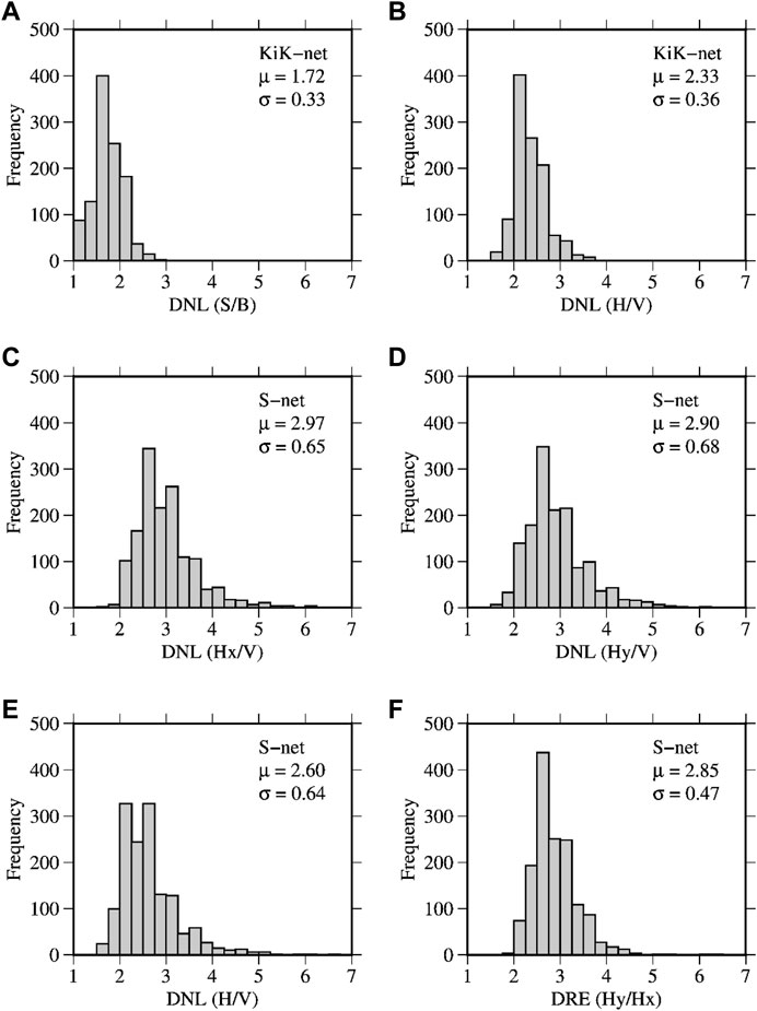
FIGURE 8. Panels (A–E): frequency distributions of the DNL values for the weak-motion records based on the various definitions of the spectral ratios as indicated on the X-axes labels. The panels (A, B) show the plots for the DNL values obtained by using the surface-to-borehole (S/B) and horizontal-to-vertical (H/V) spectral ratio methods, respectively, for the KiK-net sites. The panels (C, D) show the plots for the DNL values obtained by using the Hx/V and Hy/V spectral ratio methods, respectively, for the S-net sites. Panel (E) shows the plot for the DNL values obtained by using the HVSR_h (H/V) spectral ratio method for the S-net sites. Panel (F): frequency distribution of the degree of rotational effect (DRE) described later (see the Discussion section). The mean ($\mu$) and standard deviation ($\sigma$) are indicated in each plot.

Following Derras et al. (2020), we also computed the Arias intensity (AI) (Arias, 1970) and cumulative absolute velocity (CAV) (Reed et al., 1988) to compare with the DNL values using Equations 10 and 11, respectively. Similar to the use of PGAs, the AI and CAV values were also considered as loading levels in the evaluation of NLSR in Derras et al. (2020).

$\mathrm{A}\mathrm{I}=\frac{\pi }{2g}{\displaystyle \underset{0}{\overset{T}{\int }}}{a}^2\left(t\right)dt(10)$

$\mathrm{C}\mathrm{A}\mathrm{V}={\displaystyle \underset{0}{\overset{T}{\int }}}\left|a\left(t\right)\right|dt(11)$

where $a\left(t\right)$ is the acceleration time history, $T$ is the total duration of the time history, and $g$ is an acceleration due to gravity. The time lengths of the recordings at the KiK-net stations have been determined by some threshold accelerations, while the S-net stations record waveforms continuously. To compute the AI and CAV values for the same time lengths at the KiK-net and S-net sites, we fixed the value of $T$ equal to 60 s, starting from S-wave onset.

3 NLSR at the KiK-net sites

Here we show the SBSRs and HVSRs at the KiK-net sites for the three events and discuss the nonlinear features with respect to the corresponding weak-motion spectral ratios. Figure 9 shows the plots of SBSRs at the nine KiK-net sites in panels A to I, respectively. The PGAs (peak vector of two horizontal components), DNL values, and Vs30 values are indicated in each plot. The PGAs at the sites were between about 80 and 1,430 cm/s². For recordings with larger PGAs, the reduction of SBSRs at higher frequency components can be clearly seen with respect to the weak motion SBSRs (e.g., Figure 9A). The plots of the SBSRs show multiple peaks or small undulations at most sites. During strong motions, the peaks of higher frequencies are reduced mostly while the peaks of the lowest peak frequencies are similar to those of the weak-motion recordings at most sites. The shift in peak frequencies can be seen for several recordings as shown in Figures 9A,B,F,H. The threshold DNL value of 2.5 for identifying the NLSR for the SBSR method as discussed in the previous section was exceeded for all recordings except for the Ev2 at MYGH09 site (Figure 9E). The PGA at the MYGH09 site for the Ev2 was approximately 88 cm/s² and was the lowest of all the recordings. The DNL values at the KiK-net sites ranged between 2.4 and 8.2. A larger value of DNL indicates stronger reduction of higher frequency components in the case of typical NLSR. The Vs30 values at the sites ranged between 307 m/s (FKSH18) and 859 m/s (MYGH11). Despite large Vs30 values such as at the MYGH11 (Vs30 = 859 m/s) and MYGH13 (Vs30 = 571 m/s), the features of NLSR were clearly seen at the two sites (see Figures 9G,H). An examination of the PS-logging data indicated soil layers with Vs value of 210 m/s in the top 3 m soil column at the MYGH11 site and 250 m/s in the top 5 m soil column at the MYGH13 site. The presence of these soil layers with lower Vs values might have contributed significantly to the reduction of the higher frequency SBSRs at the two sites.

FIGURE 9

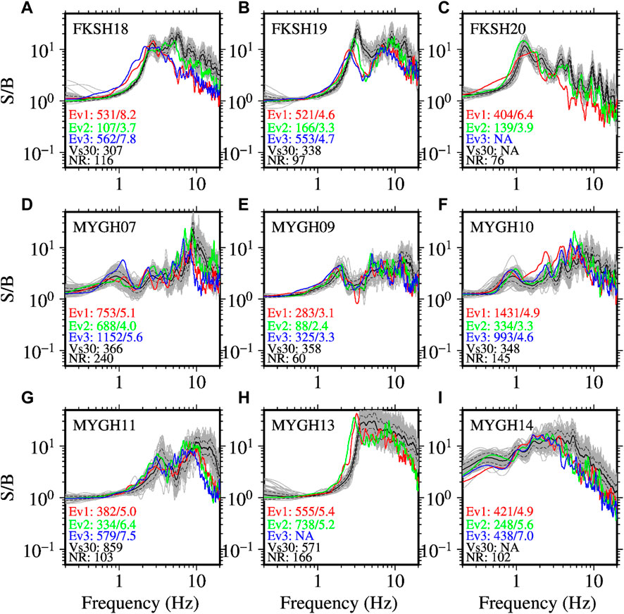
FIGURE 9. Surface-to-borehole (S/B) spectral ratios (SBSR) at the KiK-net sites. The plots (A–I) are arranged in order of site codes as listed in Table 2. The red, green, and blue lines denote the SBSRs for Ev1, Ev2, and Ev3, respectively. The black line denotes the mean SBSRs calculated from weak-motion records (grey lines). The dashed grey lines denote the range of one standard deviation from the mean spectral ratios. The first and second numbers separated by forward slash are the PGA (cm/s²) and DNL values, respectively. Vs30 denotes the average S-wave velocity (m/s) in the upper 30 m soil column, and NR denotes the number of weak-motion records used to compute the mean spectral ratios. The PGAs are the vector peak accelerations of two horizontal components.

The HVSRs at the abovementioned KiK-net sites are shown in Figure 10. The reduction of higher frequency components and shift in peak frequencies can be clearly seen for most of the recordings for the three earthquakes. The change in spectral ratio shapes were generally similar to those of the SBSRs at the corresponding sites. The HVSRs for weak motions show a larger scattering compared to the SBSRs. As a result, the threshold DNL value for identifying the NLSR using the HVSR method is larger compared to the corresponding threshold value for the SBSR method. The obtained DNL values for the HVSR method were between 2.7 and 7.7 in the present analysis.

FIGURE 10

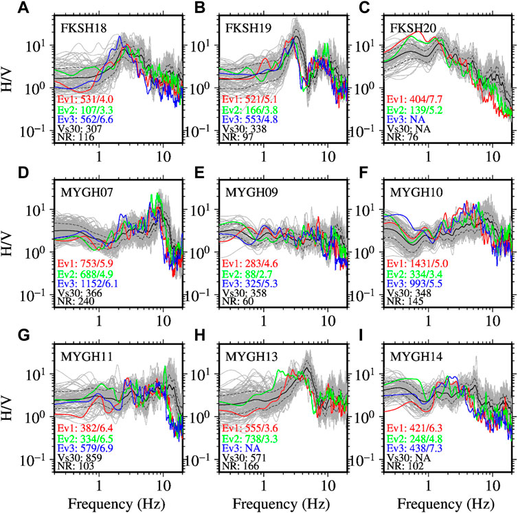
FIGURE 10. Same as Figure 9, but for the horizontal-to-vertical (H/V) spectral ratios (HVSR) at the KiK-net sites. The order of sites in panels (A–I) is identical to that in Figure 9. The HVSRs were computed using Eq. 2. See the caption of Figure 9 for detail.

The relationships between the DNL values and PGAs for the SBSR and HVSR methods are shown in Figures 11A,B, respectively. A general trend of increasing DNL values can be seen with an increase of PGAs. The plot in Figure 11B (HVSR case) shows four points (recordings) with DNL values ≤4 for PGAs >300 cm/s². However, the plot in Figure 11A (SBSR case) shows the DNL values >2.5 for the same recordings, indicating the NLSR. One of the sites with the large difference of the DNL values between the SBSR and HVSR is the MYGH13 site. The DNL values using the HVSR method at the MYGH13 site were 3.6 and 3.3 for the PGAs of 555 and 738 cm/s² for the Ev1 and Ev2, respectively. Nonetheless, the HVSRs clearly showed the shift in peak frequencies. A comparison of the DNL values obtained from the SBSR and HVSR methods is shown in Figure 11C, where it can be seen that the DNL values for the HVSR methods tend to be somewhat larger than those for the SBSR methods for a larger number of recordings (18 versus 7 data points) and are consistent with the previously reported results (e.g., Noguchi and Sasatani, 2011). But it is noted that the largest DNL value among the KiK-net sites is 8.2 in the present analysis and was obtained using the SBSR method. The DNL value of 8.2 was approximately a factor of two of the DNL value obtained using the HVSR method for the corresponding recording (see Figure 9A, 10A for the Ev1). The plots of DNL values for all recordings identified by site and event codes are shown together with the plots for the S-net sites later (see Figure 16).

FIGURE 11

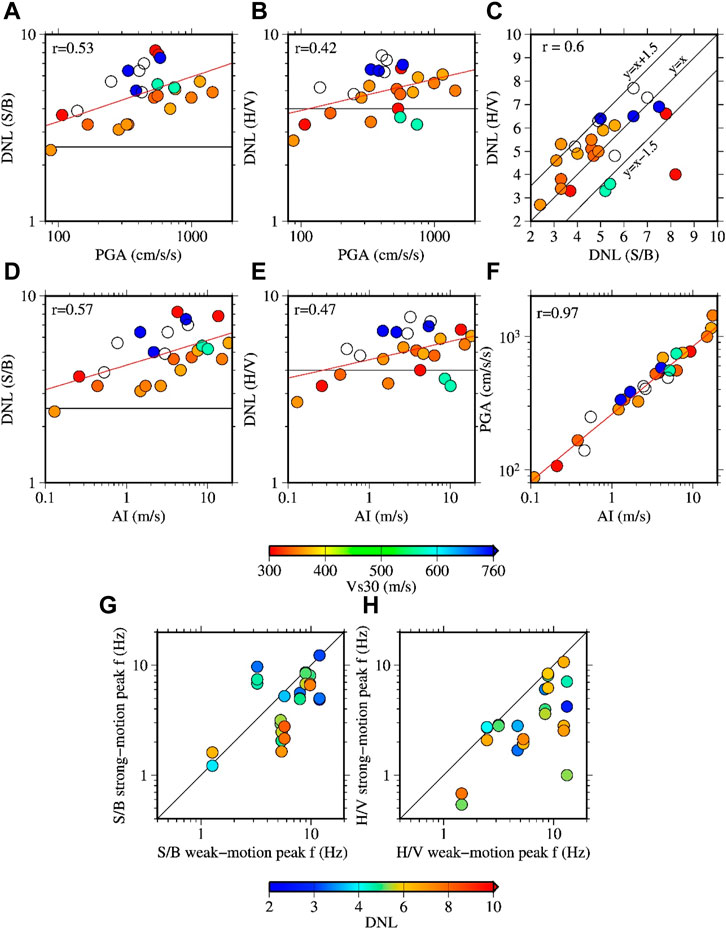
FIGURE 11. Panels (A, B) DNL values based on the SBSR (A) and HVSR (B) methods as a function of the horizontal vector PGAs at the KiK-net sites. The red lines denote the regression lines between the PGAs and DNL values, and the numerals at the upper-left corners indicate the correlation coefficients. Panel (C) comparison of the DNL values between the SBSR and HVSR methods. Panels (D, E) same as panels (A, B) but for the DNL and Arias intensity (AI). Panel (F) relationships between the PGAs and AI values. Panels (G, H) peak frequencies of the spectral ratios during strong and weak motions based on the SBSR (G) and HVSR (H) methods.

The relationships between the DNL and AI values for the SBSR and HVSR methods are shown in Figures 11D,E, respectively. It can be seen that the trends between the DNL and AI values are almost identical to those mentioned above for the DNL and PGAs. This is because the PGAs and AI have a very high correlation, as shown in Figure 11F. The relationships between the DNL and CAV values were also similar to those between the DNL and AI values and are shown in Supplementary Figure S1.

A comparison of the peak frequencies between the weak-motion and strong-motion SBSRs and HVSRs is depicted in Figures 11G, H, respectively. Most of the data points show smaller peak frequencies during the strong motions. A few data points show larger peak frequencies during strong motions compared to the weak-motion peak frequencies. It was found that the difference was simply due to the similar peak ratios at multiple frequencies for the strong motions or the peak frequencies of weak-motion spectral ratios were relatively towards the lower frequencies (e.g., see Figures 9A–C).

4 NLSR at the S-net sites

In this section, the NLSR during the three Mw 7 class earthquakes at the S-net sites are described based on the three types of spectral ratios defined in Equations 6 (HVSR_x), 7 (HVSR_y), and 8 (HVSR_h), respectively. The three types of spectral ratios are referred to simply as Hx/V, Hy/V, and H/V, respectively, for convenience. The number of S-net sites used in the analysis is 23. Therefore, to save space and reduce monotony, example plots of the HVSRs are shown here for only 8 sites, and the plots of the HVSRs at all the remaining sites are provided in the Supplementary Figure S2, S3, S4, S5. The plots of the HVSRs at the S2N01, S2N02, S2N03, and S2N04 are shown in Figure 12. Similarly, the plots of the HVSRs at the S2N05, S2N06, S2N09, and S2N10 are shown in Figure 13. For each site, the HVSRs based on the three equations (Equations 6, 7, and 8) are shown in three different plots. For example, the plots of the Hx/V, Hy/V, and H/V at the S2N01 site are shown in Figures 12A–C, respectively. The plots follow similarly for the other sites. The PGAs of the horizontal X-component records for the three target earthquakes were between about 50 and 1740 cm/s², respectively.

FIGURE 12

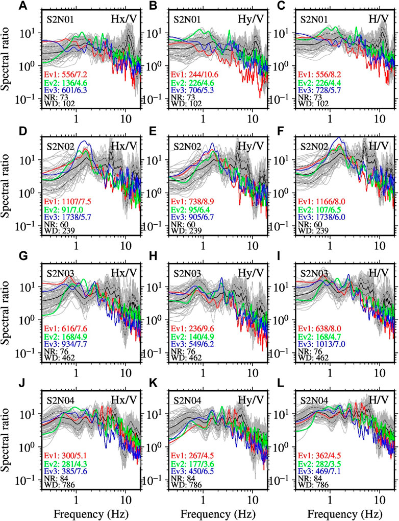
FIGURE 12. Example plots of the HVSRs at the S-net sites. The plots (A, B, C) in the top panels show the spectral ratios between the horizontal X and vertical component records (Hx/V; Equation 6), horizontal Y and vertical component records (Hy/V; Equation 7), and vector of two horizontal components and vertical component records (H/V; Equation 8), respectively, at the S2N01 site. The other plots follow similarly for the records at the S2N02 (D, E, F), S2N03 (G, H, I), and S2N04 (J, K, L) sites, respectively. WD denotes the depth (m) to the seafloor. The events and related values are identified by the same color schemes as explained in the caption of Figure 9.

FIGURE 13

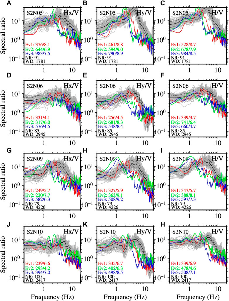
FIGURE 13. Same as Figure 12, but for the sites S2N05 (A, B, C), S2N06 (D, E, F), S2N07 (G, H, I), and S2N10 (J, K, L), respectively. See the caption of Figure 12 for detail. See Supplementary Figures S2–S5 for the plots of the HVSRs at the other sites.

In Figures 12A–C (plots for the S2N01 site), it can be seen that the weak-motion spectral ratios have a dominant peak at frequency of a little over 10 Hz. In contrast, the values of the spectral ratios become noticeably smaller for the strong motions at the dominant frequency of weak-motion spectral ratios. Reduction of amplitude of the spectral ratios at higher frequencies compared with the weak-motions was clearly seen for most of the recordings at all the sites. Also, a shift of the peak frequency of the spectral ratios was clearly observed for many recordings. This last feature can be seen well in Figure 13. The DNL values for the case of Hx/V ranged between 3.3 and 9.6, while those for the case of Hy/V ranged between 3 and 10.6. The DNL values for the case of H/V were between 2.8 and 9.8.

The plots of DNL values as a function of PGAs for the three definitions of HVSRs are shown in Figures 14A–F for the buried and unburied sites separately. A general trend of increasing DNL values with PGAs can be seen in all the plots for both groups of data. Note that the peak values reported in the HVSR plots and discussed here are from the S-wave window only. A comparison of the DNL values based on the Hx/V and Hy/V spectral ratios is shown in Figures 14G,H, respectively. It was found that the DNL values for the case of Hy/V were somewhat larger than those for the Hx/V case for the recordings that accompanied the larger rotations of the sensors. These features were more obvious for the unburied site conditions. The relationships of the DNL values with AI and CAV are given in Supplementary Figure S6, S7, where results similar to that of the DNL and PGA discussed above can be seen due to the high correlation between the PGAs, AI and CAV values.

FIGURE 14

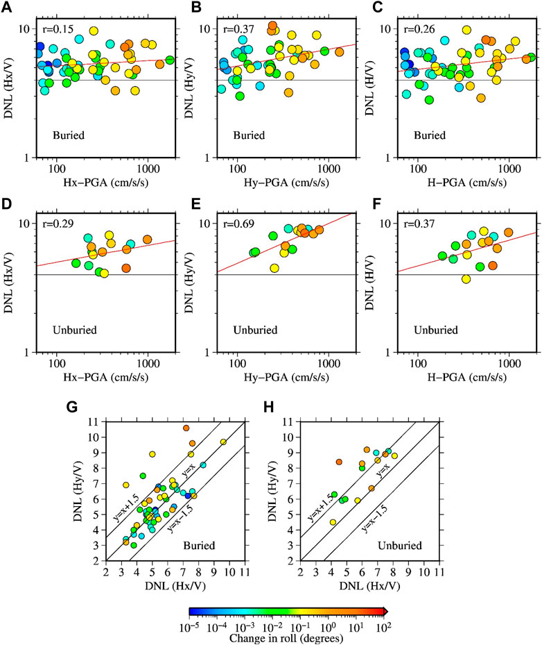
FIGURE 14. DNL values as a function of the PGAs at the S-net sites (A–F). The top (A, B, C) and middle (D, E, F) panels show the plots for the buried and unburied sites, respectivly, for the three different definitions of spectral ratios given in Equations 6, 7, and , 8, respectively. The x-axes labels, Hx-PGA, Hy-PGA, and H-PGA mean the peak acceleration of the horizontal X, horizontal Y, and vector of the two horizontal component records, respectively. The red lines denote the regression lines between the corresponding PGAs and DNL values, and the numerals at the upper-left corners indicate the correlation coefficients. The bottom panels show the relationships between the DNL values based on the Hx/V and Hy/V spectral ratios at the buried (G) and unburied (H) sites, respectively.

A comparison of the peak frequencies between the weak-motion and strong-motion spectral ratios is depicted in Figure 15 for the buried and unburied sites separately. The figure shows that the peak frequencies of the strong-motion spectral ratios are mostly smaller than those of the weak-motion spectral ratios at frequencies over about 3 Hz. The unburied sites have weak-motion peak frequencies of about 2 Hz or higher and the above feature can be seen clearly. At the buried sites, the peak frequencies of the strong-motion spectral ratios are not always smaller than those of the weak-motion spectral ratios. We found that this is mainly due to the comparable peak values of the spectral ratios at two different frequencies.

FIGURE 15

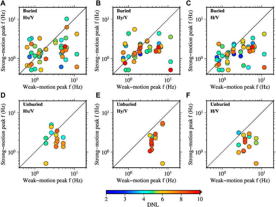
FIGURE 15. Relationships between the peak frequencies of the weak-motion and strong-motion spectral ratios for the recordings obtained at the S-net sites. The upper (A, B, C) and lower (D, E, F) panels show the plots for the buried and unburied sites, respectivly, for the different definitions of spectral ratios (see the caption of Figure 12 for detail).

5 Discussions

In this section we first discuss the relationships of the DNL values and shift in peak frequencies between the KiK-net and S-net sites. A combined plot of the DNL values for the KiK-net and S-net sites as a function of the PGAs is shown in Figure 16A. Similarly, a combined plot for the KiK-net and S-net sites of the relationship between the peak frequencies of the spectral ratios for the strong- and weak-motions is shown in Figure 16B. It can be seen that the values between the two data sets (KiK-net and S-net) distribute generally similarly except at lower PGAs and lower weak-motion peak frequencies. It is notable that the DNL values are larger than the threshold value of 4 for several recordings at the S-net sites at PGAs lower than about 200 cm/s². The DNL values based on the SBSR and HVSR methods at the KiK-net sites for all event-site pairs are shown in Figures 16C,D, respectively, while the similar plots for the Hx/V and Hy/V methods at the S-net sites are summarized in Figures 16E,F, respectively. In these plots, it can be clearly noticed the changes in the DNL values with PGAs at the same site.

FIGURE 16

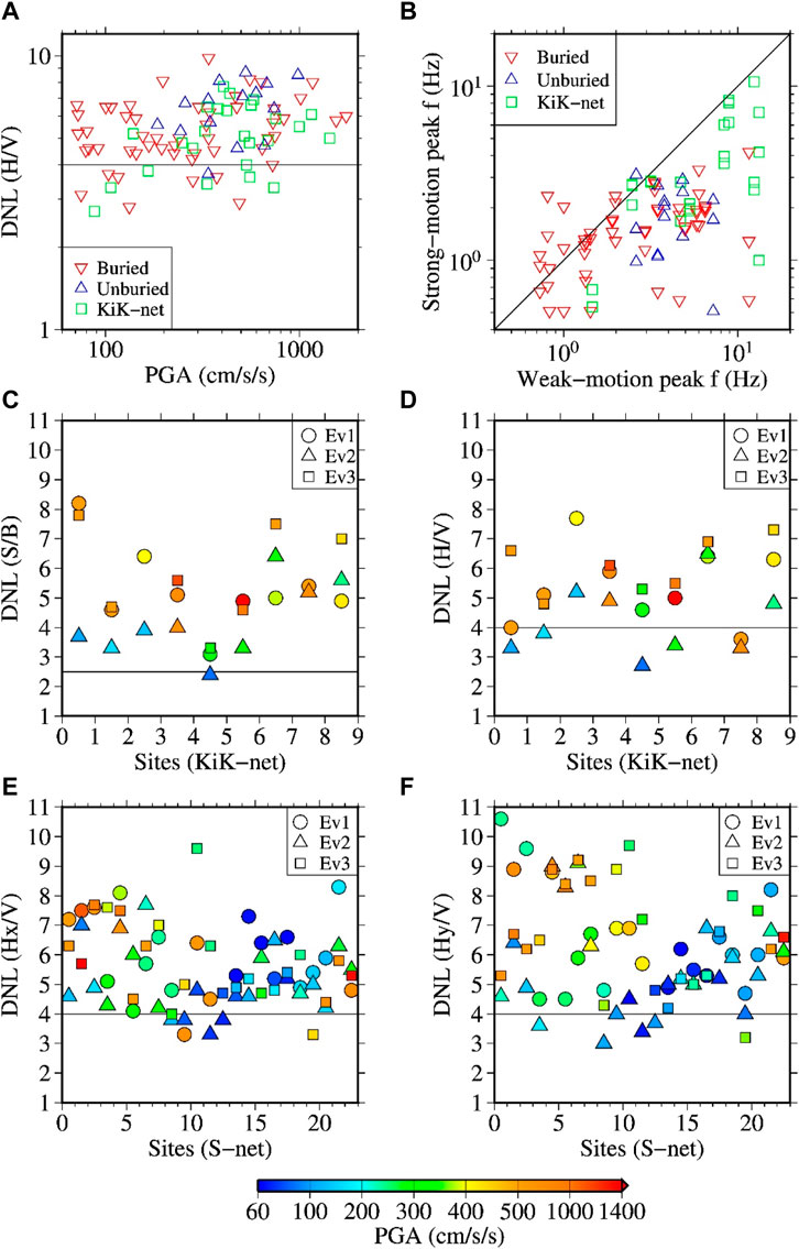
FIGURE 16. Panel (A) comparison of the DNL values as a function of the horizontal vector PGAs between the KiK-net and S-net (Buried and Unburied) sites. Panel (B) comparison of the peak frequencies of the HVSRs during the weak and strong motions. The HVSRs for the KiK-net and S-net sites were computed identically using Equations 2 and 8, respectively. Panel (C, D): DNL values at the KiK-net sites using the SBSR and HVSR methods, respectively. Panel (E, F): DNL values at the S-net sites using the Hx/V and Hy/V methods, respectively. The tick labels of the X-axes in the panels (C–F) indicate the site identification numbers as listed in Tables 2 and 3 for the KiK-net and S-net sites, respectively. The DNL value for a site is plotted 0.5 unit left of its site identification number in the panels C–F.

Even though the measured S-wave velocities are not available for the local soil profiles at the S-net sites, recent studies based on H/V analysis of ambient noise recordings (e.g., Farazi et al., 2023) and seismic interferometric techniques (e.g., Spica et al., 2020; Yamaya et al., 2021; Viens et al., 2023), have revealed the existence of relatively low Vs values in the area around the S-net stations. For example, Farazi et al. (2023) estimated Vs value of about 30 m/s in the top 1.3–1.8 m seabed sediments, and 200–2000 m/s in the next several hundred meters beneath the seafloor, the velocity being increased with depth. Similarly, Viens et al. (2023) suggested a Vs value of about 200 m/s in the shallow layers at some sections of their distributed acoustic sensing profiles. Using the relatively lower amplitude motions than those used in the present study, Viens et al. (2022) reported some signatures of NLSR in the Tohoku offshore region.

A variation of S-wave velocity in the shallow part of the overriding plate beneath the S-net stations was investigated in Tonegawa et al. (2023). The study found a significant reduction of S-wave velocity associated with the large ground motions during Mw six to seven class earthquakes, including the three earthquakes analyzed in the present study. The reduction in S-wave velocity was significant even at longer distances near the Trench axis due to effective trapping of the seismic energy in the upper part of the Pacific Plate. These findings in Tonegawa et al. (2023) support the results shown in the current study, such as the shift in predominant frequencies during strong motions due to reductions of velocity in the shallow sediment layers. The existence of lower Vs values in the shallow layers can produce stronger NLSR during larger input motions. Dhakal et al. (2017) and Kubo et al. (2019), using the same technique as used in the present study, reported that a few offshore sites in the Sagami Trough and Nankai Trough area, respectively, might have experienced NLSR for recordings with PGAs smaller than 100 cm/s². All the above discussions and results may suggest that the S-net sites are prone to experience a large degree of NLSR during major earthquakes in the region.

Finally, we discuss that the so-called NLSR presented above for the S-net sites may have been contaminated by the induced rotation of the sensors. We obtained a DNL-like parameter between the weak-motion and strong-motion Hy/Hx spectral ratios for the same set of data used in the computation of the DNL values. The new parameter is called ‘degree of rotational effect’, abbreviated as DRE for simplicity. The DRE value was also obtained from the same frequency limits, 0.5–20 Hz, as used in the computation of the DNL values. The frequency distribution of the DRE values for the weak motions is shown in Figure 8F. The mean DRE value was found to be 2.85 with standard deviation of 0.47. The DRE values for the target strong-motion records were approximately between 2 and 7. Their relationships with PGAs and DNL values are explained in the next paragraph. The Hy/Hx spectral ratios during the three Mw 7 class earthquakes for the first 12 sites, as listed in Table 3, are compared with the weak-motion Hy/Hx spectral ratios in Figure 17. A similar comparison is shown in Supplementary Figure S8 of the Supplementary File for the remaining 11 sites. The buried stations did not show the typical N-shaped spectral ratios during both weak and strong motions, while three stations out of five unburied stations considered in this study showed the shift in the N-shaped pattern, giving larger DRE values. The three unburied stations are S2N05 (Figure 17E), S2N06 (Figure 17F), and S3N22 (Supplementary Figure S8G). The DRE values at the other two unburied stations were also relatively larger compared with the similar PGA records at buried stations. At a few buried stations such as S2N04 and S2N11 (Figures 17D,I), minor-type N-shaped pattern can be seen around 10 Hz, as mentioned in the Data and Method section. The Hy/Hx spectral ratios for the strong motions were either smooth around the minor-type N-shaped pattern, or they shifted moderately towards lower frequencies. As the computation method for DRE gives larger weights to higher frequencies, relatively larger DRE values were obtained at theses buried sites with the minor-type N-shaped pattern around 10 Hz in comparison to those which did not have the N-shaped spectral ratios.

FIGURE 17

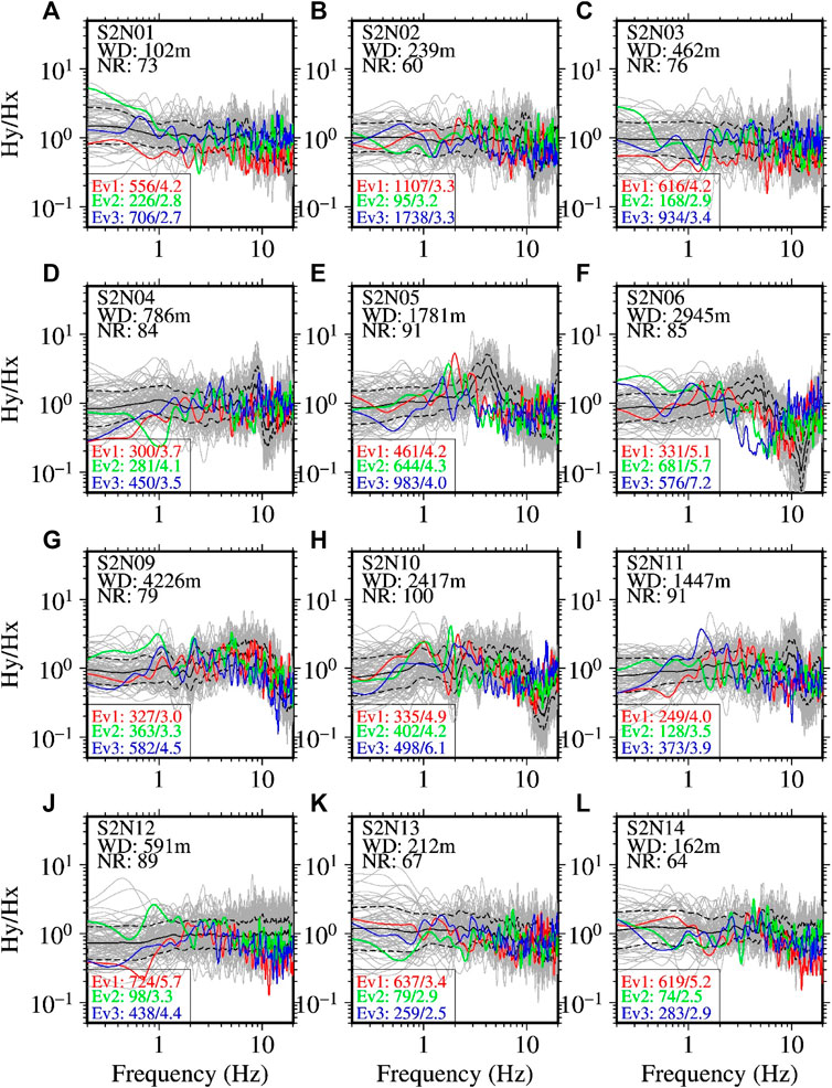
FIGURE 17. Spectral ratios between the horizontal Y- and X-component records at the S-net sites [panels (A–L)]. The site codes are indicated in each panel. The two letter codes, WD and NR written beneath the site codes, indicate the water depth and number of weak-motion records at each site. The grey lines denote the spectral ratios for individual earthquake records. The black lines denote the mean spectral ratios, while the dashed lines denote the range of one standard deviation. The red, blue, and green lines denote the spectral ratios for the three target earthquakes, denoted by Ev1, Ev2, and Ev3, respectively (see Table 1 for detail about the earthquakes). The numbers nearby the event codes separated by forward slash (e.g., Ev1: 724/5.7 in panel J) indicate the larger peak acceleration in units of cm/s² of two horizontal components and the DRE value for the corresponding earthquake. See Supplementary Figure S8 for similar plots at the other sites.

Plots of the DRE values against the PGAs and DNL values are shown in Figure 18 (A-F) and (G-L), respectively. A moderate positive correlation was found between the DRE and PGA values for the buried sites. The range of PGAs was smaller for the unburied sites compared to that for the buried sites, and hence the trend of DRE values with PGAs was not clearly seen. The DNL values obtained for both Hx/V and Hy/V methods correlated poorly with the DRE values and were inconsistent with the DRE values for the data set considered in this study. The station-wise plots of the DRE values annotated with corresponding PGAs and DNL values are shown in Figures 19A–D, respectively. The DRE values at many sites were larger with higher PGAs at the sites. However, the DRE values at several sites did not show a consistent trend with DNL values based on the Hx/V method, while they were generally larger with larger DNL values based on the Hy/V method. These last results may imply that the NLSR at a site appears to be larger using the Hy/V method without considering the induced rotational effect of the sensors on the recorded Y-component motions.

FIGURE 18

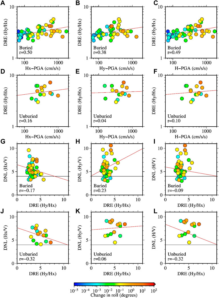
FIGURE 18. Panels (A–F) show the relationships between the DRE and PGA values at the buried and unburied sites of S-net as indicated in the plots. The x-axes labels, Hx-PGA, Hy-PGA, and H-PGA mean the peak acceleration of the horizontal X, horizontal Y, and vector of the two horizontal component records, respectively. The red lines denote the regression lines between the corresponding values, and the numerals at the lower-left corners indicate the correlation coefficients. Panels (G–L) show the relationships between the DNL and DRE values at the buried and unburied sites as indicated in the plots.

FIGURE 19

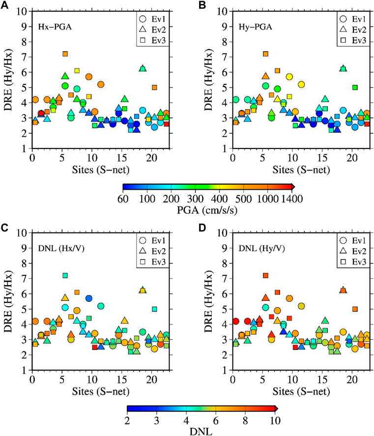
FIGURE 19. Panels (A) and (B) DRE values with annotations by Hx-PGA and Hy-PGA, respectively, at the S-net sites. The tick labels of the X-axes indicate the site identification numbers as listed in Table 3 for the S-net sites. Panels (C) and (D) similar to the panels A and B, but with the annotations by DNL values obtained for the Hx/V and Hy/V cases, respectively.

6 Conclusion

We used the horizontal-to-vertical spectral ratio (HVSR) technique to identify the nonlinear site response (NLSR) at the S-net seafloor observation sites during three Mw 7 class earthquakes. During these earthquakes, large peak ground accelerations were recorded at both onshore and offshore stations. Ramps and significant offsets were seen on some of the acceleration records of S-net with intermittent spikes on accelerations exceeding about 500 cm/s².

We used the initial 10 s of the S-wave portions of the records to compute the Fourier spectra for the analysis of HVSRs. This 10 s time window avoided the offsets on the acceleration records. The effect of ramp was minimized by applying low-cut filter at 0.1 Hz. Considering the resonance effect of the S-net sensor houses on the two horizontal components, the HVSRs were computed for each of the horizontal components separately and also for the two horizontal components jointly. Because the qualities of the S-net strong-motion records with high peak accelerations are in doubt due to the issues related with the poor coupling between the sensor houses and the sediments, we first evaluated the NLSR at the KiK-net sites on land, where high quality records were obtained at surface and borehole.

We used the surface-to-borehole spectral ratio (SBSR) and HVSR method to examine the features of NLSR at nine KiK-net sites common to the three events. In these methods, reference spectral ratios are first obtained using weak-motion records for which the site response is mostly linear. Then, the spectral ratios obtained for the records with larger PGAs during the target earthquakes were compared with the weak-motion spectral ratios. We found that the two most common features of the NLSR, the reduction of higher frequency spectral ratios and shift of peak frequencies, were present for most of the recordings at the KiK-net sites analyzed in this study.

By performing the similar analysis of HVSRs at the S-net sites, we found that the S-net sites also experienced various degrees of NLSR during the three earthquakes. The degree of nonlinearity (DNL) values obtained in this study were similar between the KiK-net and S-net sites within the range of comparable peak accelerations with larger data points (between about 300 and 800 cm/s²). The DNL values increased with the increase of recorded peak accelerations at the both KiK-net and S-net sites on average. The relationship between the weak-motion and strong-motion peak frequencies for the S-net sites were also generally similar to those seen for the KiK-net sites. We found that the reduction of spectral ratios occurred mostly at frequencies higher than about 2 Hz. The shift in peak frequencies were also common for sites with weak-motion peak frequencies higher than 1 Hz. The amplification effect at frequencies lower than about 1 Hz was not so evident associated with the shift in peak frequencies except at few sites.

The DNL values based on the Hy/V spectral ratios were somewhat larger than those based on the Hx/V spectral ratios, and this difference was more evident at the unburied sites. The shift in peak frequencies were also more obvious in the Hy/V spectral ratios. These component-wise differences were most probably related with the different degrees of rotations of the X and Y axes of the sensors even in the S-wave windows used in this study. An analysis of the Hy/Hx spectral ratios during the strong and weak motions indicated a distinct effect of induced rotations at the unburied stations. To some extent, the radiation pattern and directivity effects may have also caused the discrepancies between the two horizontal components, and hence between the Hx/V and Hy/V spectral ratios. Nonetheless, the general similarities of the results between the KiK-net and S-net sites for the same set of earthquakes suggests that the S-net sites are prone to undergo NLSR widely during major offshore earthquakes due to the presence of relatively softer sediments in the top layers. Analysis of the data from broad magnitude ranges and various source-to-site distances is expected to elucidate further the degrees of NLSR at the S-net sites. Based on the present analysis of Mw 7 class earthquake records at relatively short distances, it is concluded that the analysis of strong ground motions at the S-net sites requires consideration of the NLSR, but considersation of the effects of induced rotations of the sensors is necessary to understand the NLSR at the S-net sites better.

Data availability statement

The K-NET and KiK-net strong-motion records and the Vs30 values at the KiK-net sites used in this study were obtained from the website http://www.kyoshin.bosai.go.jp/. The S-net records were obtained from the website https://hinetwww11.bosai.go.jp/auth/download/cont/?LANG=en. The hypocenter information of the events were taken from https://www.data.jma.go.jp/svd/eqev/data/bulletin/hypo_e.html. The moment magnitude for the events were taken from http://www.fnet.bosai.go.jp/event/joho.php?LANG=en. The fault models used to calculate the shortest fault-rupture distance to the sites were obtained from the following websites (in Japanese). Ev1:https://www.kyoshin.bosai.go.jp/kyoshin/topics/FukushimakenOki_20210213/inversion/inv_index.html Ev2:https://www.kyoshin.bosai.go.jp/kyoshin/topics/MiyagikenOki_20210320/inversion/inv_index.html Ev3:https://www.hinet.bosai.go.jp/topics/off-fukushima220316/?LANG=ja&m=source All the above links were last accessed on 2023/03/01.

Author contributions

YD performed analysis of data and drafted the manuscript. TK guided the first author through the data processing and interpretation. All authors contributed to the article and approved the submitted version.

Funding

This study was supported by “Advanced Earthquake and Tsunami Forecasting Technologies Project” of NIED and JSPS KAKENHI Grant Number JP20K05055.

Acknowledgments

We would like to thank the Japan Meteorological Agency for providing us with hypocenter information for the earthquakes used in this study. We would also like to thank Wessel and Smith (1998) for providing us with Generic Mapping Tools, which were used to make some figures in the manuscript. We express our gratitude to Hisahiko Kubo for providing us with the fault plane data, which were used to calculate the shortest fault distances at the observation sites. We are very thankful to the reviewers for providing us with helpful and constructive comments.

Conflict of interest

The authors declare that the research was conducted in the absence of any commercial or financial relationships that could be construed as a potential conflict of interest.

Publisher’s note

All claims expressed in this article are solely those of the authors and do not necessarily represent those of their affiliated organizations, or those of the publisher, the editors and the reviewers. Any product that may be evaluated in this article, or claim that may be made by its manufacturer, is not guaranteed or endorsed by the publisher.

Supplementary material

The Supplementary Material for this article can be found online at: https://www.frontiersin.org/articles/10.3389/feart.2023.1180289/full#supplementary-material

References

Aoi, S., Asano, Y., Kunugi, T., Kimura, T., Uehira, K., Takahashi, N., et al. (2020). Mowlas: NIED observation network for earthquake, tsunami and volcano. Earth Planets Space 72, 126. doi:10.1186/s40623-020-01250-x

CrossRef Full Text | Google Scholar

Arias, A. (1970). “A measure of earthquake intensity,” in Seismic design for nuclear power plants. Editor R. Hansen (Cambridge, Massachusetts: MIT Press), 438–483.

Google Scholar

Assimaki, D., Li, W., Steidl, J. H., and Tsuda, K. (2008). Site amplification and attenuation via downhole array seismogram inversion: A comparative study of the 2003 miyagi-oki aftershock sequence. Bull. Seismol. Soc. Am. 98, 301–330. doi:10.1785/0120070030

CrossRef Full Text | Google Scholar

Barnes, C. R., Best, M. M. R., Johnson, F. R., and Pirenne, B. (2015). “NEPTUNE Canada: Installation and initial operation of the world’s first regional cabled ocean observatory,” in Seafloor observatories (Berlin, Heidelberg: Springer Praxis Books). doi:10.1007/978-3-642-11374-1_16

CrossRef Full Text | Google Scholar

Beresnev, I. A., and Wen, K. L. (1996). Nonlinear soil response - a reality? Bull. Seismol. Soc. Am. 86, 1964–1978. doi:10.1785/BSSA0860061964

CrossRef Full Text | Google Scholar

Bonilla, L. F., Archuleta, R. J., and Lavallée, D. (2005). Hysteretic and dilatant behavior of cohesionless soils and their effects on nonlinear site response: Field data observations and modeling. Bull. Seismol. Soc. Am. 95, 2373–2395. doi:10.1785/0120040128

CrossRef Full Text | Google Scholar

Derras, B., Bard, P. Y., Régnier, J., and Cadet, H. (2020). Non-linear modulation of site response: Sensitivity to various surface ground-motion intensity measures and site-condition proxies using a neural network approach. Eng. Geol. 269, 105500. doi:10.1016/j.enggeo.2020.105500

CrossRef Full Text | Google Scholar

Dhakal, Y. P., and Kunugi, T. (2021). An evaluation of strong-motion parameters at the S-net ocean-bottom seismograph sites near the Kanto basin for earthquake early warning. Front. Earth Sci. 9, 699439. doi:10.3389/feart.2021.699439

CrossRef Full Text | Google Scholar

Dhakal, Y. P., Takai, N., and Sasatani, T. (2010). Empirical analysis of path effects on prediction equations of pseudo-velocity response spectra in northern Japan. Earthq. Eng. Struct. Dyn. 39, 443–461. doi:10.1002/eqe.952

CrossRef Full Text | Google Scholar

Dhakal, Y. P., Shin, A., Kunugi, T., Suzuki, W., and Kimura, T. (2017). Assessment of nonlinear site response at Ocean bottom seismograph sites based on S-wave horizontal-to-vertical spectral ratios: A study at the Sagami bay area K-net sites in Japan. Earth, Planets Space 69, 29. doi:10.1186/s40623-017-0615-5

CrossRef Full Text | Google Scholar

Dhakal, Y. P., Kunugi, T., Kimura, T., Suzuki, W., and Aoi, S. (2019). Peak ground motions and characteristics of nonlinear site response during the 2018 Mw 6.6 Hokkaido eastern Iburi earthquake. Earth, Planets Space 71, 56. doi:10.1186/s40623-019-1038-2

CrossRef Full Text | Google Scholar

Dhakal, Y. P., Kunugi, T., Suzuki, W., Kimura, T., Morikawa, N., and Aoi, S. (2021). Strong motions on land and Ocean bottom: Comparison of horizontal PGA, PGV, and 5% damped acceleration response spectra in northeastnortheast Japan and the Japan Trench area. Bull. Seism. Soc. Am. 111, 3237–3260. doi:10.1785/0120200368

CrossRef Full Text | Google Scholar

Dhakal, Y. P., Kunugi, T., Yamanaka, H., Wakai, A., Aoi, S., and Nishizawa, A. (2023). Estimation of source, path, and site factors of S waves recorded at the S-net sites in the Japan Trench area using the spectral inversion technique. Earth, Planets Space 75, 1. doi:10.1186/s40623-022-01756-6

CrossRef Full Text | Google Scholar

Farazi, A. H., Ito, Y., Garcia, E. S. M., Lontsi, A. M., Sánchez-Sesma, F. J., Jaramillo, A., et al. (2023). Shear wave velocity structure at the Fukushima forearc region based on H/V analysis of ambient noise recordings by ocean bottom seismometers. Geophys. J. Int. 233 (3), 1801–1820. doi:10.1093/gji/ggad028

CrossRef Full Text | Google Scholar

Hardin, B. O., and Drnevich, V. P. (1978). Shear modulus and damping in soils: Design equations and curves. J. soil Mech. Found. Div. 98 (SM7), 667–692. doi:10.1061/jsfeaq.0001760

CrossRef Full Text | Google Scholar

Hayashimoto, N., Nakamura, T., and Hoshiba, M. (2014). “The characteristics of unusual OBS data exposed to strong shaking and the influence of applying these data to EEW processing: Examples of off-kushiro OBS, JAMSTEC,” in AGU fall meeting, S33C–S4543.

Google Scholar

Hayashimoto, N., Nakamura, T., and Hoshiba, M. (2019). A technique for estimating the UD-component displacement magnitude for earthquake early warnings that can be applied to various seismic networks including ocean bottom seismographs. Q. J. Seismol. 83, 1–10. (in Japanese with English abstract).

Google Scholar

Hirose, F. (2022). Plate configuration. Available from: https://www.mri-jma.go.jp/Dep/sei/fhirose/plate/en.index.html (Accessed May 10, 2022).

Google Scholar

Hsiao, N. C., Lin, T. W., Hsu, S. K., Kuo, K. W., Shin, T. C., and Leu, P. L. (2014). Improvement of earthquake locations with the marine cable hosted observatory (MACHO) offshore NE taiwan. Mar. Geophys Res. 35, 327–336. doi:10.1007/s11001-013-9207-3

CrossRef Full Text | Google Scholar

Hu, J., Tan, J., and Zhao, J. X. (2020). New GMPEs for the Sagami Bay Region in Japan for moderate magnitude events with emphasis on differences on site amplifications at the seafloor and land seismic stations of K-NET. Bull. Seism. Soc. Am. 110, 2577–2597. doi:10.1785/0120190305

CrossRef Full Text | Google Scholar

Idriss, I. M., and Seed, H. B. (1968). Seismic response of horizontal soil layers. J. soil Mech. Found. Div. 94 (SM4), 1003–1031. doi:10.1061/jsfeaq.0001163

CrossRef Full Text | Google Scholar

Ji, K., Wen, R., Ren, Y., and Dhakal, Y. P. (2020). Nonlinear seismic site response classification using K-means clustering algorithm: Case study of the September 6, 2018 Mw6.6 Hokkaido Iburi-Tobu earthquake, Japan. Soil Dyn. Earthq. Eng. 128, 105907. doi:10.1016/j.soildyn.2019.105907

CrossRef Full Text | Google Scholar

Kaklamanos, J., Baise, L. G., Thompson, E. M., and Dorfmann, L. (2015). Comparison of 1D linear, equivalent-linear, and nonlinear site response models at six KiK-net validation sites. Soil Dyn. Earthq. Eng. 69, 207–219. doi:10.1016/j.soildyn.2014.10.016

CrossRef Full Text | Google Scholar

Kanazawa, T., Uehira, K., Mochizuki, M., Shinbo, T., Fujimoto, H., Noguchi, S., et al. (2016). S-net project, cabled observation network for earthquakes and tsunamis. SubOptic 2016, WE2B–3.

Google Scholar

Kanno, T., Narita, A., Morikawa, N., Fujiwara, H., and Fukushima, Y. (2006). A new attenuation relation for strong ground motion in Japan based on recorded data. Bull. Seism. Soc. Am. 96, 879–897. doi:10.1785/0120050138

CrossRef Full Text | Google Scholar

Kubo, H., Nakamura, T., Suzuki, W., Kimura, T., Kunugi, T., Takahashi, N., et al. (2018). Site amplification characteristics at Nankai seafloor observation network, DONET1, Japan, evaluated using spectral inversion. Bull. Seismol. Soc. Am. 108, 1210–1218. doi:10.1785/0120170254

CrossRef Full Text | Google Scholar

Kubo, H., Nakamura, T., Suzuki, W., Dhakal, Y. P., Kimura, T., Kunugi, T., et al. (2019). Ground-motion characteristics and nonlinear soil response observed by DONET1 seafloor observation network during the 2016 southeast off-Mie, Japan, earthquake. Bull. Seism. Soc. Am. 109, 976–986. doi:10.1785/0120170296

CrossRef Full Text | Google Scholar

Morikawa, N., and Fujiwara, H. (2013). A new ground motion prediction equation for Japan applicable up to M9 mega-earthquake. J. Disast. Res. 8, 878–888. doi:10.20965/jdr.2013.p0878

CrossRef Full Text | Google Scholar

Nakamura, T., and Hayashimoto, N. (2019). Rotation motions of cabled ocean-bottom seismic stations during the 2011 Tohoku earthquake and their effects on magnitude estimation for early warnings. Geophys. J. Int. 216, 1413–1427. doi:10.1093/gji/ggy502

CrossRef Full Text | Google Scholar

Nakamura, T., Takenaka, H., Okamoto, T., Ohori, M., and Tsuboi, S. (2015). Long-Period ocean-bottom motions in the source areas of large subduction earthquakes. Sci. Rep. 5, 16648. doi:10.1038/srep16648

PubMed Abstract | CrossRef Full Text | Google Scholar

NIED (2019a). NIED S-net. Tsukuba: National Research Institute for Earth Science and Disaster Resilience. doi:10.17598/NIED.0007

CrossRef Full Text | Google Scholar

NIED (2019b). NIED K-net, KiK-net. Tsukuba: National Research Institute for Earth Science and Disaster Resilience. doi:10.17598/NIED.0004

CrossRef Full Text | Google Scholar

Noguchi, S., and Sasatani, T. (2008). “Quantification of degree of nonlinear site response,” in Proceedings of the 14th world conf. On earthq. Engg. (Beijing, China. Paper ID: 03-03-0049.

Google Scholar

Noguchi, S., and Sasatani, T. (2011). Nonlinear soil response and its effects on strong ground motions during the 2003 Miyagi-Oki intraslab earthquake. Zisin 63, 165–187. (in Japanese with English abstract). doi:10.4294/zisin.63.165

CrossRef Full Text | Google Scholar

Noguchi, S., Maeda, T., and Furumura, T. (2016a). Ocean-influenced Rayleigh waves from outer-rise earthquakes and their effects on durations of long-period ground motion. Geophys. J. Int. 205, 1099–1107. doi:10.1093/gji/ggw074

CrossRef Full Text | Google Scholar

Noguchi, S., Sato, H., and Sasatani, T. (2016b). Evaluation of nonlinear soil response during the 2011 off the pacific coast of Tohoku earthquake by means of a simple Index of soil nonlinearity. J. Jpn. Assoc. Earthq. Eng. 16 (4), 93–94. (in Japanese with English abstract). doi:10.5610/jaee.16.4_93

CrossRef Full Text | Google Scholar

Okada, Y., Kasahara, K., Hori, S., Obara, K., Sekiguchi, S., Fujiwara, H., et al. (2004). Recent progress of seismic observation networks in Japan —hi-net, F-net, K-net and KiK-net. Earth Planets Space 56, xv–xxviii. doi:10.1186/bf03353076

CrossRef Full Text | Google Scholar

Rabiner, L. R., and Schafer, R. W. (1978). Digital processing of speech signals. Englewood Cliffs, NJ: Prentice-Hall, 528.

Google Scholar

Reed, J. W., Anderson, N., Chokshi, N. C., Kennedy, R. P., Metevia, W. J., Ostrom, D. K., et al. (1988). A criterion for determining exceedance of the operating basis earthquake: Final report. EPRI-NP 5930, 301.

Google Scholar

Régnier, J., Cadet, H., Bonilla, L. F., Bertrand, E., and Semblat, J. F. (2013). Assessing nonlinear behavior of soils in seismic site response: Statistical analysis on KiK-net strong-motion data. Bull. Seismol. Soc. Am. 103, 1750–1770. doi:10.1785/0120120240

CrossRef Full Text | Google Scholar

Régnier, J., Bonilla, L. F., Bard, P. V., Bertrand, E., Hollender, F., Kawase, H., et al. (2016). International benchmark on numerical simulations for 1D, nonlinear site response (PRENOLIN): Verification phase based on canonical cases. Bull. Seismol. Soc. Am. 106, 2112–2135. doi:10.1785/0120150284

CrossRef Full Text | Google Scholar

Ren, Y., Wen, R., Yao, X., and Ji, K. (2017). Five parameters for the evaluation of the soil nonlinearity during the Ms8.0 Wenchuan Earthquake using the HVSR method. Earth, Planets Space 69, 116. doi:10.1186/s40623-017-0702-7

CrossRef Full Text | Google Scholar

Romanowicz, B., McGill, P., Neuhauser, D., and Dolenc, D. (2009). Acquiring real time data from the broadband ocean bottom seismic observatory at Monterey Bay (MOBB). Seismol. Res. Lett. 80 (2), 197–202. doi:10.1785/gssrl.80.2.197

CrossRef Full Text | Google Scholar

Sato, K., Kokusho, T., Matsumoto, M., and Yamada, E. (1996). Nonlinear seismic response and soil property during strong motion. Soils Found. 36, 41–52. doi:10.3208/sandf.36.Special_41

CrossRef Full Text | Google Scholar

Satoh, T., Sato, T., and Kawase, H. (1995). Nonlinear behavior of soil sediments identified by using borehole records observed at the Ashigra Valley, Japan. Bull. Seismol. Soc. Am. 85, 1821–1834. doi:10.1785/bssa0850061821

CrossRef Full Text | Google Scholar

Sawazaki, K., and Nakamura, T. (2020). N"-shaped Y/X coda spectral ratio observed for in-line-type OBS networks; S-net and ETMC: Interpretation based on natural vibration of pressure vessel. Earth Planets Space 72, 130. doi:10.1186/s40623-020-01255-6

CrossRef Full Text | Google Scholar

Sawazaki, K., Sato, H., Nakahara, H., and Nishimura, T. (2006). Temporal change in site response caused by earthquake strong motion as revealed from coda spectral ratio measurement. Geophys. Res. Lett. 33, L21303. doi:10.1029/2006GL027938

CrossRef Full Text | Google Scholar

Si, H., and Midorikawa, S. (1999). New attenuation relations for peak ground acceleration and velocity considering effects of fault type and site condition. J. Struct. Constr. Eng. Trans. AIJ 523, 63–70. (in Japanese with English abstract). doi:10.3130/aijs.64.63_2

CrossRef Full Text | Google Scholar

Si, H., and Midorikawa, S. (2000). “New attenuation relations for peak ground acceleration and velocity considering effects of fault type and site condition,” in Proceedings of the 12th World Conference on Earthquake Engineering, Auckland, New Zealand, January-February 2000. paper no. 0532.

Google Scholar

Spica, Z. J., Nishida, K., Akuhara, T., Petrelis, F., Shinohara, M., and Yamada, T. (2020). Marine sediment characterized by ocean-bottom fiber-optic seismology. Geophys. Res. Lett. 47, e2020GL088360. doi:10.1029/2020GL088360

CrossRef Full Text | Google Scholar

Takagi, R., Uchida, N., Nakayama, T., Azuma, R., Ishigami, A., Okada, T., et al. (2019). Estimation of the orientations of the S-net cabled ocean-bottom sensors. Seismol. Res. Lett. 90, 2175–2187. doi:10.1785/0220190093

CrossRef Full Text | Google Scholar

Takemura, S., Kubo, H., Tonegawa, T., Saito, T., and Shiomi, K. (2019). Modeling of long-period ground motions in the Nankai subduction zone: Model simulation using the accretionary prism derived from oceanfloor local S-wave velocity structures. Pure Appl. Geophys. 176, 627–647. doi:10.1007/s00024-018-2013-8

CrossRef Full Text | Google Scholar

Tonegawa, T., Takagi, R., Sawazaki, K., and Shiomi, K. (2023). Short-term and long-term variations in seismic velocity at shallow depths of the overriding plate west of the Japan Trench. J. Geophys. Res. Solid. Earth) 128, e2022JB025262. doi:10.1029/2022JB025262

CrossRef Full Text | Google Scholar

Viens, L., Bonilla, L. F., Spica, Z. J., Nishida, K., Yamada, T., and Shinohara, M. (2022). Nonlinear earthquake response of marine sediments with distributed acoustic sensing. Geophys. Res. Lett. 49, e2022GL100122. doi:10.1029/2022GL100122

CrossRef Full Text | Google Scholar

Viens, L., Perton, M., Spica, Z. C., Nishida, K., Yamada, T., and Shinohara, M. (2023). Understanding surface wave modal content for high-resolution imaging of submarine sediments with distributed acoustic sensing. Geophys. J. Int. 232 (3), 1668–1683. doi:10.1093/gji/ggac420

CrossRef Full Text | Google Scholar

Wen, K. L., Beresnev, I. A., and Yeh, Y. T. (1994). Nonlinear soil amplification inferred from downhole strong seismic motion data. Geophys. Res. Lett. 21 (24), 2625–2628. doi:10.1029/94GL02407

CrossRef Full Text | Google Scholar

Wen, K. L., Chang, T. M., Lin, C. M., and Chiang, H. J. (2006). Identification of nonlinear site response using the H/V spectral ratio method. Terr. Atmos. Ocean. Sci. 17 (3), 533–546. doi:10.3319/tao.2006.17.3.533(t)

CrossRef Full Text | Google Scholar

Wen, K. L., Huang, J. Y., Chen, C. T., and Cheng, Y. W. (2011). “Nonlinear site response of the 2010 Darfield, New Zealand earthquake sequence,” in Fourth intl. Symp. On the effects of surface Geology on seismic motion (Santa Barbara: University of California), 1–8.

Google Scholar

Wessel, P., and Smith, W. H. F. (1998). New, improved version of generic mapping tools released. Eos, Trans. AGU 79, 579. doi:10.1029/98EO00426

CrossRef Full Text | Google Scholar

Yamaya, L., Mochizuki, K., Akuhara, T., and Nishida, K. (2021). Sedimentary structure derived from multi-mode ambient noise tomography with dense OBS network at the Japan Trench. J. Geophys. Res. Solid Earth 126, e2021JB021789. doi:10.1029/2021JB021789

CrossRef Full Text | Google Scholar