 Lukas M. Keller
- Institute of Computational Physics (ICP), School of Engineering, University of Applied Sciences, Winterthur, Switzerland
In Switzerland, the Opalinus Clay unit was chosen as host rock for a repository for nuclear waste and has recently been investigated in a deep drilling campaign at possible repository construction sites. X-ray images of drill cores were compiled into virtual rock columns and were statistically analyzed with respect to layered compositional variations. This provides insight into scale-dependent homogenization and improves sampling strategy. To predict the repository behavior, using continuum-based models of Opalinus Clay, requires the knowledge of effective properties related to a minimum volume at which Opalinus Clay behaves homogeneously. It turned out that with respect to rock composition, such a volume does not exist in the sense that a single sample of manageable size provides a reliable mean composition. This is because the variation of the cm to dm thick layers, which differ in composition, does not sufficiently homogenize even at the 10-m scale. Thus, effective properties must be obtained by averaging several handleable samples. Regarding the composition of Opalinus Clay at a particular location, about 30 samples, distributed over the whole thickness, with a length of about 30 cm should be measured so that the relative error of the mean value is not higher than 5%–10%. For the statistical analyses computed tomography (CT) values of X-ray data were calibrated with respect to rock composition based on laboratory measurements. The CT values are largely controlled by the respective volume fraction of calcite, quartz, and porous clay matrix. These three components form >80 vol% of the sedimentary rocks studied (also above and below Opalinus Clay). The relationship between CT value and component contents depends on the rock type. The use of data from different rock types to calibrate CT values with respect to composition can lead to erroneous results.
1 Introduction
In Switzerland and other European countries such as France and Germany, plans are in progress to build a repository for radioactive waste in clay rock units located deep in the underground (Nagra, 2002; Andra, 2005). In Switzerland, the Opalinus Clay unit has been selected as a possible host rock (Nagra, 2002). The argumentation because the Opalinus Clay unit is considered as a host rock can be summarized as follows. At the possible sites for the repository, it is available in sufficient thickness and lithological homogeneity. In addition, it has very low hydraulic permeability, provides a stable geochemical environment favorable for radionuclide retention and long-term behavior of engineered barriers. Furthermore, it has rock mechanical properties that do not call into question the engineering feasibility of a deep repository. Finally, the mostly low-permeability formations above and below the host rock, which form an additional geological barrier between the host rock and the regional aquifers. To determine the final location of the repository, a deep drilling campaign has been carried out by the Swiss National Cooperative for the Disposal of Nuclear Waste (NAGRA) during the last 3 years. A total of nine deep boreholes were drilled at three possible sites. The campaign was accompanied by extensive sampling and associated laboratory testing (e.g., rock composition, geomechanical properties, water content, bulk wet density, clay mineralogy, pore water chemistry, etc.) as well as geophysical measurements (e.g., caliper log, gamma ray log, spectral gamma ray, etc.) along the boreholes. All obtained results on the rock properties are currently used in the decision-making process regarding the future final location.
Opalinus Clay (OPA) has a thickness of about 110 m and was deposited in a shallow sea with an average water depth of 20–50 m (Hostettler et al, 2017; Lauper et al, 2018). The lithology of OPA is regionally variable, and the formation is commonly subdivided into several lithofacies (e.g., Matter et al, 1987; 1988; Bläsi et al, 1991; Nagra, 2001; 2002; Wetzel and Allia, 2003). It is obvious, however, that Opalinus Clay alternates in composition even on the centimeter (cm) to decimeter (dm) scale (Lauper et al, 2018) as it was documented during the deep drilling campaign, among other methods through X-ray imaging. Because the compositional variability influences effective properties such as, for example, mechanical properties (e.g., Keller et al, 2017), the composition of samples with variable core lengths would have to be measured to determine the minimum length at which Opalinus Clay behaves approximately homogeneously. This statement is related to the problem of the representative volume element, which plays a central role in multiscale and continuum modeling. Such modeling is used to predict the behavior of the repository by considering Opalinus Clay as a continuum (e.g., Nagra, 2014). During the deep drilling campaign, the selection of samples from the extracted cores was done successively with increasing drilling depth, with the sample lengths varying between 20 cm and 50 cm depending on the subsequent investigation method. Thereby, the exact choice of the sample positions depends primarily on subjective estimations of the individual. For the decimeter-long samples, for example, the rock composition was determined for the entire sample volume, and the fundamental question arises as to how representative this procedure is in terms of effective properties given the thickness of about 110 m of Opalinus Clay unit. Because petrophysical properties depend on rock composition, the latter question is of paramount relevance in the case of mechanical properties, which were experimentally determined based on centimeter-sized samples because large volumes cannot be handled.
The aim of this work is to use image data of drill cores, which were acquired by medical XCT to examine the rock composition and determine number and sample length for studying effective properties. Sections of tens of meters in length were imaged for 4 (i.e., Bülach1-1, Bözberg 1-1, Marthalen 1-1, Trüllikon 1-1) of the 9 deep drill holes. Because the measured CT values related to XCT image data reflect rock density and because the voxel edge length of the image data is < 1 mm these are the most detailed information about the rock composition. The composition was predicted by calibrating the image CT value (i.e., Hounsfield scale) with respect to composition. These data were then used for a statistical analysis of the compositional variance based on simulating the sampling procedure from the drill cores. Thereby, the variance of bulk volume fractions of major components (e.g., clay minerals) was determined for increasing sample sizes. This yielded estimates on the relative error related to effective rock compositions as a function of sample size and number of taken samples.
2 Geological setting
Opalinus Clay was deposited in an epicontinental sea, which was present in central Europe during Late Toarcian to Early/Middle Aalenian time (Wetzel and Allia, 2003). Sedimentation was primarily controlled by spatial and temporal changes in clastic material delivery, storm reworking, faunal bioturbation, and diagenesis (Bläsi, 1987; Wetzel and Allia, 2003; Lauper et al, 2018). Based on observed (storm) wave oscillation patterns, Wetzel and Allia (2003) interpreted the mean water depth at the time of deposition to be about 20–50 m. The Opalinus Clay unit consists mainly of clayey to silty shales. Its total thickness varies between 80 and 130 m in northern Switzerland (Nagra, 2002; Wetzel and Allia, 2003; Hostettler et al, 2017). From stratigraphic base to top, the clay rock unit under consideration can be subdivided into several informal subunits with regional differences. The clay rock consists mainly of different proportions of, clay minerals (illite, kaolinite, illite-smectite mixed layers and chlorite), quartz, and carbonates. Clay minerals form clay-sized flakes and/or aggregates. Quartz occurs essentially as silty to fine sand grains. Carbonates consist mainly of calcite, although siderite and dolomite/ankerite occur locally.
The three siting regions available for the selection of the repository are located at the edge of the Northern Alpine Molasse Basin (Figure 1). Figure 1 depicts the location of the drill sites of the boreholes under consideration. Figure 2 shows three lithostratigraphic profiles of the Bülach 1-1, Marthalen1 1-1 and, Trüllikon 1-1 boreholes as examples. In the profiles, the reader can see the rock units above and below the Opalinus Clay unit.
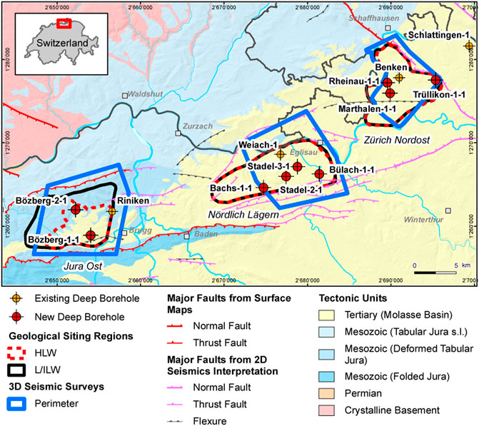
FIGURE 1. Tectonic map showing the drill sites of the studied boreholes.
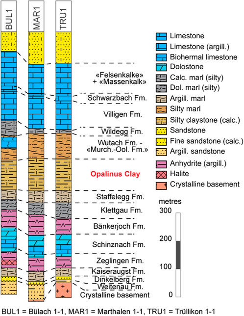
FIGURE 2. Lithostratigraphic profiles of the boreholes Bülach 1-1, Marthalen 1-1 and Trüllikon 1-1.
3 Methods
3.1 Medical X-ray computed tomography (Med-XCT)
Imaging of drill cores was performed with a Somatom Definition AS 64 Med-XCT equipment (Siemens, Forchheim, Germany). The acquired image stacks had a voxel size of 0.25 x 0.25 x 0.4 mm. Med-XCT provides qualitative information on density variation along drill cores. This method was often applied to geomaterials (e.g., Ashi, 1995; Ashi, 1997; Mees et al, 2003; Taud et al, 2005; Jovanovic et al, 2013; Gupta et al, 2018). Because qualitative information in the form of image gray values (CT values) is not satisfactory, previous studies have calibrated CT values to obtain a quantitative density distribution in geomaterials (Ashi, 1995; Gupta et al, 2018). Furthermore, Med-XCT is an imaging technique in which image resolution is related to sample size, and on the length scale of meters, the expected voxel size (i.e., resolution) is in the hundreds of micrometers. This length is much larger compared to typical grain and pore sizes in claystone. Therefore, the CT values of a particular image voxel indicates an “average” material density related to the volume fractions of various minerals filling the volume of that particular voxel.
Artifacts related to the beam hardening (BH) phenomenon were corrected according to the procedure described in Keller and Giger (2019). A short summary of the applied procedure is given here. BH is a phenomenon associated with the X-ray beam’s polychromatic nature related to the used med CT instrument. In the image data, the artifact is shown by the fact that in image planes perpendicular to the sample cylinder axis, the CT values depend on the radial distance between the cylinder axis and the circular edge of the sample. Thereby, the CT values systematically decrease towards the center of the sample. To remove the BH artefact, this systematic decrease was described by a polynomial function of second degree, which then allowed a BH correction to be applied for each image plane.
3.2 XCT technology and calibration of CT values with respect to major constituents
The incident X-ray intensity variation varies as function of the X-ray path length and the linear attenuation coefficient (LAC) of the target material. The LAC is a function of the chemical composition and the density of the target material. Grey levels in XCT images represent attenuation in each voxel. Grey levels, also termed CT values, in XCT images are scaled according to the Hounsfield (HU) scale, where air has HU = −1,000 and water has HU = 0. The XCT device used is calibrated daily for air. XCT image data are 3D arrays where each entry corresponds to the measured CT value at a specific location and in a specific volume (= voxel volume). Such volumetric grids can be visualized by a technique called volume rendering where every CT value is mapped to a color and an opacity, which results in the typical grey scale 3D images. In this study, this technique was used to visualize cross-sections along drill-core samples. However, most of this study uses XCT data in the form of 3D arrays of CT values and uses them to calculate the results presented.
The spatial distribution of CT values primarily reflects the density contrast in a material, which in turn is controlled by spatial variations in composition. From this follows the goal of computing a spatial distribution of composition from the given spatial distribution of CT values. This is only possible if the CT values are calibrated with respect to the composition. For the calibration, a data set consisting of laboratory measured rock compositions and porosity as well as average CT values was compiled. These CT values were obtained by averaging the CT values over the same sample volume that was used in the laboratory to determine the rock composition. This resulted in 227 composition/CT value pairs. Because each CT values reflects the composition in a volume, the laboratory data with units in wt% were converted to units of vol%. In addition to samples from Opalinus Clay the data set includes data points from the units above and below Opalinus Clay (Figure 2). Information about the stratigraphy of Opalinus Clay and adjacent formations can be found in Figure 2 as well as, for example, in Hostettler et al (2017). The bulk rock mineralogy was measured by the University of Bern, Switzerland. Identification of the mineral phases and quantification of their relative proportions was done by powder X-ray diffraction. Quantitative evaluation of the diffraction patterns is performed by the Rietveld method or by a combined Rietveld-Pawley approach if clay minerals are present in the sample (for more details see Waber, 2020).
Next, the influence of 10 components (contents of calcite, dolomite, siderite, quartz, albite, k-feldspar, pyrite, C-organic and clay minerals given in units of vol% and porosity), on the CT value was analyzed by performing a partial least squares regression (PLSR) that aims to predict the CT value from 2 PLS components (Rosipal and Krämer, 2006). The 2 PLS components are linear combinations of the original variables and are defined by the PLS weights. These weights describe how much each component in the PLSR depends on the original variables and in what direction (Figure 3A).
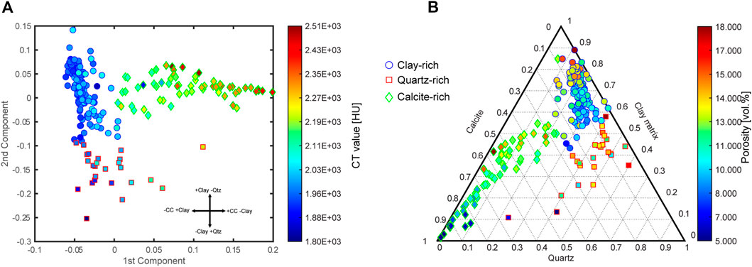
FIGURE 3. Analysis of the data used for the calibration of the CT values. (A) CT value plotted against the two partial least squares regression (PLSR) predictor variables where the symbol face color shows the CT value. The arrows indicate the influence of calcite (CC), quartz (Qtz) and clay minerals (Clay) on the value of the PLSR variables and on the CT value. The data were divided into three clusters (different symbols), which correspond to different sediment types. (B) Ternary plot with the end members calcite, quartz, and clay matrix, which together account for more than 80% of the rock volume. The color of the symbol faces indicates porosity. The plot illustrates the different composition of the three rock types (see text).
Figure 3 A shows a scatter plot in which the composition data are plotted as a function of the two PLS components. The procedure divides the data into three clusters, which differ in their composition. The PLS weights reveal that the value of the PLS components depends mainly on the volumetric content of calcite, clay minerals and quartz. Thus, the three clusters represent clay-rich, quartz-rich, and calcite-rich rock samples. The face color of the symbols shows the corresponding CT value, and it is obvious that the content of clay minerals, and quartz affects the CT value in the same way. It is also worth noting that with increasing calcite content, the CT value becomes higher. The data were also plotted in a ternary diagram with calcite, quartz, and clay matrix as end-members (Figure 3B). Because the pores occur predominantly in the clay-rich parts (Keller et al, 2011), the volumetric content of clay minerals and pores were combined. These three end-members account for more than 80% of the total rock volume and it is, therefore, fair to assume that the rock properties depend largely on the content of these end-members. The three composition groups can easily be distinguished in the ternary diagram. The face color of the symbols shows the porosity, and it is evident that in the calcite rich group the porosity increases with increasing clay content. The same is true for the clay-rich group. It should be noted that the correlations between clay content and quartz content in the individual composition groups are different, which can also be seen in the ternary diagram (Figure 3B). In the calcite-rich group the calculated correlation coefficient between clay content and quartz is 0.72 while in the clay-rich group it is-0.71. Since the composition groups have their own specific effect on the CT value and the relationship between mineral contents in the groups is different, a separate calibration between CT value and composition was calculated for each group to predict the rock composition for a given CT value.
Figure 4 shows the relationship between the CT value and the volumetric content of calcite, quartz, clay minerals and porosity for the three compositional groups. Linear relationships were fitted to the data that are used to predict individual compositional values from given CT values at specific locations along the drill cores. With respect to the prediction error of the linear models that are used to predict individual values, the relevant prediction interval is the one that tells us where effectively a certain fraction, for example, 80%, of the compositions for a given CT value will be found with 95% confidence (Wallis, 1951). This is precisely what is given by the tolerance intervals (black dashes lines) as shown in Figure 4. For example, in case of the clay content of the clay rich group we can be 95% sure that an interval of ∼± 10 vol% around the mean clay content predicted by the regression covers about 80% of the clay content values. Note, that the tolerance interval is much wider than the commonly used 95% confidence interval (red dashes lines) of the linear regression, which is a measure of the uncertainty of the expected mean value of a certain property and must not be confused with the prediction error related to an individual value.
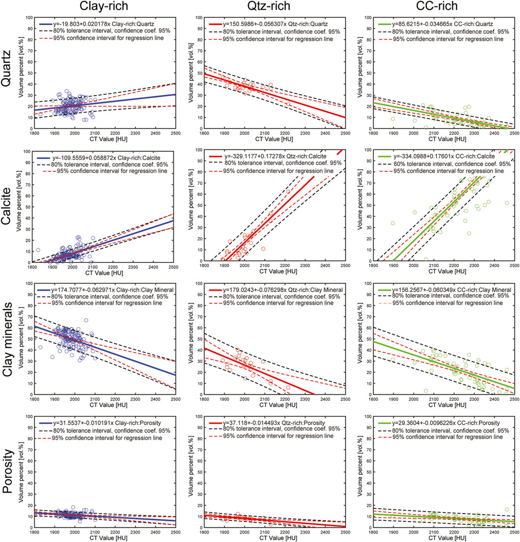
FIGURE 4. Calibration of CT values. Mineral contents and porosity in units of vol% plotted against CT values. The figure is organized so that the rows correspond to the mineral content and porosity and columns to the three rock types Symbols are measured values and the solid lines are the corresponding linear regressions.
The samples from the calcite-rich composition group were collected from the rock formations above and below Opalinus Clay (Figure 2). Quartz-rich samples occur in the upper part of Opalinus Clay as well as above and below of Opalinus Clay (Figure 2). To calculate the rock composition from image data, the respective calibration related to the three rock composition groups were used.
4 Uncertainties in determining effective properties of opalinus clay
4.1 Data reduction and conversion into 1D compositional profiles
A statistical analysis requires rock composition data over a large section of Opalinus Clay and at the highest possible resolution. Such data are available in the form of XCT image data in the form of the spatial distribution of CT values, which have a resolution in the submillimeter range. Therefore, the image stacks (i.e., 3D arrays of CT values) of the scanned samples were compiled in one matrix (i.e., as one column of rock) according to their depth. Considering the total amount of data would result in an enormous amount of data that cannot be handled. For each sample, the amount of data was reduced by storing the average CT value for all 2D arrays (= image planes) along the third dimension, which is perpendicular to the bedding plane. This is justified because the orientation of these image planes is parallel to the bedding and thus the variation in composition with respect to the lateral extent of the drill cores is negligible. For the visualization, a cross-section (= 2D array of CT values) through the sample parallel to the third dimension (= perpendicular to bedding) was stored. The analysis was done for the Bülach 1-1 borehole, for which the available data density is the highest and the Trüllikon 1-1 borehole. The data reduction results in one dimensional arrays of CT values oriented perpendicular to the bedding with the CT values 0.4 mm apart. The compiled data (Figures 5, 6) do not represent continuous columns of rock because they had not been sampled and scanned continuously. Using the calibration of CT values (Figure 4), the 1D arrays of CT values were converted into contents of calcite, quartz and clay minerals. This procedure was applied to 60 samples from Opalinus Clay of the Bülach 1-1 borehole corresponding to a length of 16.7 m distributed over the entire thickness of Opalinus Clay. The same was done for the 31 samples from Trüllikon 1-1 borehole, which corresponds to a length of 10.1 m. The resulting compositional profiles perpendicular to bedding are depicted in Figures 5, 6. The depth values in Figures 5, 6 correspond to the top of the samples.
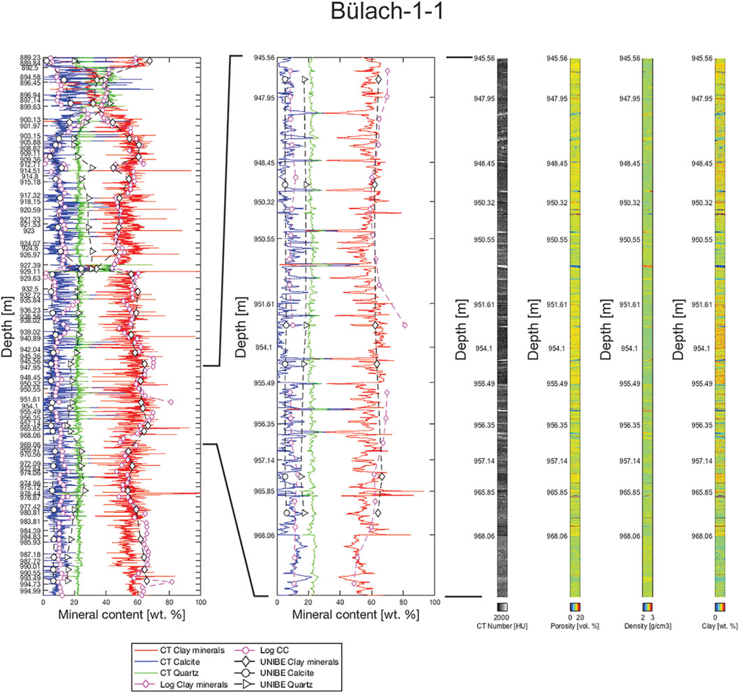
FIGURE 5. The X-ray images of the Bülach-1-1 borehole were compiled into virtual rock columns according to their depths. The CT values were converted into mineral contents (e.g., CT Clay minerals) based on the calibration (Figure 2) and displayed as composition profiles (far left). To compare CT based contents with the laboratory data (e.g., UNIBE calcite) and date from borehole logging (e.g., Log CC) they are given in units of wt%. One section is shown in more detail to illustrate the variation of cm to dm thick layers and their sequence (second from left). This includes 2D plots showing cross-sections through the rock column (four right columns). From left to right these show the distribution of: i) CT values, ii) porosity, iii) density and iv) clay mineral content.
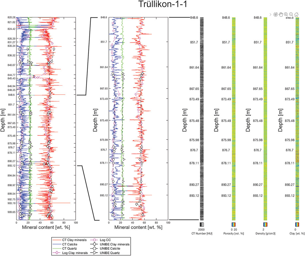
FIGURE 6. Same as Figure 3 but for the Trüllikon-1-1 borehole.
4.2 Representative sample length and number of samples
In the following, I address the question of whether the collected samples and related number of measured rock compositions allow the calculation of a representative average rock composition with an acceptable error that accounts for the composition of the Opalinus Clay at the 10-m scale. Another question that arises is the minimal length above which the rock composition behaves approximately homogeneously, which is particularly important for simulations that consider Opalinus Clay as a continuum. To answer this question, a statistical analysis is required, which in turn requires data sets on a systematic sampling of the rock column, whereby the sampling is performed with different sample lengths L in each case. Such a sampling was performed virtually on the 1D profiles, which represent rock columns, depicted in Figures 5, 6, measuring the volumetric content of quartz, calcite, and clay minerals for sample lengths L = 1, 5, 10, 25, 50, 75, and 100 cm. Sampling was performed from top to bottom as in reality. The distance between samples was randomly chosen between 20 and 30 cm. Such a method can be easily implemented in MATLAB, where subarrays of length L are extracted from a 1D array (=1D compositional profile) and their mean values are calculated and stored. Of course, the distance between the data points must be taken into account, which in this case is 0.4 mm. For each sample length L this procedure results in a data set consisting of n compositions for calcite, quartz, and clay minerals. The composition profiles were calculated based on the calibration (Figure 4) which is subject to a prediction error. However, during virtual sampling, a mean value is calculated for a given sample length L, which depends only little on the prediction error. This was tested by alternately adding or subtracting the prediction error from the predicted values along the profile, which results in a higher variance over the entire profile but not affecting the results of the sampling process.
After sampling, the representative sample length L can be defined for a physical property such as the volume fraction
where
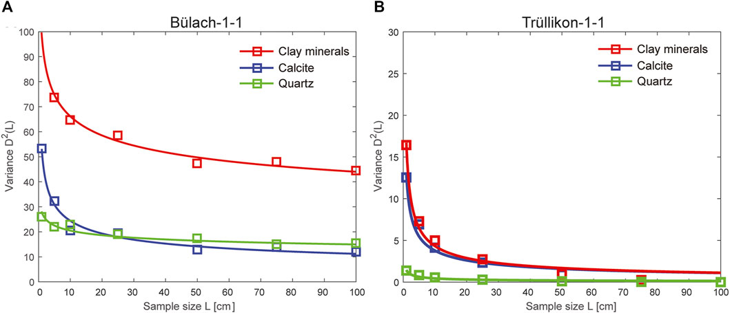
FIGURE 7. In a simulated sampling procedure applied to the virtual rock columns of Figure 3 and 4 (left), the figure shows the variance (symbols) of clay mineral content, calcite content and quartz content as a function of sample length. The lines correspond to a fit of Eq 2 to the data. (A) Bülach-1-1 borehole, (B) Trüllikon1-1 borehole.
This yielded the values for β and α.
After β and α were determined Eqs 1, 2 can be combined, which yielded an expression for the relative error as a function of sample length L and number n of samples.
5 Results
5.1 1D compositional profiles
UNIBE laboratory measurements and compositions related to borehole logging were also plotted along with the calculated composition profiles (Figures 5, 6). As for the general composition trend, the agreement between the laboratory data and the image-based data is reasonably good. Data from borehole logging deviate in some places (e.g., depth between ∼890 m and 903 m in Figure 5) from the laboratory data, which is particularly true for the Bülach 1-1 borehole. There were problems with borehole logging in this borehole and the composition was subsequently determined on the drill cores, which may be a reason for the discrepancies. However, an assessment of the logging quality is beyond the scope of this work. It is evident that in contrary to the image-based method, the laboratory measurements and logging data cannot resolve the decimeter-sized compositional variations.
5.2 Asymptotic decrease of variance with increasing sample length L
Figure 7 shows the variance (symbols) that was calculated form the data sets obtained by virtual sampling and the associated fit of Equation (2). The following applies for both boreholes, if the sample length L exceeds 30–40 cm, the variance for all three major components decreases only slightly with increasing L. In addition, the variance is lower for Trüllikon-1-1 than for Bülach-1-1. For sample lengths L > 30–40 cm, the variance is comparatively small for Trüllikon-1-1.
5.3 Representative sample length and number of samples
Figure 6 shows the expected error in the determined average content of calcite, quartz, and clay minerals as a function of sample length L and in case of measuring 1, 2, 10, and 30 samples. The error is largest for the determination of the average content of calcite and over 30 samples with a length L > 10 cm must be measured to reduce the error to an acceptable level. In the case of Bülach 1-1, taking a single sample with a length of 10 m produces still a comparable high error. Note that 30 samples taken with increasing depth with a total length of <10 m yields an average composition with a much lower error when compared to a single sample with the length of 10 m. Hence it follows that the distribution of cm to dm thick layers, which are enriched in calcite, is variable over the whole thickness of Opalinus Clay and that a minimum and handleable sample length above which Opalinus Clay behaves homogeneously does not exist. This may be important for safety issues addressed via calculations and simulations that consider Opalinus Clay as a continuum. For such applications, a sufficiently large number (n > 30) of samples must be considered to determine the effective properties of Opalinus Clay.
Of interest is whether enough samples were collected and measured during the deep drilling campaign to account for compositional variations along the rock column. The laboratory measurements of rock composition related to Opalinus Clay from the Bülach 1-1 and Trüllikon 1-1 boreholes were determined from samples approximately 25 cm in length. For these laboratory-based data sets, the relative error was calculated according to Eq. 1 and is presented in Table 1. This table also presents the relative errors obtained by the statistical analysis using the same sample length and number of samples. The agreement is considered good and confirms that the method of image based virtual sampling and subsequent statistical analysis can be used to predict how representative a planned sampling strategy is. In addition, Table 1 implies that the composition at the Trüllikon location is more homogeneous than in Bülach, as also shown by Figures 7, 8.

TABLE 1. Comparison between the relative error calculated from i) the laboratory data (Lab) and ii) resulting from the statistical analysis (Stat). The number of samples are the number laboratory measurements that are plotted in Figures 3, 4.
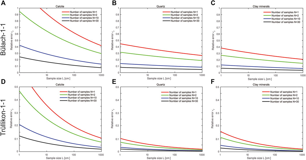
FIGURE 8. The relative error of the mean mineral content of a sample as a function of its length. (A) Calcite, (B) Quartz and (C) Clay mineral content related to Bülach-1-1 borehole. (D) Calcite, (E) Quartz and (F) Clay mineral content related to Trüllikon-1-1 borehole.
6 Discussion
6.1 Rock composition prediction from X-ray images
The major advantage of X-ray imaging over other methods in evaluating the composition along drill cores is the higher resolution (Figures 5, 6). Using X-ray imaging, the layer structure of Opalinus Clay can be resolved, which was not possible with laboratory analyses and geophysical borehole logging with a measuring interval of 20 cm. Laboratory measurements and logging result in a smoothing of the true compositional profile along the rock unit. Hence, these methods do not reflect the true nature of the Opalinus Clay and lead to a misleading picture. The disadvantage of X-ray imaging is the high effort to measure significant portions of the whole rock column of a borehole.
The problem with predicting rock compositions from CT values is that the result is not unique because different mineral combinations can produce the same CT value. This is especially true in fine-grained rocks where each voxel volume is filled by several mineral grains. However, the study shows that the prediction works well within certain compositional ranges related to different rock types where each rock type has its own effect on CT values. For the application, each rock type requires a separate calibration of the CT values. The problem is simplified by the fact that in the sedimentary rocks studied, the CT value is mainly governed by the content of calcite, quartz, clay minerals and pores. These four components make up more than 80% of the rock volume and are expected to substantially influence the rock properties. The number of components can further be reduced if clay minerals and pores are combined as a single component. That this is justified was shown microstructurally on the pore scale (Keller et al, 2011) but it is also reflected by a positive correlation between clay mineral content and porosity. Thus, the petrophysical properties of Opalinus Clay are determined by the respective volumetric content of three components: the clay matrix, carbonates, and quartz. The point here is that it is the volumetric fractions and not the weight fractions that determine the properties. The rock types were separated based on their influence on the CT value, but it is evident that they occur systemically in the rock column.
Apart from accessory minerals, the composition of Opalinus Clay and the calcite-rich rocks adjacent to Opalinus Clay are controlled by the behavior of one of the three major components (Figure 3B). In both composition groups, an increase in clay matrix or calcite leads to a decrease in the remaining two major components. In the quartz-rich rocks at top of Opalinus Clay, the relationships are ambiguous. What is also noticeable is that with comparable clay matrix content, the calcite-rich rocks as well as the quartz-rich rocks have a higher porosity than the clay-rich rocks (Figure 3B). This is most likely because the clay matrix in the clay-rich rocks is more compacted than in the other two rock types and quartz and calcite are present in almost clay-free layers or that calcite and quartz are present in the form of a cement.
Furthermore, the CT image analysis indicates that the composition of Opalinus Clay at the Trüllikon 1-1 site is more homogeneous compared to the Bülach 1-1 site. This is already evident from the comparison of the profiles in Figures 5, 6 and then recorded quantitatively in Figure 7 where the variance in composition is lower at the Trüllikon 1-1 site.
6.2 Effective properties of opalinus clay
For the prediction of the repository behavior, simulations are often used and consider the host rock as a continuum and assign certain effective properties to it. Bearing in mind the presented variability in the layer structure (Figures 5, 6), the general question arises about what effective properties Opalinus Clay has on the scale of a repository. In this context, the concept of a representative volume element (RVE) comes into play, which is generally considered the minimum volume for which Opalinus Clay is expected to behave homogeneously in regard of the property of interest. As far as the composition is concerned, it was shown here that such a minimum volume does not exist in the sense that the measurement of a sufficiently large and handleable volume yields a composition that satisfyingly represents the bulk composition of Opalinus Clay unit. The cause is the inhomogeneous distribution and variation of the cm to dm thick layers. This phenomenon occurs over the entire thickness (see also Lauper et al, 2018) and was here documented by X-ray imaging. An alternative is the determination of a mean composition with an acceptable error based on a certain number of collected samples (Kanit et al, 2003). Thereby, virtual sampling provides insight into the variance of bulk rock composition as a function of sample length. Such information helps to optimize the sampling procedure on the basis of which a representative mean bulk composition can be determined. For example, in case of the Bülach 1-1, the variance of the bulk calcite content decreases by 70% when the sample length increases from 1 cm to 30 cm. A further increase from 30 cm to 100 cm leads to a further decrease in the variance of only 10%. Hence, if sampling is done continuously from top to bottom at a certain interval, the cost-efficient sample length is around 30 cm. This length ensures sampling of a reasonable number of different layer sequences during the sampling procedure. For this sample length, approximately 30 samples must be collected and measured in order that the relative error related to bulk mean calcite content decreases to an acceptable level of around 15%.
7 Conclusion
X-ray imaging is a comparatively inexpensive method compared to other methods used in a deep drilling campaign. X-ray imaging of drill cores provides data on the compositional variation on the mm scale. Other methods such as borehole logging measure composition at intervals of a few dm. The composition of Opalinus Clay varies on the cm to dm scale, and this variation is coupled to a layered structure in which the layers vary in composition. Hence, methods that measure the composition in dm intervals cannot account for the true nature of Opalinus Clay. For predicting the behavior of the repository of nuclear waste by simulations, the host rock is usually considered as a continuum. Thereby, the assignment of the effective properties is complicated by the variable layer structure. The effective properties must be determined in the form of average values associated with the smallest possible error. In the case of bulk rock composition, this is done by repetitive measurement of samples with an ideal length of 30 cm. At least 30 samples distributed over the entire thickness of Opalinus Clay must be measured to account for the variance in layer sequence.
Data availability statement
The raw data supporting the conclusion of this article will be made available by the authors, without undue reservation.
Author contributions
The author confirms being the sole contributor of this work and has approved it for publication.
Funding
This work was funded by the Swiss National Cooperative for the Disposal of Nuclear Waste (NAGRA). Open access funding by Zurich University of Applied Sciences (ZHAW).
Acknowledgments
The author would like to thank Nicole Schwendener for her help with the medical x-ray apparatus and scanning of the samples.
Conflict of interest
The authors declare that the research was conducted in the absence of any commercial or financial relationships that could be construed as a potential conflict of interest.
Publisher’s note
All claims expressed in this article are solely those of the authors and do not necessarily represent those of their affiliated organizations, or those of the publisher, the editors and the reviewers. Any product that may be evaluated in this article, or claim that may be made by its manufacturer, is not guaranteed or endorsed by the publisher.
References
Andra, (2005). Dossier 2005 Argile – evaluation de la faisabilité du stockage géologique en formation argileuse profonde – rapport de synthèse. Available at: http.//www.Andra.fr (Juin 2005. Andra, France).
Ashi, J. (1997). “Computed tomography scan image analysis of sediments,” in Proceedings of the ocean drilling program, scientific results. Editors T. H. Shipley, Y. Ogawa, P. Blum, and J. M. Bahr (Texas, United States: Texas A&M University), 151–159.
Ashi, J. (1995). “CT scan analysis of sediments from Leg 146,” in Proceedings of the ocean drilling program, scientific results. Editors B. Carson, G. K. Westbrook, R. J. Musgrave, and E. Suess (Texas, United States: Texas A&M University), 191–199.
Bläsi, H.-R., Peters, T., and Mazurek, M. (1991). Der Opalinus-Ton des Mt. Terri (Kanton Jura): Lithologie, Mineralogie und phyiko-chemische Gesteinsparameter. Wettingen, Switzerland: Nagra, Wettingen. Nagra Interner Bericht, NTB 90-60.
Gupta, L. P., Tanikawa, W., Hamada, Y., Hirose, T., Ahagon, N., Sigihara, T., et al. (2018). Expedition NGHP, 02 JAMSTEC Science Team Examination of gas hydrate-bearing deep ocean sediments by X-ray computed tomography and verification of physical property measurements of sediments. Mar. Pet. Geol. 108, 239–248. doi:10.1016/j.marpetgeo.2018.05.033
Hostettler, B., Reisdorf, A. G., Jaeggi, D., Deplazes, G., Bläsi, H.-R., Morard, A., et al. (2017). Litho- and biostratigraphy of the Opalinus Clay and bounding formations in the Mont Terri rock laboratory (Switzerland). Swiss J. Geosci. 110, 22–37. doi:10.1007/s00015-016-0250-3
Jeulin, D. (2012). Morphology and effective properties of multi-scale random sets: A review. C. R. Mec. 340, 219–229. doi:10.1016/j.crme.2012.02.004
Jovanovic, Z., Khan, F., Enzmann, F., and Kersten, M. (2013). Simultaneous segmentation and beam-hardening correction in computed microtomography of rock cores. Comput. Geosci. 56, 142–150. doi:10.1016/j.cageo.2013.03.015
Kanit, T., Forest, S., Gailliet, I., Mounoury, V., and Jeulin, D. (2003). Determination of the representative volume for random composites: Statistical and numerical approach. Int. J. Solids Struct. 40, 3647–3679. doi:10.1016/S0020-7683(03)00143-4
Keller, L. M., and Giger, S. B. (2019). Petrophysical properties of Opalinus clay drill cores determined from med-XCT images. Geotech. Geol. Eng. 37, 3507–3522. doi:10.1007/s10706-019-00815-2
Keller, L. M., Holzer, L., Wepf, R., and Gasser, P. (2011). 3D geometry and topology of pore pathways in Opalinus clay: Implications for mass transport. Appl. Clay Sci. 52, 85–95. doi:10.1016/j.clay.2011.02.003
Keller, L. M., Schwiedrzik, J. J., Gasser, P., and Michler, J. (2017). Understanding anisotropic mechanical properties of shales at different length scales: In situ micropillar compression combined with finite element calculations. J. Geophys. Res. Solid Earth. 122. doi:10.1002/2017JB014240
Lauper, B., Jaeggi, D., Deplazes, G., et al. (2018). Multi-proxy facies analysis of the Opalinus Clay and depositional implications (Mont Terri rock laboratory, Switzerland). Swiss J. Geosci. 111, 383–398. doi:10.1007/s00015-018-0303-x
Matter, A., Peters, T., Bläsi, H.-R., Meyer, J., Ischi, H., and Meyer, C. (1988). Sondierbohrung weiach—geologie. Nagra technischer bericht, NTB 86-01. Wettingen, Switzerland: Nagra, Wettingen.
Matter, A., Peters, T., Isenschmid, C., Bläsi, H.-R., and Ziegler, H.-J. (1987). Sondierbohrung riniken—geologie. Nagra technischer bericht, NTB 86-02. Wettingen, Switzerland: Nagra, Wettingen.
Mees, F., Swennen, R., Van Geet, M., and Jacobs, P. (2003). Applications of X-ray computed tomography in the geosciences Geological Society. London, United Kingdom: Special Publications, 1–6.
Nagra, (2014). Beurteilung der Tiefenlage in Bezug auf die geotechnischen Bedingungen: Grundlagen für die Abgrenzung und Bewertung der Lagerperimeter. Nagra Arbeitsbericht. Wettingen, Switzerland: Nagra, Wettingen. NAB 14-81.
Nagra, (2002). Projekt Opalinuston: Synthese der geowissenschaftlichen Untersuchungsergebnisse. Entsorgungsnachweis für abgebrannte Brennelemente, verglaste hochaktive sowie langlebige mittelaktive Abfälle. Nagra Technischer Bericht, NTB 02-03. Wettingen, Switzerland: Nagra, Wettingen.
Nagra, (2001). Sondierbohrung benken untersuchungsbericht. Nagra technischer bericht, NTB 00-01. Wettingen, Switzerland: Nagra, Wettingen.
Rosipal, R., and Kramer, N. (2006). “Overview and recent advances in partial least squares,” in Subspace, Latent Structure and Feature Selection: Statistical and Optimization Perspectives Workshop (SLSFS 2005), Revised Selected Papers (Lecture Notes in Computer Science 3940), Bohinj, Slovenia, February 23-25, 2005, 34–51.
Taud, H., Martinez-Angeles, R., Parrot, J. F., and Hernandez-Escobedo, L. (2005). Porosity estimation method by X-ray computed tomography. J. Pet. Sci. Eng. 47, 209–217. doi:10.1016/j.petrol.2005.03.009
Waber, H. H. (2020). SGT-E3 deep drilling campaign (TBO): Experiment procedures and analytical methods at RWI. Bern, Switzerland: University of Bern. Nagra Arbeitsbericht NAB 20-13 (Version 1.0, April 2020.
Wallis, W. A. (1951). “Tolerance intervals for linear regression,” in Second Berkely symposium on mathematical statistics and probability. Editor J. Neyman (Los Angelos, United States: University of California Press), 43–51.
Keywords: opalinus clay, nuclear waste, deep drilling, effective properties, compositional variations
Citation: Keller LM (2023) XCT analysis of drill cores of Opalinus clay and determination of sample size for effective properties evaluation. Front. Earth Sci. 11:1177408. doi: 10.3389/feart.2023.1177408
Received: 01 March 2023; Accepted: 19 May 2023;
Published: 30 May 2023.
Edited by:
Ángel Puga-Bernabéu, University of Granada, SpainReviewed by:
Anxo Mena, Centro Tecnológico del Mar (CETMAR), SpainLallan P. Gupta, Japan Agency for Marine-Earth Science and Technology (JAMSTEC), Japan
Copyright © 2023 Keller. This is an open-access article distributed under the terms of the Creative Commons Attribution License (CC BY). The use, distribution or reproduction in other forums is permitted, provided the original author(s) and the copyright owner(s) are credited and that the original publication in this journal is cited, in accordance with accepted academic practice. No use, distribution or reproduction is permitted which does not comply with these terms.
*Correspondence: Lukas M. Keller, kelu@zhaw.ch