Mapping structural lineaments using the edge filters of the potential field: a case study of the Rizhao–Lianyungang area, East China

Background: Edge enhancement plays an important role in potential field data processing and interpretation, which facilitate regional tectonic studies, mineral and energy exploration. This is because edges on potential field often indicate linear geological structures such as fractures, edges of geological bodies and so on. With the development of meticulous edge enhancement on potential field, the phenomenon of false edges caused by the associated anomalies when detect ing edges from magnetic field cannot be ignored.

Methods: Aiming at this problem, we proposes a modified magnetic edge detection method (SP Mag) based on the second order spectral moment. This method has been tested on both synthetic and field data. The synthetic test show that SP Mag cannot only balanced edges no matter from strong or weak anomalies, but also eliminates those false edges caused by the associated anomalies in magnetic field, which provide more effective information for subsequent interpretation.

Results: We apply this new method to the RTP aero magnetic field and gravity field of Rizhao Lianyungang area. The lineaments recognized by the SP Mag method correspond well with geologic structures through comparing with geological maps.

Discussion: The results illustrate the usefulness of the method for potential field interpretation. Furthermore, more geological and geophysical data should be still combined for comprehensive interpretation in the actual interpretation, though the SP Mag method can recognize lineaments effectively.

1 Introduction

Edges detected from the potential field often correspond to geological linear structures such as faults, geological contracts, and sources’ boundaries, which can play an important role in geotectonic research, energy and mineral exploration, etc. Therefore, developing many edge-enhancing methods is highly desired. Edge enhancement in the early stage is mainly based on horizontal and vertical derivatives. For example, these high-pass filters include vertical derivatives (Evjen, 1936), horizontal gradient (HGA) (Cordell, 1979; Fedi and Florio, 2001), fitting paraboloid on the horizontal gradient (Blakely and Simpson, 1986), and analytic signal methods (Nabighian, 1972; Roest, 1992; Hu et al., 1995; Guan and Yao, 1997). As is known, methods based on horizontal and vertical derivatives often detect boundaries of sources with lager amplitude well but not very effective for edges of small-amplitude sources (Sun et al., 2016a). Therefore, the tilt angle method (Miller and Singh, 1994) was proposed to balance different amplitude anomalies, which was the first balanced filter. However, it is not an edge-detection method. Then, the balanced edge-enhancing methods emerge endlessly, such as the total horizontal derivative of the tilt angle (Verduzco et al., 2004), theta map (Wijins et al., 2005), calculating the tilt angle on the total horizontal derivative (Francisco et al., 2013), and the curvature of the total horizontal gradient amplitude (Hansen and de Ridder, 2006; Phillips et al., 2007). In order to detect more details but with less noise interference, numerous excellent edge-enhancing filters are proposed (Cooper and Cowan, 2008; Cooper, 2009; Cooper and Cowan, 2011; Wang et al., 2013), for example, the normalized standard deviation (NSTD), the orthogonal Hilbert transforms of analytic signal amplitudes, and the generalized derivative operator. On the basis of NSTD, the normalized anisotropy variance method was developed by Zhang et al. (2014) to recognize linear structures and meanwhile suppress noise. Ma et al. (2012) proposed balancing filters and enhanced local-phase filters to detect edges, which showed higher resolution and less sensitivity to noise than the theta map method. Hu et al. (2019) presented the normalized facet edge-detection method to enhance weak and noisy signals produced by shallow and deep mass anomalies. Pham et al. (2020a), Pham et al. (2020b), and Pham et al. (2021) proposed some excellent filters, of which the application for interpreting geological structures showed that it can balance edges from both strong and weak anomalies avoiding producing the spurious edges (Pham et al., 2021; Eldosouky et al., 2022). For example, the method based on an arcsine function uses the ratio of the vertical gradient to the total gradient of the amplitude of the horizontal gradient field (EHGA) (Pham et al., 2020b), the improved logistic (IL) filter (Pham et al., 2020a), and the enhanced total gradient (ETG) method (Prasad et al., 2022).

Our previous work has proposed an edge-enhancing method based on the second-order spectral moment (SP-Gra for short) on the potential field (Sun et al., 2016a). Both synthetic data and real data experiments show that it has strong ability on weak boundary enhancing and spatial discrimination. With the deepening of research, we find that many “false edges” are also outlined, producing false information for the following interpretation. This is because the relationship between magnetic anomaly and susceptibility is much more complicated than the positive correlation between gravity anomaly and density. The center of a perpendicularly magnetized magnetic anomaly is generally positive to the magnetic susceptibility, but there often exist associated anomalies opposite to magnetic susceptibility anomalies (Figures 2B, C). If we apply the SP-Gra method, both the main boundaries of anomalies and associated anomalies can be detected simultaneously. In addition, the boundaries of the associated anomaly are the “false edges.” In fact, in addition to the SP-Gra method, many edge-enhancing methods (e.g., NSTD method) also outline the “false edges,” and the stronger the edge-enhancing ability is, the more obvious the “false edges” detected are. If these “false edges” caused by associated anomalies are not eliminated, false information will be provided for later geological interpretation.

In this paper, we propose a modified magnetic edge-detection method on the basis of Poisson’s formula aiming at edge detection from the magnetic field, which is named the SP-Mag method. It can balance the boundaries of sources with both high and low amplitudes well and then the recognized boundaries when detecting edges from the magnetic field. Furthermore, it can also eliminate false edges produced by the associated anomalies, meanwhile providing more accurate information for the later geological interpretation.

2 Magnetic edge enhancements using the second-order spectral moment

2.1 The gradient norm of the pseudo-gravity field

Geophysical potential fields include gravity and magnetic fields, but they show different features (Zeng et al., 2018). As is well known, there is a more complicated relationship between magnetic field and magnetic susceptibility than that between gravity field and density. In addition, the magnetic field can be mathematically related to the pseudo-gravity through Poisson’s formula (Zeng et al., 2018), which is

$U=k\cdot \nabla V.(1)$

Here, $k=-\frac{M}{4\pi G\rho }$, where k is a constant, M is the geomagnetic field intensity, and ρ is the equivalent density difference; U is the magnetic potential; and V is the pseudo-gravity potential field.

From Eq. 1, the magnetic scalar potential field that is vertically magnetized equals to the pseudo-gravity field

$U_{\perp }=k\cdot \frac{\partial V}{\partial z}=k\cdot g,(2)$

where g is the pseudo-gravity field.

$\left\{\begin{array}{l}k\frac{\partial g}{\partial x}=\frac{\partial U_{\perp }}{\partial x}=Ha{x}_{\perp },\\ k\frac{\partial g}{\partial y}=\frac{\partial U_{\perp }}{\partial y}=Ha{y}_{\perp }.\end{array}\right.(3)$

The total horizontal derivative of g is defined as

$B=\left|k\right|\sqrt{{\left({\partial }_{x}g\right)}^2+{\left({\partial }_{y}g\right)}^2}=\sqrt{Ha{x_{\perp }}^2+Ha{y_{\perp }}^2.}(4)$

From this formula 1, one can see that the ridges of $B\left(x,y,z=z_0\right)$ correspond to the edges of $g\left(x,y,z=z_0\right)$. In addition, we use the idea of the pseudo-gravity field, but there is no need to calculate it at all. Instead, we calculate two horizontal components, Hax and Hay, of the magnetic anomaly.

2.2 The edge coefficient

According to random process theory (Thomas, 1982), the (p + q)th order discrete spectral moment of a surface is (Sun et al., 2016a; Sun et al., 2016b)

$m_{pq}={\displaystyle \sum _{v=1}^n}{\displaystyle \sum _{u=1}^m}G\left(f_u,f_v\right){f_u}^p{f_v}^q\Delta f_u\Delta f_v,(5)$

where G (f_u,f_v) represents the two-dimensional power spectral density; f_u and f_v represent the discrete x- and y-directional spatial frequencies, respectively; and m and n are the sizes of the surface.

When sliding a moving window (w₁) point by point on the surface B, the three elements’ spatial expressions of the second spectral moment of the small windowed surface can be calculated by the derived formula (Yang et al., 2015; Sun et al., 2016b; Yang and Sun, 2016; Yang et al., 2017; Sun et al., 2022), which are

$\left\{\begin{array}{l}{m}_{20}={\displaystyle \sum _{i=1}^{N_{\alpha }}}{\displaystyle \sum _{j=1}^{M_{\alpha }}}{\left({\partial }_{x}B\left(x_j,y_i\right)\right)}^2,\\ m_{02}={\displaystyle \sum _{i=1}^{N_{\alpha }}}{\displaystyle \sum _{j=1}^{M_{\alpha }}}{\left({\partial }_{y}B\left(x_j,y_i\right)\right)}^2,\\ m_{11}={\displaystyle \sum _{i=1}^{N_{\alpha }}}{\displaystyle \sum _{j=1}^{M_{\alpha }}}{\partial }_{x}B\left(x_j,y_i\right){\partial }_{y}B\left(x_j,y_i\right),\end{array}\right.(6)$

where B (x_j, y_i) is the total horizontal derivative of pseudo-gravity within the sliding window w₁; i = 1,2, … N_α; j = 1,2, … M_α.

From Eq. 6, one can see that if the coordinates rotate, the spectral moments will change. Therefore, one can define the statistically invariable quantities (M₂ and △₂) independent of the system rotation, which are (Sun et al., 2016a, Yang et al., 1992; Huang, 1985; Thomas, 1982)

$M_2=m_{20}+m_{02},(7)$

${\Delta }_2=m_{20}{m}_{02}-m_{11}^2.(8)$

Here, M₂ represents the variance of the two-dimensional slope of B in the window w₁, showing the edges’ magnitudes. △₂ indicates the anisotropy of surface B in the window w₁.

In order to bring more details of small anomalies, the edge coefficient is defined as (Sun et al., 2016a; Li et al., 2000)

$\Lambda =-sign\left({\nabla }^{2}B\right)\cdot \frac{2\sqrt{{\Delta }_2}}{M_2}.(9)$

Here, ${\nabla }^2$ is the Laplacian operator. $\frac{\sqrt{{\Delta }_2}}{M_2}$ increases sharply near the maximum or minimum values of the scalar field B. When ${\nabla }^{2}B>0$, they correspond to the minimum values (valleys); when ${\nabla }^{2}B<0$, they correspond to the maximum values (ridges). From the aforementioned analysis, the ridges of B (x, y, z=z₀) correspond to the edges of g (x, y, z = z₀). Therefore, values of ∧>0 reflect the anisotropy of surface B (x, y, z = z₀) or edges of the surface of the pseudo-gravity field g (x, y, z = z₀).

The key of the SP-Mag method to eliminate false edges caused by the associated anomalies is that we define the variable B (formula 4) and modify the integral kernel by the variable B of m₀₂, m_11, and m₂₀ which are the most basic elements of the second-order spectral moment. This also shows the difference between the SP-Mag and SP-Gra (Sun et al., 2016a) methods. Furthermore, though we use the Poisson formula to derive and construct B, there is no need to calculate the pseudo-gravity field at all, which can avoid losing details caused by truncation errors.

3 Tests on synthetic data

We test the proposed SP-Mag method on two synthetic magnetic datasets without and with noise. Figures 1A, B display the 3D and ground view of the first simple model that consists of three prisms. The plan view of the model consisting of three cuboids A, B, and C is shown in Figure 2A. Cuboid A is with the size of 10 km × 1 km × 2 km and with a buried depth of 1.5 km; cuboid B is with the size of 1 km × 6 km × 1 km and with a buried depth of 1 km; and cuboid C is with the size of 1 km × 2 km × 0.5 km and with a buried depth of 0.5 km. The magnetic intensities of cuboids A, B, and C are 0.6, 1, and 0.02 A/m, respectively. We compute the synthetic data on a grid of 20 km × 25 km with 0.05-km spacing.

FIGURE 1

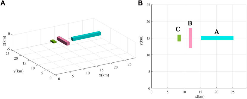
FIGURE 1. 3D view (A) and top view (B) of the first simple magnetic model.

FIGURE 2

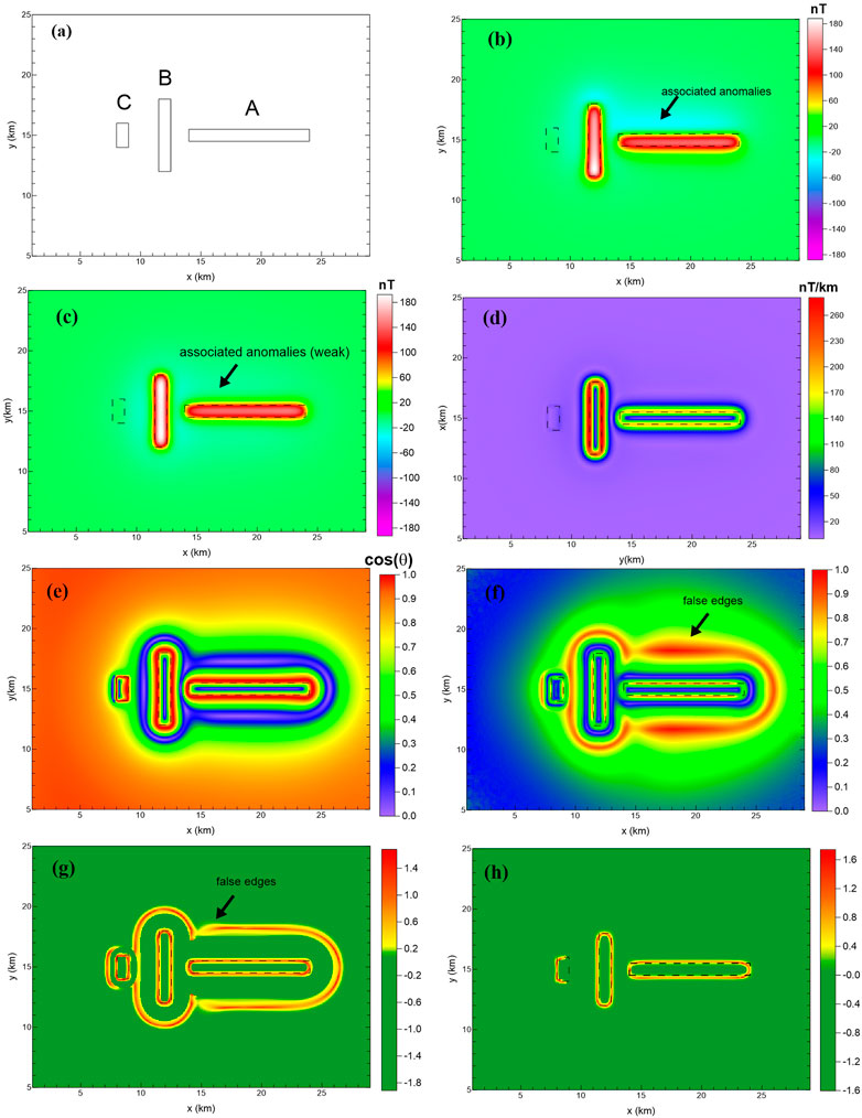
FIGURE 2. Comparison of the edge-enhancing methods. (A) Plane graph of the model; (B) synthetic magnetic anomaly of the model in Figure 1; (C) RTP magnetic anomaly; edge-detection results outlined from the RTP magnetic anomaly using (D) HGA; (E) theta map; (G) SP-Gra; and (H) SP-Mag.

The magnetic anomalies are calculated by the 3D forward modeling algorithm (Guan, 2005), and Figure 2Bshows the magnetic anomaly under oblique magnetization with the declination of 0° and inclination of 60°. There are two kinds of anomalies: the strong positive anomalies and the weaker negative anomalies. In addition, the weaker negative anomaly is the associated anomaly (indicated by the black arrow). The RTP (reduced to the pole) magnetic anomaly is shown in Figure 2C. Compared to Figure 2B, the RTP magnetic anomaly can not only reduce the positional deviation between the magnetic source and magnetic anomaly caused by the oblique magnetization but also suppress the associated anomalies. However, from Figure 2C, one can also see that the RTP magnetic anomaly can suppress associated anomalies but cannot eliminate them (indicated by the arrow in Figure 2C).

For comparison, we present edge-detection results outlined from the RTP magnetic anomaly (Figure 2C) using HGA, theta map, NSTD, and SP-Gra (Figures 2D–G, respectively). The HGA method (Figure 2D) can effectively identify the edges of prisms A and B with strong anomalies, while the boundary of prism C with the weaker anomaly has not been effectively identified. The theta map, NSTD, and SP-Gra methods have strong ability to enhance the weak boundary, so the boundaries of prisms A, B, and C are all well recognized. However, as the methods’ ability to enhance the weak boundary becomes stronger, the false boundaries (pointed by the arrow) caused by the associated anomaly gradually become prominent, which could interfere with the final interpretation.

Figure 2H shows the edges detected by the SP-Mag method that is proposed in this paper. Compared with HGA (Figure 2D), the SP-Mag method has a strong ability to enhance the weak boundary, so that edges detected from prism C with the weak magnetic anomaly are at the same magnitude as the edges detected from prisms A and B. Compared with the results of the theta map (Figure 2E), NSTD (Figure 2F), and SP-Gra (Figure 2G), the SP-Mag method has a good ability to eliminate the false edges caused by the associated anomalies. One can also observe that the boundary of prism C on the right side has not been recognized. This is because the definition of B (the total horizontal derivative of g in formula 4) is one order lower than the magnetic field, and the detected details are not as clear as the magnetic field.

In fact, the SP-Mag method is modified from the SP-Gra method. Thus, the SP-Mag method maintains the weak-edge-enhancing ability while eliminating the false edge caused by the magnetic field-associated anomalies, which can provide a more effective reference map for the subsequent interpretation. It is worth noting that when we apply the SP-Mag method, we do not need to compute the pseudo-gravity field at all but calculate two horizontal components of the magnetic anomaly—Hax and Hay (see Eqs 3, 4 for details) so that the problem of detail loss caused by the truncation error can be avoided.

In order to test the sensitivity of methods to noise, we add random noise to the synthetic magnetic anomaly, as shown in Figure 2B. The random noise has the amplitude of 0.5% of the maximum data magnitude. The magnetic anomaly with noise and the RTP is shown in Figures 3B, C, respectively. The results detected from the RTP magnetic anomaly with noise, as shown in Figure 3C, using HGA, theta map, NSTD, and SP-Gra methods are shown in Figures 3D–G. The HGA, theta map, and NSTD methods can identify the edges of prisms A and B, but the boundary of prism C cannot be effectively identified because of the influence of noise.

FIGURE 3

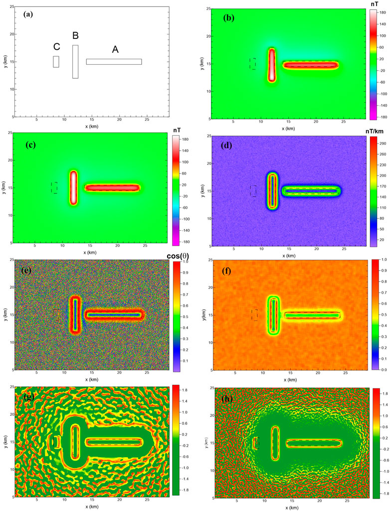
FIGURE 3. Edges detected by the methods. (A) Plane graph of the model; (B) synthetic magnetic anomaly, with an added noise of amplitude 0.5% of the maximum data magnitude; (C) RTP magnetic anomaly with noise; edge-detection results outlined from the RTP magnetic anomaly with noise using (D) HGA; (E) theta map; (F) NSTD; (G) SP-Gra; and (H) SP-Mag.

The SP-Gra methods can suppress noise, and the boundaries of prisms A and B, as well as the boundaries of prism C, can be recognized basically. The “false edges” affected by the noise become faintly visible. Because the SP-Gra method has a similar theoretical definition and calculation process to the SP-Mag method and both methods are based on the second-order spectral moment, the SP-Mag method has the similar ability to suppress noise. In addition, the SP-Mag method (Figure 3H) recognized the edges of prisms A and B and basically identified the edges of prism C except for the edges on the right side.

Figures 4A, B display the 3D and ground view of the second magnetic model that consists of two bodies (M1 and M2) with the same size but different depths, two overlapped sources (M3 and M4), and one thin source (M1). The geometric and magnetic parameters are shown in Table 1. The magnetic anomalies (Figure 5A) of the model are computed on a grid of 200 km × 160 km with 0.25-km spacing. Figure 5B shows the edges estimated by the HGA method. One can see that the results are dominated by the edges from the stronger source anomalies. Figures 5C, D show the edges estimated by the theta map and NSTD method, respectively. We can see that the two filters produce many false edges around and above the sources, and the theta map filter does not exhibit sharp peaks over the sources edges. Figures 5C, D show the results of the SP-Gra and SP-Mag filters. Both SP-Gra and SP-Mag filters provide the results with high resolution, but SP-Mag has the ability to avoid false edges in the map.

FIGURE 4

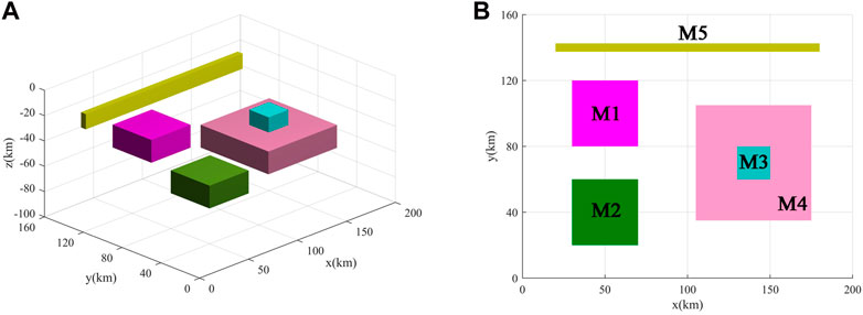
FIGURE 4. 3D view (A) and top view (B) of the second magnetic model.

TABLE 1

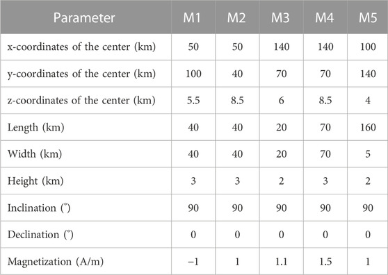
TABLE 1. Parameters of the second synthetic magnetic model.

FIGURE 5

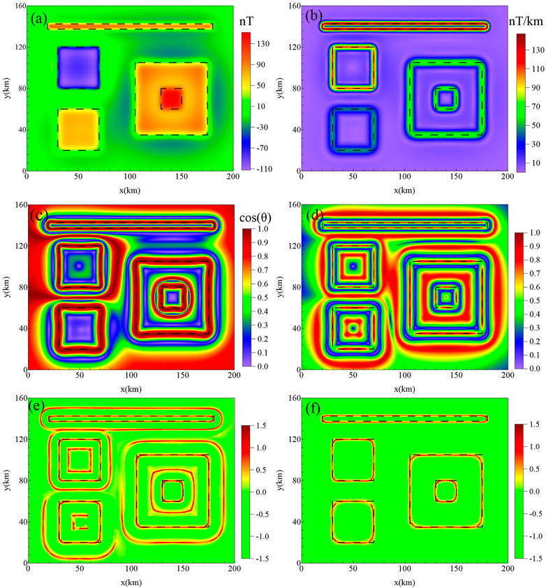
FIGURE 5. Example of the second synthetic model. (A) Synthetic magnetic anomaly caused by the five prisms; (B) HGA; (C) theta map; (D) NSTD; (E) SP-Gra; and (F) SP-Mag.

We also added random noise to the synthetic magnetic anomaly (Figure 5A) to estimate the effectiveness of the method in a noisy environment (Figure 6A). The random noise was introduced with an amplitude of 0.5% of the maximum data magnitude. The HGA (Figure 6B) and theta map (Figure 6C) filters can outline the edges of all sources, but the edges were blurred because of the effect of noise. Figure 6D shows the results of the NSTD method. We can see that the NSTD filter is less effective in outlining the edges of bodies M2, M3, and M4. Figure 6E shows the edges estimated by the SP-Gra method. In addition, the false edges affected by the noise become faintly visible. The edges estimated by SP-Mag are shown in Figure 6F. We can see that the SP-Mag provides a better outcome than the other filters, which can not only detect edges of all model bodies with high resolution but also show less sensitivity to noise and avoid bringing false edges in the map.

FIGURE 6

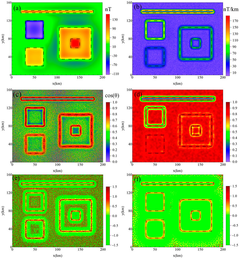
FIGURE 6. Synthetic magnetic anomaly of the second model corrupted by random noise with an amplitude equal to 0.5% of the maximum data magnitude, (A) synthetic magnetic anomaly caused by the five prisms; (B) HGA; (C) theta map; (D) NSTD; (E) SP-Gra; and (F) SP-Mag.

4 Application to field data

To test the performance of the SP-Mag method, it is applied together with the other four edge-enhancing methods to the RTP aeromagnetic anomaly of the Rizhao–Lianyungang area (indicated by the red rectangle in Figure 7). The magnetic field (Figure 8A) provides the high-accuracy aeromagnetic measurement with a grid cell size of 1 km × 1 km. The flight height of the data is 200 m, and the total measurement accuracy after leveling is ±1.35 nT. The aeromagnetic field is positive to the north and negative to the south on a whole and can be divided into two magnetic regions with Wenquan–Xufu–Rizhao as the boundary between them. The northern magnetic field is located in the large Jiaodong Peninsula with NE magnetic anomaly belts, which are characterized by strong magnetic anomaly intensity and local anomaly development. The eastern part of the southern magnetic region mainly corresponds to the Haizhouwan area, and the western part of this region is mainly covered by the Quaternary. In addition, the stratigraphy or magnetic rocks are only exposed in Donghai, Lianyungang, Guanyun, etc.

FIGURE 7

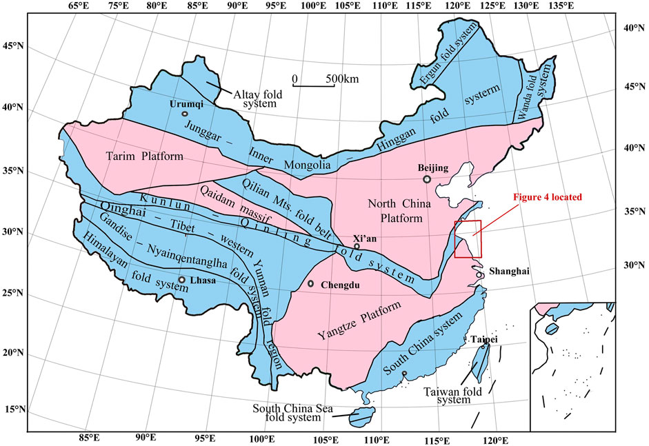
FIGURE 7. Geological sketch map of China (Sun et al., 2016a). The Rizhao–Lianyungang area in Figure 4 is indicated by the red rectangle. The pink color represents platform or massifs. The blue color represents tectonic or orogenic belts.

FIGURE 8

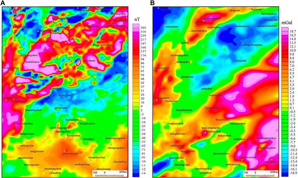
FIGURE 8. RTP aeromagnetic anomaly (A) and airborne gravity anomaly (B) of the Rizhao–Lianyungang area.

Edges outlined by the SP-Mag, HGA, theta map, NSTD, and SP-Gra methods from the RTP aeromagnetic anomaly of the Rizhao–Lianyungang area are shown in Figure 9. From Figure 9, one can obviously observe that regardless of the result detected by the SP-Gra method (Figure 9A) from the aeromagnetic anomaly or the results highlighted by the SP-Gra (Figure 9B), theta map (Figure 9D), and NSTD (Figure 9E) methods from the RTP aeromagnetic anomaly, all exhibit obvious false boundaries (e.g., areas declined by ellipse A). Compared with Figure 9A, the false edges detected by the SP-Gra (Figure 9B) from the RTP aeromagnetic anomaly were suppressed slightly (e.g., indicated by the arrow a), but they were still obvious. This is because the reduction to the pole can suppress the associated anomalies, but it cannot eliminate them. Figure 9C shows the result of the SP-Mag method. Compared with the other results, the SP-Mag significantly eliminates the false edges caused by the associated anomalies (e.g., area delineated by ellipse A in Figure 9C). The result of the SP-Mag method (Figure 9F) is more efficient for the later geological interpretation. For example, the boundary indicated by the rectangular box B in Figure 9C is the Lianyungang fault, which is difficult to be clearly identified in the other detected results because of the influence of false boundaries.

FIGURE 9

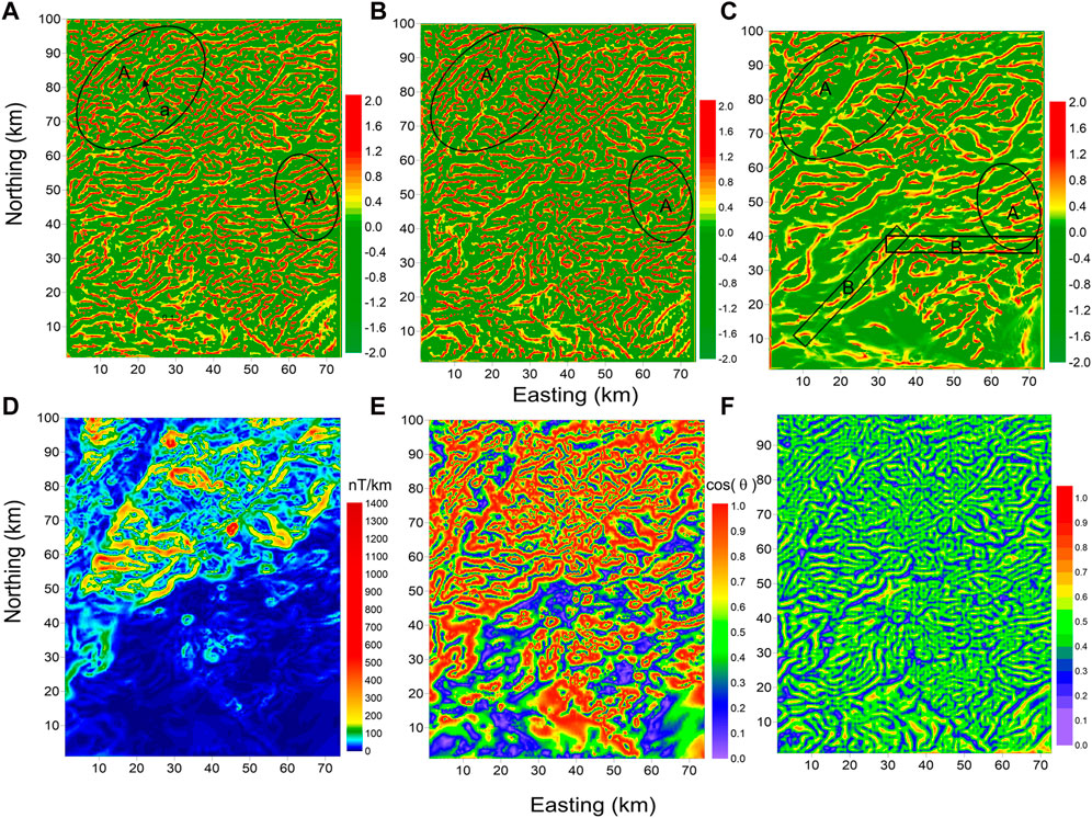
FIGURE 9. Test cases of edge-enhancing methods on the aeromagnetic anomaly of the Rizhao–Lianyungang area. The location has been outlined in the red rectangle in Figure 3. (A) SP-Gra from the aeromagnetic anomaly; (B) SP-Gra from the RTP aeromagnetic anomaly; (C) SP-Mag; (D) HGA from the RTP aeromagnetic anomaly; (E) theta map from the RTP aeromagnetic anomaly; and (F) NSTD from the RTP aeromagnetic anomaly.

In addition, SP-Mag can maintain the strong ability to enhance weak edges while eliminating the false boundary caused by the associated anomalies. For example, compared with the edges outlined by the HGA, the SP-Mag detects much edge information, especially in the southeast of the study area. In addition, edges detected by the SP-Mag are sharper than those detected from being covered by the strong boundaries. So the result of the SP-Mag can be more conducive to identify and track faults.

It is because the SP-Mag method eliminates the false boundary caused by the associated anomalies and the detected results can reflect the tectonic divisions more clearly. The result of the SP-Mag method (Figure 10A) is consistent with the tectonic division (Zhang et al., 2018) of the study area (Figure 11A). Figure 10A shows four obvious long and continuous belts A, B, C, and D that correspond to Yuli–Dadian, Wulian–Taoyuan, Donghai–Ganyu, and Sangxu–Lianyungang faults.

FIGURE 10

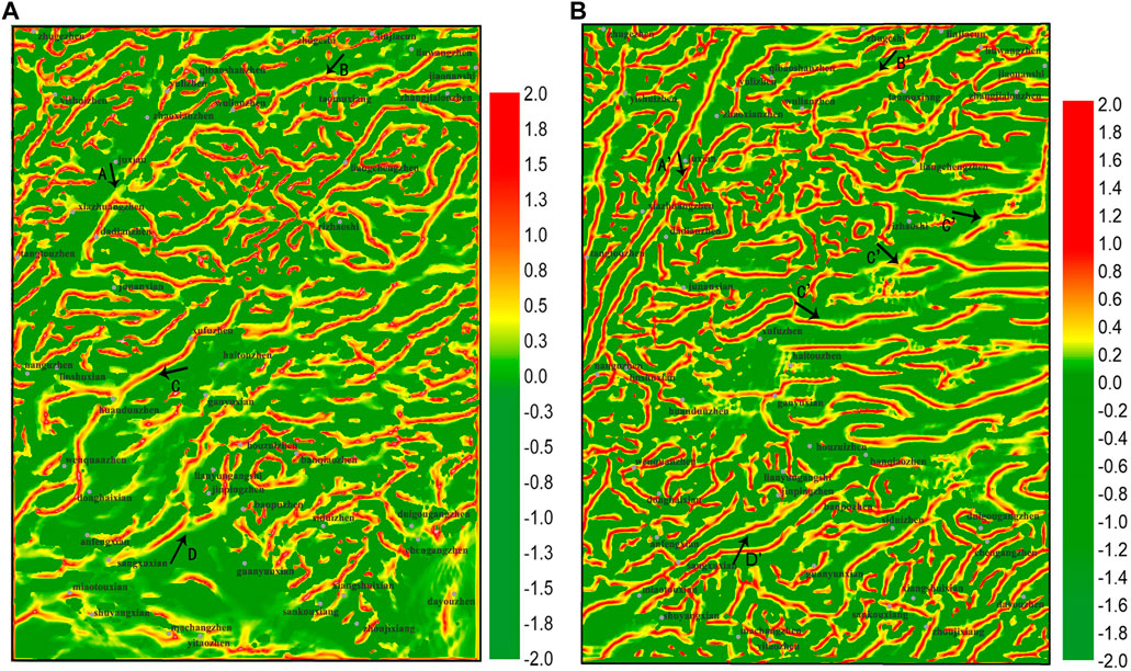
FIGURE 10. Edges detected from the aeromagnetic field (A) and airborne gravity field (B) by using the SP-Mag method.

FIGURE 11

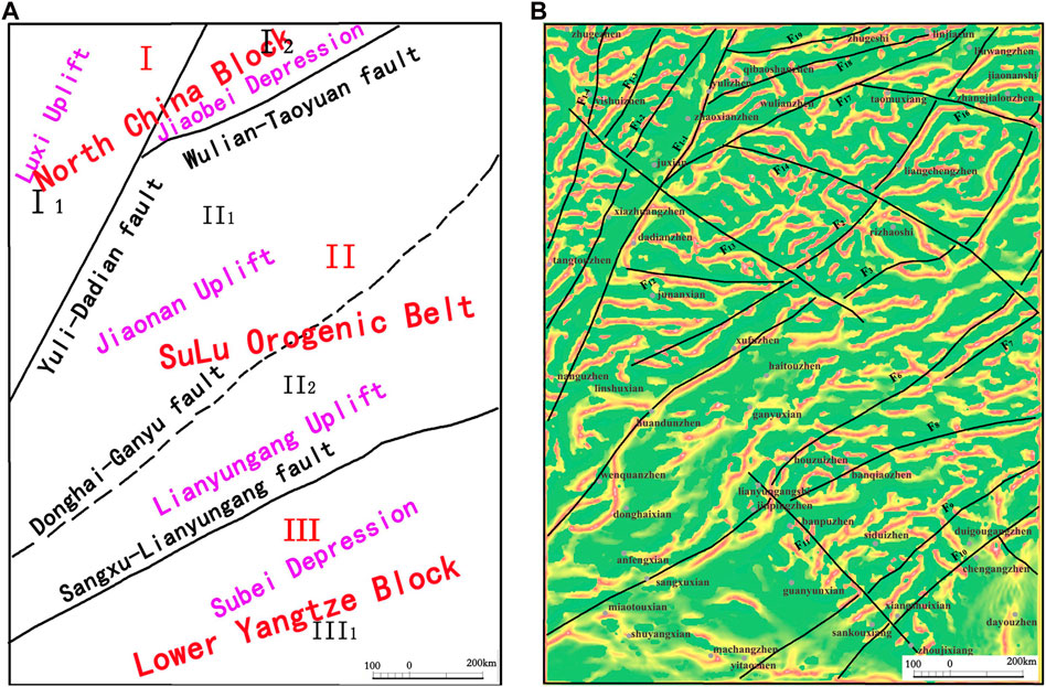
FIGURE 11. (A) Tectonic division sketch map; (B) map of the edges detected by using the SP-Mag method superimposed with the simplified geological map of the study region.

In order to learn the features of these faults, we also applied this method to the gravity field of the Rizhao–Lianyungang area. Figure 8B shows the airborne Bouguer gravity. The gravity field is measured with a grid cell size of 500 m × 500 m. The flight height of the data is 1,200 m, and the total measurement accuracy after leveling is ± 2.0×10⁻⁵ m/s². The gravity and magnetic anomalies in the study area have good homology. The Bouguer gravity field is high in the south and low in the north on a whole. The high-gravity anomalies spread to the NE direction and are mainly distributed in the Haizhouwan area and its southern land. The gravity anomalies in Qibaoshan and Xiazhuang–Nangu areas in the northwest of the study area are also relatively high, showing NNE-trending distribution, which are caused by the Precambrian basement uplift. The most obvious low-gravity anomaly is distributed in the Jiaonan area, which is mainly caused by the large area of Archaeo-Paleoproterozoic intermediate to acid rock mass.

The edge-enhanced results of the gravity field are shown in Figure 10B. It can be seen that the strikes of the detected edges are consistent with those of the magnetic field, reflecting the main structural strikes of NE and NNE in the study area. In addition, there are also obvious long and continuous belts A′, B′, and D′ corresponding to Yuli–Dadian, Wulian–Taoyuan, and Sangxu–Lianyungang faults. It is noteworthy that the Yuli–Dadian fault belongs to the Tanlu fault zone and is the eastern boundary of the Tanlu fault zone in the study area. Therefore, we can also find there are parallel lines on the left side of belt A′ in gravity edge-enhanced results. However, the belt C’ corresponding to the Donghai–Ganyu fault is no longer continuous anymore because the fault was staggered by late NW tectonic activities. It is well known that the magnetic field reflects magnetization information from the upper crust, while the gravity field can reflect density information from the whole crust. Yuli–Dadian, Wulian–Taoyuan, Donghai–Ganyu, and Sangxu–Lianyungang faults exist in the detected results from both magnetic and gravity fields, indicating they are all deep and large faults.

Furthermore, these four faults divided the study area into five structural regions and sub-regions (Figure 11A): west Shandong uplift zone (I₁), north Jiaodong uplift (I₂), south Jiaodong uplift (II₁), Lianyungang uplift (II₂), and north Jiangsu depression (III). The geometrical characteristics of the boundaries are obviously different in different structural partitions. Because of the control of the NNE Tanlu fault zone, boundaries in the west Shandong uplift zone are in the NE trends, while most boundaries in the south Jiaodong uplift zone are in the trends of EW direction. There develop several groups of NE parallel boundaries in north Jiangsu depression, and the boundaries in the Lianyungang uplift zone are disorderly, indicating crustal deformation is stronger here.

The edges detected by the SP-Mag method have also been compared with the fault structures. Figure 11B illustrates the edges recognized by the SP-Mag method, which is superimposed over a simplified geologic map (Zhang et al., 2018). The Rizhao–Lianyungang area has developed fault structures. In addition, the tectonic framework is composed of NE and NNE trending faults. The deep and large faults in the study area, which play an important role in controlling the regional structure, are the Tanlu fault zone (F1), Wulian–Taoyuan fault (F14), Sangxu–Lianyungang fault (F6), Rizhao–Liuwang fault (F2), Donghai–Ganyu fault (F5), and Yishui–Juxian fault (F13) (Zhang et al., 2018). Figure 11B displays that the edge coefficients show a good correlation with the geologic structures.

5 Discussion

It is well known that the short wavelength lineaments are mostly associated with shallower depth, whereas the longer wavelength lineaments are mostly related to the deep interior inside the Earth (Pham et al., 2020a). The HGA is dominated by the short wavelength lineaments (Figure 9D), and the SP-Gra, theta map, NSTD, and SP-Mag can delineate both the longer and smaller wavelengths’ structural and tectonic boundaries (Figures 9B, C, E, F). The SP-Gra, theta map, and NSTD maps indicate that the NE–SW and NW–SW trends are dominant in the data (Figures 9B, E, F). Although the SP-Gra, theta map, NSTD, and SP-Mag are effective in balancing lineaments associated with both shallow and deep depth, meanwhile the SP-Mag can eliminate false edges caused by the associated anomalies. In the practical application, a large amount of false edges and some small-scale partial boundaries are eliminated; thus, the detected edges are more suitable to highlight the whole structure pattern and trace the faults. Figure 12 shows the lineaments detected by the SP-Mag map. In addition, the trend analysis of the mapped lineaments has been statistically computed in the form of the rose diagram (Figure 13). The diagram shows the dominant lineament trends in NE–SW and NW–SW orientations, which is in accordance with the fault trends shown in Figure 6. The obtained results illustrate the usefulness of the SP-Mag for potential field interpretation.

FIGURE 12

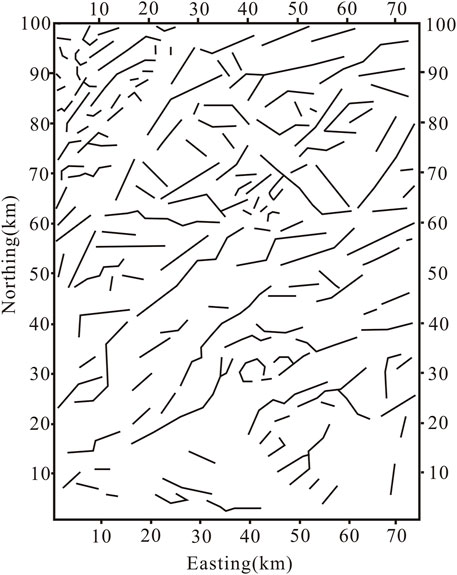
FIGURE 12. Lineaments detected from the SP-Mag map of the magnetic data.

FIGURE 13

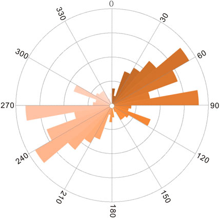
FIGURE 13. Rose diagram of the lineaments in Figure 12.

The proposed method uses the idea of the pseudo-gravity field, but there is no need for the calculation of the pseudo-gravity field. Instead, we calculate two horizontal components of magnetic anomaly—Hax and Hay—and hence avoid losing details caused by the local truncation errors. In addition, when the associated anomalies are not very serious in the magnetic field in the study area, we can use the SP-Gra method directly to outline the edges; when the regional magnetic field is with serious associated anomalies, one can select the SP-Mag method to detect these edges. Although the SP-Mag can recognize lineaments effectively, more geological and geophysical data should be still combined for comprehensive interpretation in the actual interpretation.

Furthermore, we have conducted some three-component aeromagnetic surveys, obtaining data Hax, Hay, and Za. Therefore, the SP-Mag method can directly use the two horizontal components Hax and Hay to enhance the edges. Furthermore, this work will be carried out in the following study.

6 Conclusion

We have proposed a modified magnetic edge-detection method (SP-Mag) based on the second-order spectral moment. This method has been demonstrated using both synthetic and field data. The synthetic test shows that SP-Mag can not only balance edges regardless of strong or weak anomalies but also eliminate those false edges caused by the associated anomalies in the magnetic field, which provides more effective information for subsequent interpretation. Using the RTP aeromagnetic field of the Rizhao–Lianyungang area as an example, the detected results can provide clearer details, and the lineaments detected by the SP-Mag method are consistent with geological structures.

Data availability statement

The data analyzed in this study are subjected to the following licenses/restrictions: the original aeromagnetic data are unavailable. The analyzed data are available from the authors upon reasonable request and by permission of China Aero Geophysical Survey and Remote Sensing Center for Natural Resources. Requests to access these datasets should be directed to Sun Yanyun, yysun2009@126.com.

Author contributions

YS conceived the idea and made overarching research goals and aims and wrote the manuscript. XZe contributed to the conception of the study and helped to deduce the formula. WY contributed to analysis and manuscript preparation, critical review, and commentary or revision—including pre- or post-publication stages. XL contributed to data processing through software and codes. WZ contributed to the geological interpretations of the edge results extracted from the aeromagnetic data. XZh contributed to the analysis with constructive discussions. All authors approved the final draft of the manuscript.

Funding

The authors gratefully acknowledge the financial support from the National Science Foundation of China (Grant No. 42104138) and the Geological Survey Project (No. DD20221715, No. DD20230069).

Conflict of interest

The authors declare that the research was conducted in the absence of any commercial or financial relationships that could be construed as a potential conflict of interest.

Publisher’s note

All claims expressed in this article are solely those of the authors and do not necessarily represent those of their affiliated organizations, or those of the publisher, the editors, and the reviewers. Any product that may be evaluated in this article, or claim that may be made by its manufacturer, is not guaranteed or endorsed by the publisher.

References

Blakely, R. J., and Simpson, R. W. (1986). Approximating edges of source bodies from magnetic or gravity anomalies. Geophysics 51, 1494–1498. doi:10.1190/1.1442197

CrossRef Full Text | Google Scholar

Cooper, G. R. J. (2009). Balancing images of potential field data. Geophysics 74 (3), 17–20. doi:10.1190/1.3096615

CrossRef Full Text | Google Scholar

Cooper, G. R. J., and Cowan, D. R. (2011). A generalized derivative operator for potential field data. Geophys. Prospect. 59, 188–194. doi:10.1111/j.1365-2478.2010.00901.x

CrossRef Full Text | Google Scholar

Cooper, G. R. J., and Cowan, D. R. (2008). Edge enhancement of potential-field data using normalized statistics. Geophysics 73 (3), 1–4. doi:10.1190/1.2837309

CrossRef Full Text | Google Scholar

Cordell, L. (1979). “Gravimetric expression of graben faulting in santa Fe country and the espanola basin,” in 30th field conference (New Mexico: Geological Society Guidebook), 59–64.

CrossRef Full Text | Google Scholar

Eldosouky, A. M., Pham, L. T., and Henaish, A. (2022). High precision structural mapping using edge filters of potential field and remote sensing data: A case study from wadi umm ghalqa area, south eastern desert, Egypt. Egypt J. Remote Sens. Space Sci. 25 (2), 501–513. doi:10.1016/j.ejrs.2022.03.001

CrossRef Full Text | Google Scholar

Evjen, H. M. (1936). The place of the vertical gradient in gravity interpretation. Geophysics 1, 127–136. doi:10.1190/1.1437067

CrossRef Full Text | Google Scholar

Fedi, M., and Florio, G. (2001). Detection of potential fields source boundaries by enhanced horizontal derivative method: Potential field sources boundaries by EHD method. Geophys. Prospect. 49, 40–58. doi:10.1046/j.1365-2478.2001.00235.x

CrossRef Full Text | Google Scholar

Francisco, F. J., de Souza, A., Bongiolo, A. B. S., and Castro, L. G. (2013). Enhancement of the total horizontal gradient of magnetic anomalies using the tilt angle. Geophysics 78 (3), J33–J41. doi:10.1190/GEO2011-0441.1

CrossRef Full Text | Google Scholar

Guan, Z. L. (2005). Geomagnetic field and magnetic exploration. Beijing: Geological Publishing House Press.

Google Scholar

Guan, Z. L., and Yao, C. L. (1997). Inversion of the total gra dient modulus of magnetic anomaly due to dipping dike (in Chinese). Earth Sci. J. China Uni. Geosci. 22 (1), 81–85.

Google Scholar

Hansen, R. O., and de Ridder, E. (2006). Linear feature analysis for aeromagnetic data. Geophysics 71 (6), L61–L67. doi:10.1190/1.2357831

CrossRef Full Text | Google Scholar

Hu, S. G., Tang, J. T., and Ren, Z. Y. (2019). Normalized facet edge detection and enhancement in potential field sources with the scale-space technique. Chin. J. Geophys. 62 (1), 331–342. doi:10.6038/cjg2019L0317

CrossRef Full Text | Google Scholar

Huang, Y. Y. (1985). Geometrical interpretation and graphical solution of second order spectrum moments and statistical invariants for random surface characterization. J. Zhejiang Univ. 6 (19), 143–153.

Google Scholar

Hu, Z. G., Yu, Q. F., and Lou, H. (1995). 3-D analytic signal method (in Chinese). Computing techniques for geophysical and geochemical exploration 17 (3), 36–42.

Google Scholar

Li, C. G., Dong, S., and Zhang, G. X. (2000). Evaluation of the anisotropy of machined 3D surface topography. Wear 237, 211–216. doi:10.1016/S0043-1648(99)00327-0

CrossRef Full Text | Google Scholar

Ma, G. Q., Huang, D. N., Yu, P., and Li, L. L. (2012). Application of improved balancing filters to edge identification of potential field data (in Chinese). Chin. J. Geophys. 55 (12), 4288–4295. doi:10.6038/j.issn.0001-5733.2012.12.040

CrossRef Full Text | Google Scholar

Miller, H. G., and Singh, V. (1994). Potential field tilt - a new concept for location of potential field sources. J. Appl. Geophys. 32, 213–217. doi:10.1016/0926-9851(94)90022-1

CrossRef Full Text | Google Scholar

Nabighian, M. N. (1972). The analytic signal of two-dimensional magnetic bodies with polygonal cross-section: Its properties and use for automated anomaly interpretation. Geophysics 37, 507–517. doi:10.1190/1.1440276

CrossRef Full Text | Google Scholar

Pham, L. T., Eldosouky, A. M., Melouah, O., Abdelrahman, K., Alzahrani, H., Oliveira, S. P., et al. (2021). Mapping subsurface structural lineaments using the edge filters of gravity data. J. King Saud. Univ. Sci. 33 (8), 101594. doi:10.1016/j.jksus.2021.101594

CrossRef Full Text | Google Scholar

Pham, L. T., Eldosouky, A. M., Oksum, E., and Saada, S. A. (2020a). A new high resolution filter for source edge detection of potential field data. Geocarto Int. 37, 3051–3068. doi:10.1080/10106049.2020.1849414

CrossRef Full Text | Google Scholar

Pham, L. T., Van Vu, T., Le Thi, S., and Trinh, P. T. (2020b). Enhancement of potential fieldsource boundaries using an improved logistic filter. Pure Appl. Geophys 177 (11), 5237–5249. doi:10.1007/s00024-020-02542-9

CrossRef Full Text | Google Scholar

Phillips, J. D., Hansen, R. O., and Blakely, R. J. (2007). The use of curvature in potential-field interpretation. Explor. Geophys. 38, 111–119. doi:10.1071/EG07014

CrossRef Full Text | Google Scholar

Prasad, K. N. D., Pham, L. T., Singh, A. P ., Eldosouky, A. M., Abdelrahman, K., Fnais, M. S., et al. (2022). A novel EnhancedTotal gradient (ETG) forInterpretation of magnetic data. Minerals 12, 1468. doi:10.3390/min12111468

CrossRef Full Text | Google Scholar

Roest, W. R., Verhoef, J., and Pilkington, M. (1992). Magnetic interpretation using the 3-D analytic signal. Geophys. 57, 116–125. doi:10.1190/1.1443174

CrossRef Full Text | Google Scholar

Sun, Y. Y., Yang, W. C., Zeng, X. Z., and Zhang, Z. Y. (2016a). Edge enhancement of potential field data using spectral moments. Geophysics 81, G1–G11. doi:10.1190/geo2014-0430.1

CrossRef Full Text | Google Scholar

Sun, Y. Y., Yang, W. C., and Yu, C. Q. (2016b). Multi-scale scratch analysis in Qinghai-Tibet plateau and its geological implications. Pure Appl. Geophys. 173, 1197–1210. doi:10.1007/s00024-015-1153-3

CrossRef Full Text | Google Scholar

Sun, Y. Y., Yang, W. C., Zeng, X. Z., Zhao, T. Y., Zhang, W., Zhang, X. J., et al. (2022). Scratch recognition and analysis of gravity field in Chinese continent. Acta Geophys. 70, 2001–2012. doi:10.1007/s11600-022-00899-0

CrossRef Full Text | Google Scholar

Thomas, T. R. (1982). Rough surfaces. London: Longman Group UK Limited.

Google Scholar

Verduzco, B., Fairhead, J. D., Green, C. M., and MacKenzie, C. (2004). New insights into magnetic derivatives for structural mapping. Lead. Edge 23, 116–119. doi:10.1190/1.1651454

CrossRef Full Text | Google Scholar

Wang, Y. G., Zhang, F. X., Wang, Z. W., Meng, L. S., and Zhang, J. (2013). Edge detection of potential field using normalized differential (in Chinese). J. Jilin Univ. (Earth Sci. Ed. 43 (2), 591–602.

Google Scholar

Wijins, C., Perez, C., and Kowalczyk, P. (2005). Thetamap: Edge detection in magnetic data. Geophysics 70 (4), L39–L43. doi:10.1190/1.1988184

CrossRef Full Text | Google Scholar

Yang, S. Z., Wu, Y., and Xuan, J. P. (1992). Time series analysis in engineering and application. Wuhan: Huazhong University of Science and Technology Press.

Google Scholar

Yang, W. C., and Sun, Y. Y. (2016). Discovering crustal deformation bands by processing regional gravity field. Acta Geol. Sin. Engl. Ed. 90 (2), 66–74. doi:10.1111/1755-6724.12642

CrossRef Full Text | Google Scholar

Yang, W. C., Sun, Y. Y., Hou, Z. Z., and Yu, C. Q. (2015). A multi scale scratch analysis method for quantitative interpretation of regional gravity fields. Chin. J. Geophys. 58, 41–53. doi:10.1002/cjg2.20154

CrossRef Full Text | Google Scholar

Yang, W. C., Sun, Y. Y., Hou, Z. Z., and Yu, C. Q. (2017). A study on spectral moments of gravity field with application to crustal structure imaging of Tarim basin (in Chinese). Chin. J. Geophys. 60(8), 3140–3150. doi:10.6038/cjg20170821

CrossRef Full Text | Google Scholar

Zeng, X. Z., Sun, Y. Y., Yu, C. Q., and Liu, S. B. (2018). Edge enhancement of magnetic field based on spectral moments and pseudo-gravity field. California, CA: Soc Exploration Geophysicists, 1494–1498.

Google Scholar

Zhang, H. L., Dhananjay, R., Marangoni, Y. R., and Hu, X. Y. (2014). NAV- Edge: Edge detection of potential-field sources using normalized anisotropy variance. Geophysics 79 (3), J43–J53. doi:10.1190/geo2013-0218.1

CrossRef Full Text | Google Scholar

Zhang, W., Zhang, X. J., Tong, J., and Fan, Z. (2018). Gravity and magnetic anomaly characteristics and its geological interpretation in rizhao-lianyungang areas. Earth-Science 43 (12), 4490–4497. doi:10.3799/dqkx.2018.518

CrossRef Full Text | Google Scholar