A multi-target prediction model for dam seepage field

Prediction of dam behavior based on monitoring data is important for dam safety and emergency management. It is crucial to analyze and predict the seepage field. Different from the mechanism-based physical models, machine learning models predict directly from data with high accuracy. However, current prediction models are generally based on environmental variables and single measurement point time series. Sometimes point-by-point modeling is used to obtain multi-point prediction values. In order to improve the prediction accuracy and efficiency of the seepage field, a novel multi-target prediction model (MPM) is proposed in which two deep learning methods are integrated into one frame. The MPM model can capture causal temporal features between environmental variables and target values, as well as latent correlation features between different measurement points at each moment. The features of these two parts are put into fully connected layers to establish the mapping relationship between the comprehensive feature vector and the multi-target outputs. Finally, the model is trained for prediction in the framework of a feed-forward neural network using standard back propagation. The MPM model can not only describe the variation pattern of measurement values with the change of load and time, but also reflect the spatial distribution relationship of measurement values. The effectiveness and accuracy of the MPM model are verified by two cases. The proposed MPM model is commonly applicable in prediction of other types of physical fields in dam safety besides the seepage field.

1 Introduction

A dam is a complex and important water retaining structure in the field of hydraulic engineering. Because the dam possesses huge amounts of hydraulic energy, once it is broken, the flood will cause immeasurable damage to the lives and properties of people downstream. It is of great practical importance to know the operational behavior of the dam and predict its development through dam safety monitoring (Wu and Su, 2005; Jeon et al., 2009; Gu et al., 2016).

Two types of methods can be used to establish dam behavior prediction models: physics-driven methods and data-driven methods. Physics-driven methods mainly use finite element method to predict and analyze the physical field of the dam according to the constitutive model based on the physical and mechanical relationships of materials (Gu et al., 2011; Huang and Chen, 2012). The physics-driven methods essentially reveal the operational behavior of the main physical fields of the dam. However, these approaches place high demands on constitutive models, which limits the applicability of such approaches. Data-driven methods, which are based on regression analysis of historical monitoring data and influencing factors can be subdivided into two categories: One is the traditional statistical model (Fanelli, 1975; Bonelli and Royet, 2001; Deng et al., 2007), which is the most frequently used data-driven method in practical engineering applications due to its definite physical meaning and simple application. The statistical model physically explains and predicts dam behavior rules. However, this model needs to establish a functional relationship between effect variables (dependent variables) and influencing factors (independent variables) (Zhu et al., 2019; Liang et al., 2022; Tang et al., 2022) based on mathematical statistics theory. The selection of appropriate independent variables is difficult to determine because the operational behavior of the dam is affected by many complex factors and the influence of different factors on the behavior of the dam is unstable. All these factors lead to low prediction accuracy of the statistical model. The other is the most advanced machine learning method (Su et al., 2000). A more typical method is to use neural networks to establish complex non-linear and time-varying input-output relationships between effect variables and influencing factors. For example, Su et al. (2001) used the fuzzy neural network to establish the functional relationship between the horizontal displacement of the dam crest and water level, temperature, and time effect. Shi et al. (2020) used the radial basis function neural network optimized by the genetic algorithm to predict the seepage discharge of the concrete face rockfill dam. Hou et al. (2022) combined time series decomposition and deep learning to predict the deformation of high embankment dams. Azarafza et al. (2021), Azarafza et al. (2022), and Nikoobakht et al. (2022) have also done much research work based on deep learning to verify its advantages in landslide susceptibility assessment, landslide susceptibility mapping, and prediction of geotechnical features of rock materials. To give a brief summary, Table 1 is presented to describe about deep learning models, along with the application in dam behavior prediction, as well as their advantages and disadvantages. More information can be found in the literatures (Xu et al., 2019; Ren et al., 2021). From these studies, we can conclude that neural networks have a high potential for dam behavior prediction. However, due to the large amount of noise interference in the monitoring data, the prediction accuracy of the model is likely to be low due to overfitting. Moreover, the above data-driven methods are all for the prediction of single measurement point, which cannot well predict the main physical fields of dam behavior with multiple measurement points.

TABLE 1

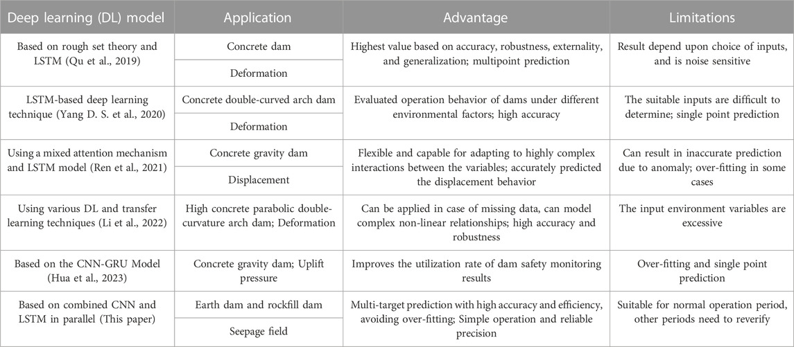
TABLE 1. A summary of deep learning in dam behavior prediction.

The single measurement point prediction model plays an important role in explaining the operation rules of the dam and implementing safety monitoring, but it does not involve the interconnection between multiple measurement points. It only reflects the structural state of the location of single measurement point, which has limitations. Even if multiple single measurement point prediction models are used to obtain predictions of multiple measurement points, the rules described by them are often not consistent and coordinated. Multiple target learning (MTL) (Caruana, 1993) is a modeling method that accounts for latent correlation between target values at multiple measurement points by sharing parameters and simultaneously predicts multiple target values in the physical field by training a model. Training multiple targets in parallel is equivalent to implicitly increasing the amount of training data, which reduces the risk of overfitting and improves the prediction accuracy and efficiency. The main parameter of sharing patterns in MTL models include hard parameter sharing (Caruana, 1993) and soft parameter sharing (Misra et al., 2016; Gao et al., 2019). Hard parameter sharing means that multiple target-specific output layers are maintained and all target values are forced to use the same parameters to obtain a common parameter model. Soft parameter sharing is simpler and more flexible than hard parameter sharing because each target is assigned its own set of parameters and the parameters are partially shared through some mechanism. The main difficulty in developing MTL models is the need to exploit correlations and differences between targets. The initial applications of MTL models for dam behavior prediction include: Yao et al. (2022) performed an improved multi-output support vector machine, and the improved model considered chaos and similarity of displacement series to simultaneously predict displacements of multiple measurement points with the same trend. Chen et al. (2022) proposed a serial model composed of convolutional neural networks and convolutional long short-term memory networks to extract spatial features from multiple measurement values and temporal features in time series in turn, and then simultaneously predict displacements of multiple measurement points. This method focused on statistical rules for target series without environmental variables.

In summary, there is a wealth of theoretical research results for dam behavior prediction models, but less research on the seepage field prediction based on deep learning. Seepage failure is one of the major causes of dam failure (Foster et al., 2000). The analysis and prediction of the seepage field has important implications for dam safety (Deng et al., 2020). The objective of this study is to establish an efficient and accurate the seepage field prediction model for the simultaneous prediction of seepage at multiple measurement points. It is well known that the response of dam seepage field to changes in environmental variables is non-synchronous, and the rules for the temporal development of target values at different measurement points are related to the location of the measurement points. The longer the period and the smaller the variation of target values of points closer to the downstream, while those closer to the upstream are not (i.e., the variation trend of target values at different measurement points is similar but not the same at any one time). When multi-target prediction is performed and hard parameter sharing is applied, it forces the regularity of each measurement point at any time to be consistent, affecting prediction accuracy. Applying soft parameter sharing to learn the differences between target values can effectively improve the learning capacity of the model. Given its strong ability to capture local features for adjacent target values (Krizhevsky et al., 2012), the convolutional neural networks (CNN) model is introduced as the soft parameter sharing layer. Since the temporal variation trends of target values at different measurement points are highly similar and both target values and environmental variables have strong time series characteristics, the long short-term memory networks (LSTM) model, which is superior in processing sequential data, is introduced to extract causal temporal features between environmental variables and target values. For dam seepage prediction, no evidence has been found at present for using a combination of CNN and LSTM in parallel. Therefore, based on the causal relationship between external loads and seepage field distribution, this study combines CNN and LSTM in parallel to establish a novel multi-target prediction model (MPM) for simultaneous predictions at multiple measurement points. The MPM model can not only describe the variation regulation of measurement values with the change of load and time, but also reflect the spatial distribution relationship of measurement values by considering the correlation information among multiple measurement points, which is undoubtedly more comprehensive and real for correctly mastering the structural condition and variation rules of the whole dam. The MPM model improves prediction accuracy and efficiency while also achieving seepage field prediction. It is of great importance to effectively and safely manage reservoir operation, as well as to improve future planning for dam seepage problems.

2 The novel prediction model

2.1 The existing models adopted

2.1.1 Long-short term memory model

Long short-term memory networks (LSTM) (Hochreiter and Schmidhuber, 1997) are an extension of recurrent neural network designed to solve the problem of long-term dependencies and vanishing gradients. In LSTM, it can continuously learn short-term time changes and long-periodic variation rules (Hochreiter, 1998) due to its connection to hidden nodes. LSTM has a stronger temporal feature extraction capability and a faster training speed for time series (Zhao et al., 2021). Because of these characteristics, LSTM produced good performance in predicting dam behavior series (Zhao et al., 2021; Hou et al., 2022). LSTM is also one of the most widely adopted models for MTL models (Wan et al., 2021; Zong et al., 2022). For non-linear regression, LSTM can be used to obtain highly-accurate predictions, and its governing equation can be simplified as follows:

$h_t,c_t=LSTM\left(x_t,h_{t-1},c_{t-1}\right)(1)$

where x_t is the input vector, c is the memory cell, and h is the hidden layer.

The LSTM model in this paper contains multiple hidden layers (Luo et al., 2022) to extract deep causal temporal features. The output of the last hidden layer of LSTM is recorded as $F_t^{d_1}$ after flattening so as to facilitate feature fusion and connect fully connected layers.

2.1.2 Convolutional neural networks

Convolutional neural networks (CNN) (Hubel and Wiesel, 1959; LeCun and Bengio, 1995) are mainly used to process variables in Euclidean space (Hakim et al., 2021). The convolutional layer, the pooling layer, and the activation function of the CNN model are the core steps of feature extraction. The convolutional layers extract the different non-linear interaction relationship features of the input data by setting different convolution kernels. The pooling layer reduces redundant features by taking the maximum or average value of the data in the convolution kernel. The activation function reflects the mapping relationship between input and output in two adjacent layers, which provides neural networks with non-linearity capability.

In this paper, the CNN model is introduced to extract latent features between adjacent target values. The input is a data grid with multiple measurement values at each moment that is regularly arranged, and high-dimensional feature extraction is performed using a series of convolutions and maximum pooling subsampling. The activation function is the rectified linear unit (Relu). Finally, it is flattened into a one-dimensional feature vector $F_s^{d_2}$ to facilitate feature fusion and to connect fully connected layers.

2.2 The framework of the MPM model

The seepage field contains multiple measurement points that can be meshed at each moment to produce a series of data grids (Figure 1A). The position of the measurement points is indexed by coordinates, and there is at most one measurement value in each small square, and no measurement value is assigned 0. The data grid at each moment is similar to the images that CNN usually processes. The measurement value of each point in the data grid is typical time series data, which is suitable for analysis by LSTM. Similar trends and differences can be seen among time series (Figures 1B, C).

FIGURE 1

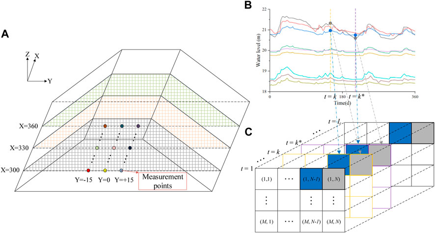
FIGURE 1. Similar trends and differences of target values. (A) Mesh. (B) Time series. (C) Data grids.

The MPM model consists of two different parallel networks, CNN and LSTM (the framework is shown in Figure 2). The LSTM model efficiently captures causal temporal features. By constructing a data grid with multiple target values at each moment, the CNN model with local feature extraction capability adaptively deep mines latent features from the data grid to optimize the multi-target model. Latent correlation features between target values learned by CNN are fused with causal temporal features extracted by LSTM, and the final multi-target predictions are obtained by fully connected layer mapping.

FIGURE 2

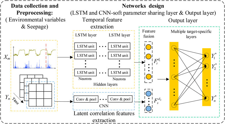
FIGURE 2. The framework of the MPM model.

For specific data processing, preprocessed environmental variables and monitoring history data are fed into the MPM model, the temporal features are extracted by the LSTM model, correlation features between target values are extracted by the CNN-soft parameter sharing layer, flattened feature vectors are obtained for feature fusion at the same time, and the respective outputs of multiple target values are connected by fully connected layers. The MPM model integrates CNN and LSTM into a unified framework for jointly training one loss function. In addition, since the MPM model has multiple outputs, back propagation is carried out in parallel. A standard back propagation algorithm propagates errors from the output layer to the feature fusion layer and then to the parallel network layer and updates parameters.

The parts are described below:

(1) Data collection and preprocessing: abnormal data were eliminated, and data format conventions and normalization were carried out for environmental variables and target values (Yang D. S. et al., 2020) to make them suitable for the MPM model. Inputs are X_m and Y_n, where X is a matrix of m environmental variables and Y is a matrix of n target values.

(2) Soft parameter sharing layer: Soft parameter sharing layer is built by CNN with local perception and weight sharing features. The CNN model is introduced to mine latent correlation features between target values of adjacent measurement points.

(3) Feature fusion layer: There are two main feature fusion methods in hybrid neural networks: addition (Yang J et al., 2020) and concatenation (Zhang et al., 2022). Feature addition requires the same dimension of feature vectors, while concatenation is more flexible. Moreover, feature fusion through concatenation has the effect of reinforcing and interconnecting features (Zhang et al., 2017; Zhang et al., 2022). Therefore, concatenation is used to fuse feature vectors in MPM.

(4) Output layer: Fully connected layers are performed to connect the final multi-target outputs, which consist of an input layer, hidden layers, and an output layer. The input to this module is the comprehensive feature vector. Full connection between adjacent layers is used to integrate local information, and the corresponding activation function is set to achieve non-linearity. Due to data regression, the activation function is sigmoid. For neural networks, when the input data is not very large, the 2- to 3-layer structure can fit any function (Yan et al., 2019).

2.3 The detailed calculation method

2.3.1 Model training

Details of the MPM model are presented in Algorithm 1.

Algorithm 1:. The MPM model.

Input: Environmental variables X_m and target values Y_n

1. Data preprocessing

2. Get training and test datasets

3. Randomly initialize model parameters

4. Set loss function: RMSE

5. Begin training:

6.  Forward propagation

7.  Calculate loss function

8.  Calculate gradient descent

9.  Backpropagation and update model parameters

10. End training

11. Save model parameters

12. Begin testing

13. Inverse standardization

Output: The predictions of ${\mathit{Y}}_{\mathit{n}}^{*}$

The specific training process is as follows (Figure 3):

FIGURE 3

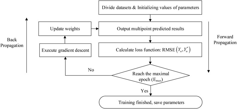
FIGURE 3. Flow chart of the MPM training process.

Step 1:. Obtain the initial training dataset and initialize the model parameters.

Step 2:. Enter the training data into the networks to start the training. According to the output predictions and target values, the error of multiple measurement points on the output layer is calculated and then propagated forward to the feature fusion layer and the parallel layer, where the error is calculated.

Step 3:. Update the weights according to the error on the output layer and calculate the total error of the multi-target results. If the maximum number of iterations is reached, proceed directly to Step 4. Otherwise, Step 2 is returned.

Step 4:. Model training is completed, and the configuration of the entire network is saved for prediction.

2.3.2 Hyperparameter optimization

The goal of hyperparameter optimization is to make the model perform better on both training and test datasets. At present, there is no perfect theoretical guidance for the selection of hyperparameters of deep neural networks, which need to be constantly adjusted according to the learning effect of the model. In order to obtain the optimal structure of the deep learning model, this study adopts the variable control approach to select hyperparameters such as the number of network layers, the number of neurons, and the number of iterations, taking into account the prediction accuracy and complexity of the model.

2.4 Comparison model and evaluation metrics

To verify the effectiveness of the MPM model, it is compared and analyzed with the traditional multi-target benchmark model based on hard parameter sharing (Zhou et al., 2018; Sun et al., 2021). For convenience, the benchmark model is denoted LSTM-M in this paper. Hard parameter sharing layer of the LSTM-M model is built by LSTM neural networks, and the output results are target-specific and built by fully connected layers. The LSTM-M model based on hard parameter sharing can share complementary knowledge between various time series and capture temporal features between environmental variables and target values. For fair comparison, the hyperparameters and inputs of the LSTM-M model are consistent with those of the MPM model.

In order to examine the superiority of the MPM model from different perspectives, mean square error (MSE), root mean square error (RMSE), mean absolute error (MAE), coefficient of determination (R²), and mean absolute percentage error (MAPE) are five commonly used metrics to fully compare and evaluate predictive performance. Among them, R² reflects fit performance, ranging from 0 to 1, and a more significant R² represents a better fit. MSE and RMSE are sensitive to outliers and can measure deviations between predictions and target values. MAE is the mean of the absolute value of the error, and MAPE measures the absolute difference between predictions and target values, with a smaller value representing better prediction performance. The equations are as follows:

$MSE=\frac{1}{M\cdot N}{\displaystyle \sum _{j=1}^M}{\displaystyle \sum _{i=1}^N}{\left({\widehat{y}}_{j,i}-y_{j,i}\right)}^2(2)$

$RMSE=\frac{1}{M}{\displaystyle \sum _{i=1}^M}\sqrt{\frac{1}{N}{\displaystyle \sum _{j=1}^N}{\left({\widehat{y}}_{j,i}-y_{j,i}\right)}^2}(3)$

$MAE=\frac{1}{M}{\displaystyle \sum _{i=1}^M}\left(\frac{1}{N}{\displaystyle \sum _{j=1}^N}\left|{\widehat{y}}_{j,i}-y_{j,i}\right|\right)(4)$

$R^2=\frac{1}{M}{\displaystyle \sum _{i=1}^M}\left(1-\frac{{\displaystyle \sum _{j=1}^N}{\left({\widehat{y}}_{j,i}-y_{j,i}\right)}^2}{{\displaystyle \sum _{j=1}^N}{\left(y_{j,i}-{\overline{y}}_{j,i}\right)}^2}\right)(5)$

$MAPE=\frac{100\%}{M\cdot N}{\displaystyle \sum _{i=1}^M}{\displaystyle \sum _{j=1}^N}\left|\frac{{\widehat{y}}_{j,i}-y_{j,i}}{y_{j,i}}\right|(6)$

where $\widehat{y}$ is the predicted value, $y$ is the measurement value, ${\overline{y}}_i$ is the mean value of target values, N is the number of samples, and M is the number of measurement points.

In addition, to directly analyze the prediction performance of two models, the promotion percentages of MSE, RMSE, MAE, and MAPE are applied. The index can be expressed as Eq. 7, where EM represents different evaluation metrics and the positive value represents that the second model has better performance than the first. The higher the ratio, the greater the performance improvement of the model.

$P=\frac{E{M}_1-E{M}_2}{E{M}_1}\cdot 100\%(7)$

3 Applications and result analysis

3.1 The first model application

3.1.1 Project status and monitoring data profile

Naban (Sun, 2012) is an earth dam with a clay core wall, a crest elevation of 231.5 m, a maximum height of 78.5 m, a crest width of 8.0 m, a normal reservoir water level of 220.2 m, and a dead water level of 209.6 m. Reservoir water level (RWL) and rainfall are environmental variables. Given the low downstream water level and little fluctuation, the influence of the downstream water level is not considered in this case. The total water head measured by six piezometer tubes in the maximum height section is selected as the representative measurement value, denoted R1–R6. The position of multiple piezometer tubes is shown in Figure 4.

FIGURE 4

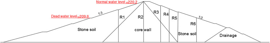
FIGURE 4. Piezometric tubes distribution of the Naban earth dam.

3.1.2 Training and prediction

There were 969 observations from 24 May 2001, to 31 December 2010. The time series of monitoring data is shown in Figure 5.

FIGURE 5

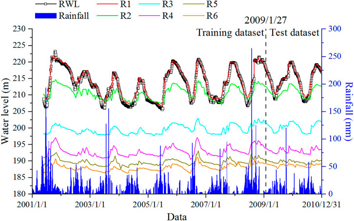
FIGURE 5. Time series of monitoring data.

The dataset from 24 May 2001 to 27 January 2009, is used as training data for optimizing and adjusting parameters, and the dataset from 30 January 2009 to 31 December 2010, is used as test data for prediction and performance evaluation.

In this case, the CNN model has two convolutional layers with 8 neurons and 2 and 3 convolution kernels, respectively. The LSTM model has 16 neurons in the two hidden layers, and the fully connected layers have two hidden layers. The batch size is 64, the number of iterations (epoch) is set to 1,000, Adam is the optimizer, the initial learning rate is set to 0.001, and the dropout rate is set to 0.1. The details are shown in Table 2.

TABLE 2

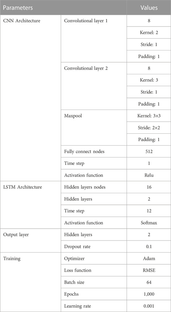
TABLE 2. Setting of hyperparameters.

3.1.3 Results and comparison

The evaluation results for LSTM-M and MPM are shown in Table 3, and the boldface indicates better performance.

TABLE 3

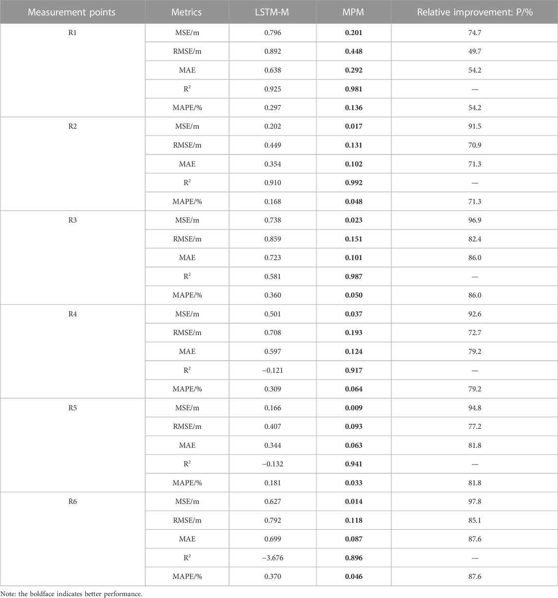
TABLE 3. Evaluation results of prediction models.

The intuitive comparison results are shown in Figure 6. It can be seen from the figure that both models can achieve simultaneous predictions of multiple parallel targets, but the MPM model performs better, and the prediction accuracy is greatly improved compared to the LSTM-M model. From the MAPE, MSE, RMSE, and MAE, it can be seen that the MPM model improves on average by 76.7%, 91.4%, 73.0%, and 76.7%, respectively, compared to the LSTM-M model. According to R², the MPM model has a good fit between predictions and target values, and the average R² for the six measurement points is 0.952. The results show that the prediction accuracy has been remarkably improved by introducing the CNN model. It is very important to consider latent correlation features between target values based on the benchmark LSTM-M model.

FIGURE 6

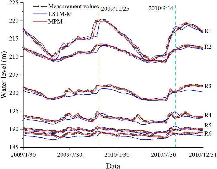
FIGURE 6. Measurement and predicted values from LSTM-M and MPM.

In addition, it can be seen from the predictions that the errors of the two models are mainly reflected at the time when the inflection point fluctuates greatly and the MPM model has more ideal feature sensitivity. For example, in Figure 6, the data at both times of the dashed lines indicate that the rules learned by the LSTM-M model are approximately the same, which is the delayed peak, especially at R1, R4, and R5 on 14 September 2010, where the predicted values differ significantly from target values. As can be seen, it is difficult to guarantee the accuracy of LSTM-M predictions when there are differences in the correlation between environmental variables and various target values. In addition, during the training process, because the same parameters are used for each measurement value of the LSTM-M model, the parameters are adjusted by errors and back propagation of multiple measurement points. When the error of one measurement point is large, the prediction accuracy of other measurement points will be sacrificed to balance the overall error. The CNN model is introduced to extract latent correlation features between adjacent target values, consider correlations and differences between target values, and adopt different parameters accordingly, thus improving the learning effect of the model and effectively enhancing the prediction performance.

3.2 The second model application

3.2.1 Project status and monitoring data profile

Lubuge is a weathered rockfill dam, with the top elevation of the dam, the maximum dam height, the width of the dam crest, and the length of the dam crest being 1138.0, 103.8, 10.0, and 217.0 m, respectively. The normal reservoir water level is 1130.0 m, the corresponding storage capacity is 111.0 million m³, the dead water level is 1105.0 m, the storage capacity is 75.0 million m³, and the reservoir presents an incomplete capacity for seasonal regulation. Given the low downstream water level and little fluctuation, the influence of the downstream water level is not considered in this case. Three osmometers from the largest section were selected for analysis and were denoted R1–R3. The position of multiple osmometers is shown in Figure 7.

FIGURE 7

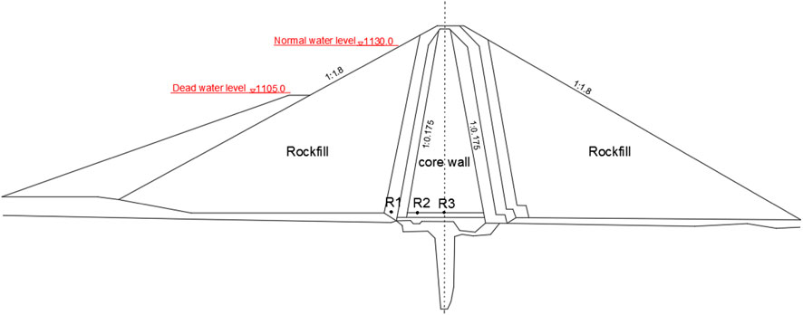
FIGURE 7. Osmometers distribution of the Lubuge rockfill dam.

3.2.2 Training and prediction

There were 1,375 observations from 17 May 2009 to 19 February 2013. The time series of monitoring data is shown in Figure 8.

FIGURE 8

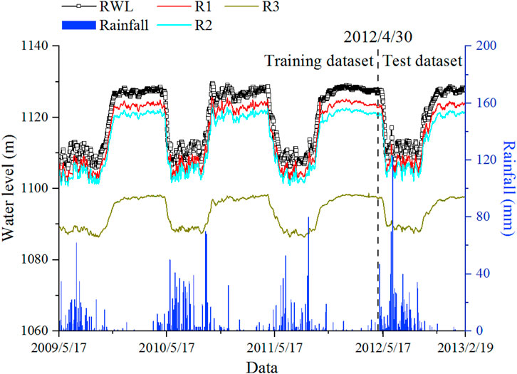
FIGURE 8. Time series of monitoring data.

The dataset from 17 May 2009 to 30 April 2012, is used as training data for optimizing and adjusting parameters, and the dataset from 1 May 2012 to 19 February 2013, is used as test data for prediction and performance evaluation.

In this case, the CNN model has three convolutional layers with 16, 8, and 8 neurons and 2, 2, and 3 convolution kernels, respectively. The LSTM model has three hidden layers with 128 neurons. The batch size is 32, and the other parameters are the same as those above. The details are shown in Table 4.

TABLE 4

TABLE 4. Setting of hyperparameters.

3.2.3 Results and comparison

The evaluation results for LSTM-M and MPM are shown in Table 5, and the boldface indicates better performance.

TABLE 5

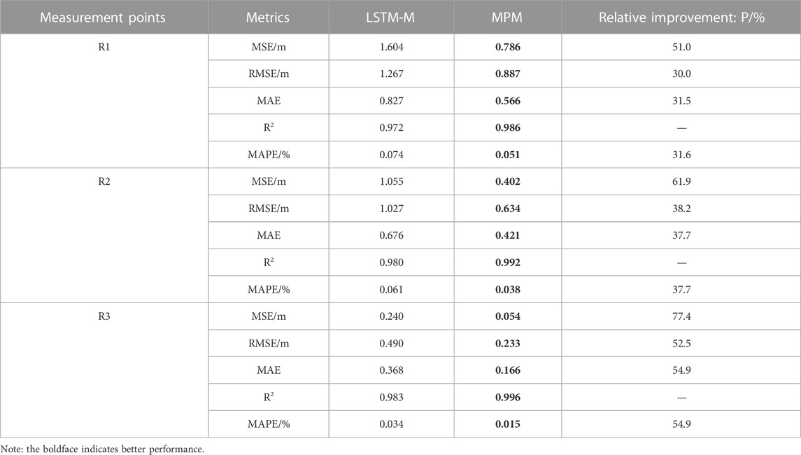
TABLE 5. Evaluation results of prediction models.

The intuitive comparison results are shown in Figure 9. When LSTM-M and MPM are compared, it is clear that the prediction accuracy of MPM has improved significantly, and MSE, RMSE, MAE, and MAPE have improved by 63.4%, 40.2%, 41.4%, and 41.4% on average, at the three measurement points, respectively. The average R² at the three measurement points is 0.992, which is higher than that of LSTM-M (0.978).

FIGURE 9

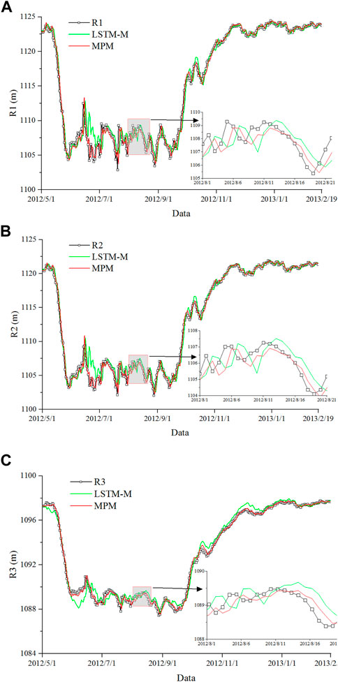
FIGURE 9. Measurement and predicted values from LSTM-M and MPM. (A) R1. (B) R2. (C) R3.

3.3 Result analysis

The MPM model has achieved better prediction results in practical applications, and possible reasons for this include: 1. The LSTM model can deeply learn the non-linear temporal features between environmental variables and target values. 2. The introduction of the CNN model can effectively obtain latent correlation features between target values, and when the causal relationship between target values and environmental variables is different, the latent correlation features can be effectively used to reduce the prediction error and better fit the variation trend. 3. Feature fusion can act as feature reinforcement and intercorrelation, allowing data features to be extracted and identified from various aspects. 4. Multi-target joint training implicitly increases the amount of training data and prevents model over-fitting.

4 Conclusion

In this study, the MPM model is proposed, which considers causal temporal features between environmental variables and target values, as well as correlations and differences between target values.

The MPM model integrates CNN and LSTM into a unified framework. The LSTM model is introduced to efficiently learn the causal temporal features of short-term time changes and long-periodic variation rules in time series, while the CNN model is introduced to build the soft parameter sharing layer to efficiently mine latent correlation features of the data grid at each moment. After integrating causal temporal features and latent multi-target correlation features, fully connected layers are used to establish the mapping relationship between the comprehensive feature vector and the multi-target outputs. The MPM model allows data features to be extracted and identified from various aspects. Monitoring data of two embankment dams are used to show the prediction performance. Compared with the traditional benchmark model based on hard parameter sharing, the MPM model has better fitting effect and prediction accuracy.

The main advance of the MPM model is that CNN and LSTM are combined parallelly. Parallel networks do not depend on each other, which improves the prediction the performance of the model without consuming too much time. Although the monitoring data at multiple points in this paper are the same type, the proposed MPM model is still applicable in prediction of multiple types of physical fields in safety monitoring.

It should be noted that the model performance is inspected on the basis of the training data, which is during the normal operation period of the embankment dams. Further studies are needed to test the model performance based on the data of other types of dams and on the data of different periods of monitoring data, such as the initial operation data or long-term operation data.

Data availability statement

The original contributions presented in the study are included in the article/supplementary material, further inquiries can be directed to the corresponding author.

Author contributions

YW, GD, WH, YZ, and XW conceived of the presented idea. GD and WH set up the prediction model and performed the computations. GD analyzed the data. YW supervised the study. WH and GD wrote the first version of the manuscript. All authors contributed to manuscript revision, read, and approved the submitted version.

Funding

This work was supported by the National Key Research and Development Program of China (Grant No. 2022YFC3005501), the IWHR Research and Development Support Program (Grant No. GE0145B032021), and the Independent Research Fund of State Key Laboratory of Simulation and Regulation of Water Cycle in River Basin (Grant No. SKL2020ZY09).

Conflict of interest

The authors declare that the research was conducted in the absence of any commercial or financial relationships that could be construed as a potential conflict of interest.

Publisher’s note

All claims expressed in this article are solely those of the authors and do not necessarily represent those of their affiliated organizations, or those of the publisher, the editors and the reviewers. Any product that may be evaluated in this article, or claim that may be made by its manufacturer, is not guaranteed or endorsed by the publisher.

References

Azarafza, M., Azarafza, M., Akgün, H., Atkinson, P. M., and Derakhshani, R. (2021). Deep learning-based landslide susceptibility mapping. Sci. Rep. 11 (1), 24112. doi:10.1038/s41598-021-03585-1

PubMed Abstract | CrossRef Full Text | Google Scholar

Azarafza, M., Hajialilue Bonab, M., and Derakhshani, R. (2022). A deep learning method for the prediction of the index mechanical properties and strength parameters of marlstone. Materials 15 (9), 6899. doi:10.3390/ma15196899

PubMed Abstract | CrossRef Full Text | Google Scholar

Bonelli, S., and Royet, P. (2001). “Delayed response analysis of dam monitoring data[C],” in Proceedings of ICOLD European symposium (Oxfordshire: Taylor and Francis Press), 91–99.

Google Scholar

Caruana, R. A. (1993). Multitask learning: A knowledge-based source of inductive bias[J]. Mach. Learn. Proc. 10 (1), 41–48. doi:10.1016/b978-1-55860-307-3.50012-5

CrossRef Full Text | Google Scholar

Chen, Y., Ma, G., Zhou, W., Wu, J. Y., and Zhou, Q. C. (2022). Rockfill dam deformation prediction model based on deep learning extracting spatiotemporal features[J]. J. Hydroelectr. Eng. 2022, 1–13.

Google Scholar

Deng, G., Cao, K., Chen, R., Wen, Y. F., Zhang, Y. Y., and Chen, Z. K. (2020). A new method for dynamically estimating long-term seepage failure frequency for high concrete faced rockfill dams. Environ. Earth Sci. 79 (10), 247. doi:10.1007/s12665-020-08962-z

CrossRef Full Text | Google Scholar

Deng, N. W., Chen, Z., and Ye, Z. R. (2007). Modeling of partial least-squared regression and genetic algorithm in dam safety monitoring analysis[J]. Dam Saf. 4, 33–35. doi:10.3969/j.issn.1671-1092.2007.04.011

CrossRef Full Text | Google Scholar

Fanelli, M. (1975). Control of dam displacements. Energ. Elettr. 52, 125–139.

Google Scholar

Foster, M., Fell, R., and Spannagle, M. (2000). The statistics of embankment dam failures and accidents. Rev. Can. De. Géotechnique. 37 (5), 1000–1024. doi:10.1139/t00-030

CrossRef Full Text | Google Scholar

Gao, Y., She, Q., Ma, J., Zhao, M., and Yuille, A. L. (2019). “Nddr-cnn: Layer-wise feature fusing in multi-task cnn by neural discriminative dimensionality reduction[C],” in Proceedings of the IEEE Conference on Computer Vision and Pattern Recognition, Long Beach, CA, USA, 3205–3214. doi:10.48550/arXiv.1801.08297

CrossRef Full Text | Google Scholar

Gu, C. S., Su, H. Z., and Wang, S. W. (2016). Advances in calculation models and monitoring methods for long-term deformation behavior of concrete dams[J]. J. Hydroelectr. Eng. 35 (5), 1–14. doi:10.11660/slfdxb.20160501

CrossRef Full Text | Google Scholar

Gu, C. S., Wang, Y. C., Peng, Y., and Xu, B. S. (2011). Ill-conditioned problems of dam safety monitoring models and their processing methods. Sci. China Technol. Sci. 54 (12), 3275–3280. doi:10.1007/s11431-011-4573-z

CrossRef Full Text | Google Scholar

Hakim, W. L., Rezaie, F., Nur, A. S., Panahi, M., Khosravi, K., Lee, C. W., et al. (2021). Convolutional neural network (CNN) with metaheuristic optimization algorithms for landslide susceptibility mapping in Icheon, South Korea. J. Environ. Manag. 305, 114367. doi:10.1016/j.jenvman.2021.114367

CrossRef Full Text | Google Scholar

Hochreiter, S., and Schmidhuber, J. (1997). Long short-term memory. Neural Comput. 9 (8), 1735–1780. doi:10.1162/neco.1997.9.8.1735

PubMed Abstract | CrossRef Full Text | Google Scholar

Hochreiter, S. (1998). The vanishing gradient problem during learning recurrent neural nets and problem solutions. Int. J. Uncertain. Fuzziness Knowledge-Based Syst. 6 (2), 107–116. doi:10.1142/S0218488598000094

CrossRef Full Text | Google Scholar

Hou, W. Y., Wen, Y. F., Deng, G., Zhang, Y. Y., and Chen, H. (2022). Deformation prediction of high embankment dams by combining time series decomposition and deep learning[J]. J. Hydroelectr. Eng. 41 (3), 123–132. doi:10.11660/slfdxb.20220312

CrossRef Full Text | Google Scholar

Hua, G. W., Wang, S. J., Xiao, M., and Hu, S. H. (2023). Research on the uplift pressure prediction of concrete dams based on the CNN-gru model. J. Water. 15 (2), 319. doi:10.3390/w15020319

CrossRef Full Text | Google Scholar

Huang, H., and Chen, B. (2012). Dam seepage monitoring model based on dynamic effect weight of reservoir water level. Energy Procedia 16, 159–165. doi:10.1016/j.egypro.2012.01.027

CrossRef Full Text | Google Scholar

Hubel, D. H., and Wiesel, T. N. (1959). Receptive fields of single neurones in the cat's striate cortex. J. Physiology 148 (3), 574–591. doi:10.1113/jphysiol.1959.sp006308

CrossRef Full Text | Google Scholar

Jeon, J., Lee, J., Shin, D., and Park, H. (2009). Development of dam safety management system. Adv. Eng. Softw. [J] 40 (8), 554–563. doi:10.1016/j.advengsoft.2008.10.009

CrossRef Full Text | Google Scholar

Krizhevsky, A., Sutskever, I., and Hinton, G. E. (2012). ImageNet classification with deep convolutional neural networks[J]. Adv. neural Inf. Process. Syst. 52, 1097–1105. doi:10.1145/3065386

CrossRef Full Text | Google Scholar

LeCun, Y., and Bengio, Y. (1995). Convolutional networks for images, speech, and time series[J]. Handb. Brain Theory Neural Netw. 3361 (10).

Google Scholar

Li, Y. T., Bao, T. F., Gao, Z. X., Shu, X. S., Zhang, K., Xie, L. C., et al. (2022). A new dam structural response estimation paradigm powered by deep learning and transfer learning techniques. Struct. Health Monit. 21 (3), 770–787. doi:10.1177/14759217211009780

CrossRef Full Text | Google Scholar

Liang, X., Tang, S. B., Tang, C. A., Hu, L. H., and Chen, F. (2022). Influence of water on the mechanical properties and failure behaviors of sandstone under triaxial compression. Rock Mech. Rock Eng. 56, 1131–1162. doi:10.1007/s00603-022-03121-1

CrossRef Full Text | Google Scholar

Misra, I., Shrivastava, A., and Gupta, A. (2016). “Hebert M. Cross-stitch networks for multi-task learning[C],” in Proceedings of the 2016 IEEE Conf on Computer Vision and Pattern Recognition, Las Vegas, 3994–4003. IEEE. doi:10.1109/CVPR2016.433

CrossRef Full Text | Google Scholar

Nikoobakht, S., Azarafza, M., Akgün, H., and Derakhshani, R. (2022). Landslide susceptibility assessment by using convolutional neural network. Appl. Sci. 12, 5992. doi:10.3390/app12125992

CrossRef Full Text | Google Scholar

Qu, X. D., Yang, J., and Chang, M. (2019). A deep learning model for concrete dam deformation prediction based on RS-LSTM. J. Sensors 1, 1–14. doi:10.1155/2019/4581672

CrossRef Full Text | Google Scholar

Ren, Q., Li, M., Li, H., and Shen, Y. (2021). A novel deep learning prediction model for concrete dam displacements using interpretable mixed attention mechanism. Adv. Eng. Inf. 50 (3), 101407. doi:10.1016/j.aei.2021.101407

CrossRef Full Text | Google Scholar

Shi, Z. W., Gu, C. S., Zhao, E. F., and Xu, B. (2020). A novel seepage safety monitoring model of CFRD with slab cracks using monitoring data. Math. Problems Eng. 12, 1–13. doi:10.1155/2020/1641747

CrossRef Full Text | Google Scholar

Su, H. Z., Gu, C. S., and Wu, Z. R. (2000). Application of artificial intelligence theory to dam safety monitoring[J]. Dam Observation Geotechnical Tests 24 (3), 7–9. doi:10.3969/j.issn.1671-3893.2000.03.003

CrossRef Full Text | Google Scholar

Su, H. Z., Wu, Z. R., Wen, Z. P., and Gu, C. S. (2001). Dam safety monitoring model based on fuzzy neural network and genetic algorithm[J]. Dam Observation Geotechnical Tests 25 (1), 10–12+22. doi:10.3969/j.issn.1671-3893.2001.01.004

CrossRef Full Text | Google Scholar

Sun, L. C. (2012). Study on the seepage flow prediction of earth-rock dam [D]. Nanning: Guangxi university. (in Chinese).

Google Scholar

Sun, Q. K., Wang, X. J., Zhang, Y. Z., Zhang, F., Zhang, P., and Gao, W. Z. (2021). Multiple load prediction of integrated energy system based on long short-term memory and multi-task learning[J]. Automation Electr. Power Syst. 45 (5), 63–70.

Google Scholar

Tang, S. B., Li, J. M., Ding, S., and Zhang, L. (2022). The influence of water-stress loading sequences on the creep behavior of granite. Bull. Eng. Geol. Environ. 81, 482. doi:10.1007/s10064-022-02987-3

CrossRef Full Text | Google Scholar

Wan, C., Li, W. Z., Ding, W. X., Zhang, Z. J., Lu, Q. N., Qian, L., et al. (2021). Multi-task sequence learning for performance prediction and KPI mining in database management system. Inf. Sci. 568, 1–12. doi:10.1016/j.ins.2021.03.046

CrossRef Full Text | Google Scholar

Wu, Z. R., and Su, H. Z. (2005). Dam health diagnosis and evaluation. Smart Mater. Struct. 14 (3), S130–S136. doi:10.1088/0964-1726/14/3/016

CrossRef Full Text | Google Scholar

Xu, D., Shi, Y. X., Tsang, I. W., Ong, Y. W., Gong, C., and Shen, X. B. (2019). Survey on multi-output learning. IEEE Trans. Neural Netw. Learn. Syst. 31, 2409–2429. doi:10.1109/TNNLS.2019.2945133

PubMed Abstract | CrossRef Full Text | Google Scholar

Yan, R., Geng, G. C., Jiang, Q. Y., and Li, Y. L. (2019). Fast transient stability batch assessment using cascaded convolutional neural networks. IEEE Trans. Power Syst. 34 (4), 2802–2813. doi:10.1109/TPWRS.2019.2895592

CrossRef Full Text | Google Scholar

Yang, D. S., Gu, C. S., Zhu, Y. T., Dai, B., Zhang, K., Zhang, Z. D., et al. (2020). A concrete dam deformation prediction method based on LSTM with attention mechanism. IEEE Access 8, 185177–185186. doi:10.1109/access.2020.3029562

CrossRef Full Text | Google Scholar

Yang, J., Qu, J., Mi, Q., and Li, Q. (2020). A CNN-LSTM model for tailings dam risk prediction. IEEE Access 8, 206491–206502. doi:10.1109/ACCESS.2020.3037935

CrossRef Full Text | Google Scholar

Yao, K. F., Wen, Z. P., Yang, L. P., Chen, J., Hou, H. W., and Su, H. Z. (2022). A multipoint prediction model for nonlinear displacement of concrete dam. Computer-Aided Civ. Infrastructure Eng. 37 (14), 1932–1952. doi:10.1111/mice.12911

CrossRef Full Text | Google Scholar

Zhang, J. B., Zheng, Y., and Qi, D. K. (2017). “Deep spatio-temporal residual networks for citywide crowd flows prediction[C],” in Proceedings of the thirty-first AAAI conference on artificial intelligence (AAAI'17) (Palo Alto, California, U.S. AAAI Press), 1655–1661. doi:10.48550/arXiv.1610.00081

CrossRef Full Text | Google Scholar

Zhang, L., Cai, Y. Y., Huang, H. L., Li, A. Q., Yang, L., and Zhou, C. H. (2022). A CNN-LSTM model for soil organic carbon content prediction with long time series of MODIS-based phenological variables. Remote Sens. 14 (18), 4441. doi:10.3390/rs14184441

CrossRef Full Text | Google Scholar

Zhao, M. D., Jiang, H. F., Zhao, M. D., and Bie, Y. J. (2021). Prediction of seepage pressure based on memory cells and significance analysis of influencing factors. Complexity 12, 1–10. doi:10.1155/2021/5576148

CrossRef Full Text | Google Scholar

Zhou, Y., Chang, F. J., Chang, L. C., Kao, I. F., and Wang, Y. S. (2018). Explore a deep learning multi-output neural network for regional multi-step-ahead air quality forecasts. J. Clean. Prod. 209 (1), 134–145. doi:10.1016/j.jclepro.2018.10.243

CrossRef Full Text | Google Scholar

Zhu, C., Xu, X. D., Wang, X. T., Xiong, F., Tao, Z. G., Lin, Y., et al. (2019). Experimental investigation on nonlinear Flow anisotropy behavior in fracture media. Geofluids 9, 1–9. doi:10.1155/2019/5874849

CrossRef Full Text | Google Scholar

Zong, M., Wang, R. L., Ma, Y. J., and Ji, W. T. (2022). Spatial and temporal saliency based four-stream network with multi-task learning for action recognition. Appl. Soft Comput. 132, 109884. doi:10.1016/j.asoc.2022.109884

CrossRef Full Text | Google Scholar