Machine learning approaches to estimation of the compressibility of soft soils

The modulus of compression and coefficient of compressibility of soft soils are key parameters for assessing deformation of geotechnical infrastructure. However, the consolidation tests used to determine these two indices are time-consuming and the results are easily and heavily influenced by workmanship, testing apparatus, and other factors. Therefore, it is of great interest to develop a simple approach to accurately estimate these compressibility indices. This article presents the development of three machine learning (ML) models—at artificial neural network (ANN), a random forest model, and a support vector machine model—for mapping of the two compressibility indices for soft soils. A database containing 743 sets of measured physical and compression parameters of soft soils was adopted to train and validate the models. To quantify model uncertainty, the accuracies of the ML models were statistically evaluated using a bias factor defined as the ratio of the measured to the predicted compression indices. The results showed that all three ML models were accurate on average, with low dispersion in prediction accuracy. The ANN was found to be the best model, as it provides a simple analytical form and has no hidden dependency between the bias and predicted indices. Finally, the probability distribution functions of the bias factors were also determined using the fit-to-tail technique. The results of this study will be helpful in saving cost and time in geotechnical investigation of soft soils.

1 Introduction

The Guangdong–Hong Kong–Macao Greater Bay Area (GBA) in China is undergoing ongoing and extensive infrastructure construction. Due to the widely distributed marine sedimentary soft soils in the GBA, geotechnical infrastructure resting on soft soils is usually challenged by both excessive deformation and insufficient bearing capacity throughout the lifetime of service. To assess infrastructure deformation, a set of laboratory and in situ tests (Bo et al., 2018; Orense et al., 2018) must be routinely performed in order to determine both the physical and the mechanical properties of the soil for projects in soft soil areas. For example, consolidation tests (Zabielska and Katarzyna, 2018) are conducted to study the compressibility of soft soils and consolidation is typically quantified by two indices, namely, the modulus of compression and the coefficient of compressibility.

While consolidation tests are a routine type of geotechnical laboratory test, they have several drawbacks in cases of soft soil. First, the tests can be very time-consuming (Holtz et al., 2010) and costly, especially for multi-stage consolidations. Second, sample disturbance is usually unavoidable when transporting soft soils from sites to the laboratory. These disturbances can result in significant alterations of soil structures and, thus, the compressibility (Lunne et al., 2006). Finally, errors relating to testing apparatus are also uncontrollable.

Due to these drawbacks, the development of a simple, practical, and sufficiently accurate equation to rapidly assess soil compressibility indices is highly desirable. Koppula (1981) used the least squares technique to regress the physical parameters of soft clays against their compression indices. Empirical regressions are applicable to estimate the settlement of structures resting on cohesive soils. Amiri et al. (2018) used multiple linear regression to estimate unsaturated shear strength parameters using several indices of the physical properties of soil as function inputs. Liu et al. (2018) reported on the relationships between the mechanical properties of clays and temperature. Motaghedi and Eslami (2014), Mcgann et al. (2015), Cao and Wang (2013), Lim et al. (2020), and Schneider et al. (2008) empirically linked data from CPT on sleeve friction, cone tip resistance, and porewater pressure data to soil properties including cohesion, friction angle, soil classification, overconsolidation ratio, and shear wave velocity. Yoon et al. (2004) and Yan et al. (2009) proposed empirical correlations of compression index for marine clay based on regression analysis and Bayesian inference. Finally, Cao et al. (2019) determined soil stratigraphy using a Bayesian method based on CPT.

While the development of empirical equations using traditional regression approaches to predict the mechanical properties of soils has facilitated geotechnical analyses to a large extent, it remains challenging to establish accurate correlations, owing to the major uncertainty in and great complexity of soil properties (Ching and Phoon, 2014). Over the past decades, the applicability of machine learning (ML) approaches, such as artificial neural networks (ANNs), random forest (RF) methods, and support vector machines (SVMs), among others, has been well-proven in terms of their ability to efficiently and accurately map highly non-linear problems in a wide variety of areas of engineering (Arditi and Pulket, 2010; Chen et al., 2021), including geotechnical engineering. Successful examples of applications include analyses of slope stability (Kardani et al., 2021; Meng et al., 2021) and deformation (Zhang et al., 2019; Zhang et al., 2020a; Zhang W et al., 2021); pile designs (Makasis et al., 2018; Zhang et al., 2020e); prediction of the bearing capacity of strip footings (Acharyya, 2019; Sadegh et al., 2021); lateral wall deformation and basal heave stability for braced excavations (Goh et al., 1995; Zhang et al., 2020); soil constitutive relations (Najjar and Huang, 2007); liquefaction resistance of sands (Kim and Kim, 2006); lining response for tunnels (Zhang et al., 2020g); calibration of resistance factors for reliability-based load and resistance factor design (Hu and Lin, 2019); prediction of soil transparency (Wang et al., 2021); analysis of ground settlement induced by shield tunneling (Zhang et al., 2020c); reliability analysis by SVM (Pan and Dias, 2017); and mapping of groundwater potential using SVM, RF, and GA models (Naghibi et al., 2017), among others. In addition to solving geotechnical analysis problems, these ML approaches have also achieved success in mapping from the physical parameters of soil to the mechanical parameters. Moreover, Park, and Lee (2011), Pham et al. (2019a), Pham et al. (2019), and Zhang et al. (2020f) studied the compressibility feature of soils using ML techniques. Das et al. (2011), Kanungo et al. (2014), Kiran et al. (2016), Pham et al. (2018), and Zhang L et al. (2021) developed ML models to estimate the shear strength parameters of soils under various conditions. Çelik and Tan (2005) and Samui et al. (2008) determined preconsolidation pressure using an ANN and an SVM method, respectively. For details of additional applications, readers are also referred to the state-of-the-art reviews of ML applications in geotechnical and geoscience engineering areas conducted by Shahin Mohammad (2016), Moayedi et al. (2019), Zhang and Ching et al. (2021), Zhang et al. (2020f), and Hou et al. (2021).

Although the development of ML models of soil mechanical parameters remains a hot topic that continues to attract attention, few studies have reported employed bias statistics for quantification of model uncertainty. Most previous studies have used the mean absolute error (MAE), root mean square error (RMSE), and coefficient of determination ($R^2$) to characterize model accuracy. However, we offer a reminder that a lack of model bias statistics (i.e., the mean, coefficient of variation (COV), and probability distribution function) makes it difficult to make use of ML models in reliability-based analysis and design.

The present study first introduces a large database consisting of 743 sets of measured physical property parameters and compressibility indices based on laboratory tests for soft soils sampled from a city in the GBA of China. The main physical property parameters are water content, density, and void ratio. The compressibility indices for the soils are the modulus of compression and the coefficient of compressibility. Next, a set of ML techniques (ANN, RF, and SVM) are adopted to develop useful models for efficient and accurate mappings from the three aforementioned common physical parameters to the two compressibility indices. Finally, the model uncertainties of the proposed ML models are evaluated, where model uncertainty is quantitatively defined by the statistics of the bias factor, defined as the ratio of the measured to predicted compression indices. The probability distributions of the model biases are also investigated. The performance of each of the machine learning models developed is discussed and the models are compared on performance. The results of this study demonstrate the feasibility of applying ML techniques to make prompt assessments of the compressibility of soft soils in the GBA area based on simple physical properties of the soil.

2 Methodology

The methodology used in this study consisted of two parts. The first was model development, in which several ML models (ANN, RF, and SVM) were developed. The second was model evaluation using the model bias method (Ching and Schweckendiek, 2021; Jin et al., 2018). In model development, the physical properties of the soils were used as inputs to the ML models and the mechanical properties were the targets. The main physical parameters were water content, void ratio, and density of soft soil. The mechanical parameters were compression indices obtained from compression (CP) tests. The database is introduced in Section 3.

Typically, the MSE is used as an indicator of the accuracy of machine learning models. However, the MSE is not sufficient to fully capture model uncertainty. Therefore, the present study adopted the model bias method described below for the characterization of the model uncertainty of the machine learning models. The bias is defined as the ratio of the measured to the predicted value. Technical details of the machine learning models and the model bias method are provided in this section.

2.1 Artificial neural network technique

The use of ANNs is widely accepted as a technique that is capable of efficiently handling almost any regression or classification problem given sufficient data. Structurally, an ANN consists of an input layer, several hidden layers, and an output layer (Figure 1A). The learning process of an ANN includes forward propagation of information and backpropagation to adjust the error (Rafiq et al., 2001). Figure 1B illustrates how a neuron transmits information in ANN forward propagation. Suppose there are m neurons in hidden layer k, denoted as $n_1^k$, $n_2^k$,…, $n_m^k$ (the neurons in the input layer can be denoted as $n_i^0$). Then, the $t^{\mathrm{t}\mathrm{h}}$ neuron in hidden layer k+1, denoted as $n_t^{k+1}$, is calculated as (Haykin, 2009):

$n_t^{k+1}=f\left(z_t^{k+1}\right)=f\left({\displaystyle \sum _{i=1}^{i=m}}{w}_{t,i}^k{n}_i^k+b_t^{k+1}\right).(1)$

FIGURE 1

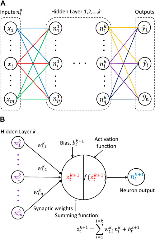
FIGURE 1. Construction of an ANN: (A) layered network; (B) artificial neuron.

$n_t^{k+1}$ is computed in two steps: first, a summing function $z_t^{k+1}={\displaystyle \sum _{i=1}^{i=m}}{w}_{t,i}^k{n}_i^k+b_t^{k+1}$ is computed, where $w_{t,i}^k$ is the weight representing the strength of the connection between the neurons $n_i^k$ and $n_t^{k+1}$. The connection strength is positively correlated with the value of the weight. Parameter $b_t^{k+1}$ is the bias. Step two is to substitute $z_t^{k+1}$ into the activation function $f\left(x\right)$ as $f\left(z_t^{k+1}\right)$ to solve non-linear mapping problems. Commonly adopted functions for $f\left(x\right)$ are the “tanh,” “sigmoid,” and “ReLu” functions. Haykin (2009)discusses the selection of activation functions for different mapping scenarios with ANN models.

The difference between the outputs (each predicted value ${\widehat{y}}_p$) and the targets (each measured value $y_m$) is called the error and is defined as $\mathrm{\epsilon }={\widehat{y}}_p-y_m$. Backpropagation is employed to tune the weights $w$ and biases $b$ until ${\mathrm{\epsilon }}^2$ is minimized. This value of ${\mathrm{\epsilon }}^2$, which can be expressed as ${\mathrm{\epsilon }}^2={\sum }_1^k{\epsilon }_k^2/k={\sum }_1^k{\left({\widehat{y}}_{p,k}-y_{m,k}\right)}^2/k$, is referred to as the mean squared error (MSE).

The input data are usually randomly divided into three subsets in the development of an ANN model: training, validation, and test sets. The same process is carried out for each set of the target (measured) data. The training set is used to determine the weights and biases of the neurons, and the validation set is utilized to prevent overfitting problems during the training process. Hence, the optimal weights and biases that minimize ${\mathrm{\epsilon }}^2$ are determined using both the training and the validation sets together. The test data are used to evaluate the learning effectiveness of the ANN model. If this is unsatisfactory, the ANN model requires further optimization through adjustment of the hidden layers or the numbers of neurons, use of different activation functions or training algorithms, or other changes. Additional technical aspects of the ANN method are described by Rafiq et al. (2001), Haykin (2009), and Demuth et al., 2014.

2.2 Random forest technique

The random forest method is an ensemble learning method that provides solutions for classification and regression problems. The main idea is to grow a number of decision trees through bagging and random feature selection. Each decision tree has high variance and thus is often rather poor in generalization. As illustrated in Figure 2, the RF regression model is constructed by assembling several individual decision trees, and predictions are made by averaging. Note that the generalization ability of the classification model is improved by voting. The “forest” reduces the variance by averaging and greatly enhances prediction accuracy.

FIGURE 2

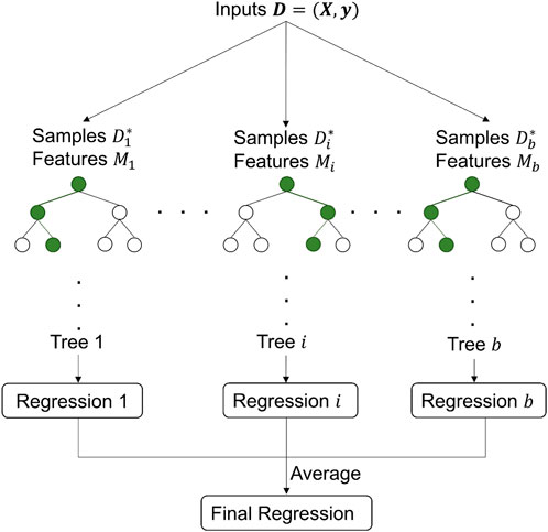
FIGURE 2. Diagram of a random forest regression model.

Suppose a training dataset $\mathit{D}=\left(\mathit{X},\mathit{y}\right)$, where $\mathit{X}$ is an $n\times p$ data matrix and $\mathit{y}$ is the corresponding $n$-vector. The data not in the training dataset at each bootstrap can be referred to as “out-of-bag” (OOB). Normally, the RF algorithm is as follows (Efron and Hastie, 2016):

Step 1:. Select the number of trees $B$ and random features m $\le p$; typically, $m=\sqrt{p}$ or $p/3$;

Step 2:. Bootstrap a subset of $\mathit{D}$ by randomly sampling $n$ rows with replacement $B$ times, denoted as ${\mathit{D}}_i^{*}$;

Step 3:. Develop a tree ${\widehat{r}}_i\left(x\right)$ to its maximum depth using ${\mathit{D}}_i^{*}$ at each node in ${\widehat{r}}_i\left(x\right)$, sampling $m$ of the $p$ features to make each split;

Step 4:. Bag these trees and take the average at any point $x_0$. The resulting RF prediction can be expressed as

${\widehat{r}}_{RF}\left(x_0\right)=\frac{1}{B}{\displaystyle \sum _{i=1}^{i=b}}{\widehat{r}}_i\left(x_0\right).(2)$

Step 5:. At each bootstrap, compute the OOB error for each response observation.The aggregate OOB error is obviously the average of each individual OOB error. The OOB error is a performance indicator that can be used to test the generalization ability of the RF model; hence, no cross-validation or additional testing set is required. The RF model can be optimized by adjusting the parameters $B$ and $m$ if the overall OOB estimate of error does not meet the prescribed threshold value. Additional technical details on RF models can be found in, e.g., Breiman (2001), Efron and Hastie (2016), and Liaw and Wiener (2002).

2.3 Support vector machines

The SVM method is a classifier in which the main idea is to establish a classification hyperplane as a decision surface. As shown in Figure 3, the optimal separating hyperplane is the classification hyperplane $\omega x+b=0$ that creates the largest margin between the hyperplane and the nearest data. In more recent applications involving regression and time series prediction, SVMs have also shown excellent performance (Drucker et al., 1997; Müller et al., 1997). As with classification, the goal of SVM regression is to identify an optimal separating hyperplane function $f_{SV}\left(x\right)$ that creates the largest margin between targets for all the training dataset and is also as flat as possible (Efron and Hastie, 2016). Assume function $f_{SV}\left(x\right)$ is a linear function with the following form:

$f_{SV}\left(x\right)={\omega }_s^T{\varphi }_s\left(x\right)+b,(3)$

FIGURE 3

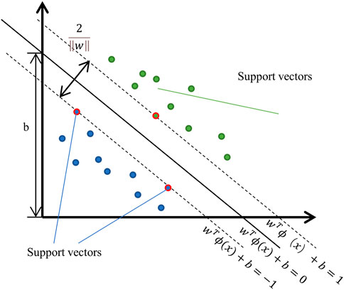
FIGURE 3. Diagram of a support vector machine model.

where ${\varphi }_s\left(x\right)$ is a set of mapping functions that connect the source data to a high-dimensional feature space, ${\omega }_s$ is the weight, and $b$ is the threshold. Flatness in Eq. (3) means that the SVM regression problem is equivalently reformulated as a convex optimization problem with a target of minimizing ${\omega }^2$; it can be written as by Smola and Schölkopf (2004):

$\begin{array}{c}\mathrm{m}\mathrm{i}\mathrm{n}\mathrm{i}\mathrm{m}\mathrm{i}\mathrm{z}\mathrm{e}\frac{1}{2}\Vert {\omega }_s^2\Vert \\ \mathrm{s}\mathrm{u}\mathrm{b}\mathrm{j}\mathrm{e}\mathrm{c}\mathrm{t}\mathrm{t}\mathrm{o}\left|y_i-{\omega }_s{\varphi }_s\left(x\right)-b\right|\le \epsilon .\end{array}(4)$

Equation (4) implicitly assumes that mapping precision $\epsilon$ does in fact exist for the function $f_{SV}\left(x\right)$. In SVM models, different ø functions are generally used to construct classifiers with satisfactory performance. For highly non-linear cases, kernel functions are used to expand ø and enhance its mapping ability. The present study adopts a Gaussian kernel function (i.e., a radial basis function) with an exponentially decaying function for $\varphi$, consistent with most studies in the literature, e.g., Scholkopf et al. (1997), Krishnan et al. (2018), Mangalathu and Jeon (2018), and Scholkopf and Smola (2018). The technical details of SVMs are described by Scholkopf et al. (1997), Smola and Schölkopf (2004), and Scholkopf and Smola (2018).

2.4 Characterization of model uncertainty

Bias statistics proposed in model bias methods, such as the bias mean, bias coefficient of variation (COV), and bias probability distribution, have been widely employed to characterize model uncertainty. In this study, the predicted values were the outputs of the machine learning models, while the measured values were available directly from the database. The bias mean represents the average accuracy of the model, while the bias COV represents the dispersion in prediction accuracy. The bias probability distribution is used as an input to reliability-based analyses of machine learning models. Lastly, the randomness of the bias also needs to be checked.

3 Database of soft soil properties

The database of compression indices of soil soft established by Lin et al. (2022) was used in the present study for the development of the machine learning models. For completeness, the database is briefly re-described here.

The database consists of 743 sets of physical properties and corresponding compression indices for soft soils. Soft soil samples were obtained from Shenzhen, a major megacity in China. The physical parameters of moisture content ($\omega$), density ($\rho$), and void ratio ($e$) were obtained through a succession of geotechnical tests. The compression indices (i.e., modulus of compression $E_S$ and coefficient of compressibility $\alpha$) were derived from soil compression (CP) tests. On the basis of these data, a 743 $\times$ 3 data matrix $\mathbf{I}=\left[\omega ,\rho ,e\right]$ as the input matrix and a 743 $\times$ 2 target matrix $\widehat{\mathbf{Y}}=\left[E_S,\alpha \right]$ were built for the development of three machine learning models for prediction of compression indices, as described in the next section. As stated in Section 2, the particular machine learning models employed were an ANN, an RF model, and an SVM model.

Figure 4 shows histograms and cumulative plots of the physical parameters from the CP tests. Essentially, the values of $\omega$, $\rho$, and $e$ were < 83.20%, 1.73 g/cm³, and 2.20, respectively, in over 95% of cases, and they were < 65.70%, 1.60 g/cm³, and 1.75, respectively, in over 50% of cases. Table 1 summarizes the statistics of the physical parameters $\omega$, $\rho$, and $e$, as well as the mechanical parameters $E_s$ and $\alpha$ (minimum, mean, median, maximum, and coefficient of variation [COV]). The ranges of the physical parameters $\omega$, $\rho$, and $e$ were 39.80% to 98.60%, 1.42 to 1.86 g/cm³, and 1.00 to 2.56, respectively, with average values of 65.76%, 1.60, and 1.76 g/cm³; these values are very close to the medians and also match the symmetric histograms shown in Figure 4. The COV values, indicating dispersion, showed a medium-sized value of 15% in the cases of both $\omega$ and $e$, and a small value of 4% in the case of $\rho$ (Phoon and Kulhawy, 1999). In terms of the compression indices, the values ranged from 0.53 MPa to 3.74 MPa and from 0.77 MPa^-1 to 3.52 MPa^-1 for $E_s$ and $\alpha$, respectively. The COVs for both parameters were approximately 30%, which is regarded as a medium degree of dispersion.

FIGURE 4

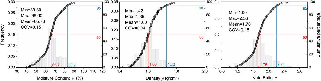
FIGURE 4. Histograms and cumulative distributions of the physical parameters ($\omega$, $\rho$, $e$) in CP tests.

TABLE 1

TABLE 1. Summary of the minimum, mean, median, maximum, and COV values for the physical ($\mathbf{\omega }$; $\mathbf{\rho }$, $\mathbf{e}$) and mechanical (${\mathbf{E}}_{\mathbf{s}}$; $\mathbf{\alpha }$) parameters taken from the database.

Figure 5 shows plots of the mechanical parameters ($E_s$and $\alpha$) versus the physical parameters ($\omega$, $\rho$, and $e$) in the CP tests. Visually, the mechanical parameters are statistically correlated to the physical parameters. For example, the modulus of compression $E_s$ tends to decrease as $\rho$ increases, and to increase as $\omega$ and $e$ increase. In contrast, for $\alpha$, the reverse trends occur, in which $\alpha$ decreases as $\omega$ and $e$ increase and increases as $\rho$ increases. The aforementioned correlations can be proved by Spearman’s rank correlation tests. As shown in Figure 5, all of the Spearman’s p-values for correlations between the physical and mechanical parameters were below 0.05.

FIGURE 5

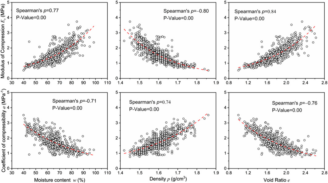
FIGURE 5. Plots of compression indices versus physical parameters in the CP test results.

It should be noted that various other factors, such as saturation, formation environment, stress history, liquid limit, plastic limit, and organic matter content, may also affect the compression indices of soft soils. Data on some of these are also available in the source database. For example, the degree of saturation was 100% for all soft soil samples. Moreover, all samples had similar formation environments and similar stress histories as they were taken from the same soil stratum. Hence, these two factors did not vary and were not explicitly considered here. Parameters such as liquid limit, plastic limit, and sampling depth were also excluded from the model input to keep the machine learning models simple, practical, and analytical.

4 Development and evaluation of ML models

This section first presents the details of the construction of machine learning models (i.e., the ANN, RF, and SVM models) for mapping to the compression indices of soft soils (i.e., $E_s$ and $\alpha$) from the physical parameters (i.e., $\omega$, $\rho$, and $e$) based on the database introduced in Section 3. Subsequently, an evaluation of the accuracy of each model is presented; these were evaluated on the basis of model biases $\lambda$ (i.e., ${\mathrm{\lambda }}_{E_s}$ and ${\mathrm{\lambda }}_{\mathrm{\alpha }}$), which are defined as the ratio of the measured to the predicted compression indices. Finally, the performances of the three models are compared.

4.1 Model construction

4.1.1 ANN model

The ANN configuration was determined using a trial-and-error approach, technical details of which are described by Lin et al. (2022). In this study, the use of one hidden layer containing three neurons was found to be adequate to yield satisfactorily accurate predictions while maintaining the simplicity of the network. It should be noted that, while the addition of more hidden layers and neurons can enhance the mapping ability of the ANN model, this did not produce a clear improvement in the present study and imposes a risk of overfitting due to an insufficiently large database (less than 10³ data points). Figure 6 illustrates the proposed ANN model for compression indices.

FIGURE 6

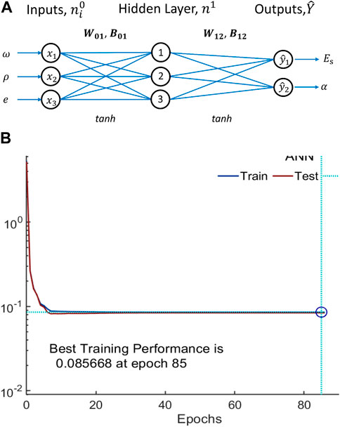
FIGURE 6. Plots of the training process for the ANN model: (A) illustration of the proposed ANN for mapping the compression indices of soft soils; (B) mean squared error (MSE) versus number of epochs during training of the ANN model.

As shown in Figure 6A, the tanh activation function was used in connections both from the input layer to the hidden layer and from the hidden layer to the output layer. The corresponding weight and bias matrices are ${\mathbf{W}}_{01}$ and ${\mathbf{B}}_{01}$ and ${\mathbf{W}}_{12}$ and ${\mathbf{B}}_{12}$, consisting of 3×3 elements in ${\mathbf{W}}_{01}$, 3×1 elements in ${\mathbf{B}}_{01}$, 2×3 elements in ${\mathbf{W}}_{12}$, and 2×1 elements in ${\mathbf{B}}_{12}$. Through comparison of the measured compression indices and the corresponding predictions, the squared error was calculated as ${\epsilon }_k^2={\left({\widehat{Y}}_{p,k}-Y_{m,k}\right)}^2$. Therefore, the mean squared error (MSE) ${\epsilon }^2={\displaystyle \sum _{k=1}^{k=743}}{\epsilon }_k^2/743$ was obtained by traversing all samples and calculating the mean of all squared errors. The MSE was used as the optimization indicator for training the ANN; this was therefore minimized to determine the optimal values of ${\mathbf{W}}_{01}$, ${\mathbf{W}}_{12}$, ${\mathbf{B}}_{01}$, and ${\mathbf{B}}_{12}$.

The ANN model was constructed, trained, and tested via the MATLAB™ platform using Bayesian regularization (BR) training algorithms. Since the built-in BR backpropagation algorithm in MATLAB™ simultaneously trains and verifies an ANN model, designation of an additional validation set was not necessary. Hence, the input matrix $\mathbf{I}=\left[\omega ,\rho ,e\right]$ was divided into two sub-matrices: a training set ${\mathbf{I}}_{train}$ (3×520) containing 70% of the data from $\mathbf{I}$, and a test set ${\mathbf{I}}_{test}$ (3×223) containing the remaining data. Similarly, the output matrix $\mathrm{Y}$ consisted of two subsets, ${\widehat{\mathbf{Y}}}_{train}$ and ${\widehat{\mathbf{Y}}}_{test}$, containing 70% and 30% of $\widehat{\mathbf{Y}}$, respectively. ${\mathbf{I}}_{train}$ and ${\widehat{\mathbf{Y}}}_{train}$ should match. Other percentages may be employed in dividing the data into training and test sets; however, the influence of this choice was insignificant in this case, due to the abundance of the available data to establish the ANN (Figure 6A).

As shown in Figure 6B, the MSE gradually reached a minimum value as the epoch increased. Here, an epoch is a complete training cycle in which all data are used once and the weights and biases are optimized to yield the minimum MSE. Training was stopped at epoch 85, at which point the best training performance (lowest MSE) was 0.085668. The optimal ${\mathbf{W}}_{01}$, ${\mathbf{W}}_{12}$, ${\mathbf{B}}_{01}$, and ${\mathbf{B}}_{12}$ were determined to be:

${\mathit{W}}_{\mathbf{01}}=\left[\begin{array}{l}0.3341.1910.520\\ -0.357-1.066-1.738\\ -0.4200.175-1.138\end{array}\right],{\mathbf{B}}_{\mathbf{01}}=\left[\begin{array}{l}0.683\\ -0.282\\ -0.802\end{array}\right],$

${\mathit{W}}_{\mathbf{02}}=\left[\begin{array}{l}-1.225-1.0430.393\\ 0.6880.3710.365\end{array}\right],{\mathbf{B}}_{\mathbf{12}}=\left[\begin{array}{l}0.359\\ -0.375\end{array}\right].$

This ANN is simple, having an explicitly analytical form consisting of simple physical parameters, and it offers convenience for engineers in that the model can readily be applied in practice. The technical details are described by Lin et al. (2022).

4.1.2 RF model

The RF model was also developed using the MATLAB™ platform. As discussed in Section 2.2, OOB error is used as an optimization indicator for RF models, and is determined by the numbers of trees (B) and leaves ($N_L$). Figure 7 shows the OOB MSEs (OOB errors) for both $E_s$ and $\alpha$ with $B=\left[\mathrm{1,50}\right]$ and $N_L=5$, 10, 20, 50, and 100. Visually, the OOB MSE decreased as $B$ increased, but became very stable after $B\ge 20$ in the case of both $E_s$ and $\alpha$. While increasing the $B$ value continuously reduced the OOB MSE, the reduction was insignificant in practical terms and a larger $B$ value could result in overfitting. Therefore, the number of trees used in this case was $B=20$ for both $E_s$ and $\alpha$. Regarding the number of leaves $N_L$, the OOB MSEs reached a minimum value of 0.095898 for $E_s$ for $N_L=10$, and a minimum value of 0.087289 for $\alpha$ for $N_L=20$. Furthermore, the number of features $m$ is routinely determined to be $m=\sqrt{p}$ or $m=p/3$ according to Efron and Hastie (2016). Hence, parameter $m$ was either 1 or 2. Based on this analysis, the parameters selected for the RF model developed to estimate each of the compression indices were $B=20$, $N_L=10$ for $E_s$ and $B=20$, $N_L=20$ for $\alpha$.

FIGURE 7

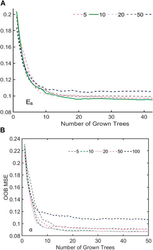
FIGURE 7. Influence of the number of trees and leaves on OOB MSE in the RF model: (A) for $E_s$; (B) for $\mathrm{\alpha }$.

4.1.3 SVM model

The key points in establishing an SVM regression model are to determine the kernel function and to optimize the model parameters. In this study, the main options considered for the kernel function were Gaussian, polynomial, sigmoid, and linear kernels. The corresponding MSEs for the SVM model using each of these kernels, based on the full dataset, were computed as 0.0840 for the Gaussian kernel, 0.1178 for the polynomial kernel, 0.0929 for the sigmoid kernel, and 0.0925 for the linear kernel. In addition, the corresponding coefficients of determination ($R^2$) were 0.6892, 0.5639, 0.6561, and 0.6577, respectively. These two indicators clearly showed that the Gaussian kernel function was the best option; this kernel represents a local smoothing fit, the value of which decreases as the distance between a data point and the hyperplane increases. The polynomial kernel was not selected since this type of kernel is computationally intensive and time-consuming. The sigmoid and linear kernels were not adopted here owing to low prediction accuracy compared to the Gaussian kernel. Therefore, the Gaussian kernel was used for development of the SVM model for prediction of compression indices.

Optimization of model parameters for this type of model mainly involves the penalty $C$ and the Gaussian kernel coefficient $\xi$. Typically, the larger the penalty, the higher the loss and the lower the number of support vectors; thus, the more complicated the hyperplane is. The coefficient $\xi$ reflects the influence of a single point on the hyperplane. A data point with a larger $\xi$ means selection of the support vector is more difficult. In this study, the setting ranges used for both $C$ and $\xi$ were [–10, 10], and the interval was 0.5, producing a matrix of settings $C\times \xi =41\times 41$ and a total of 1,681 combinations of $C$ and $\xi$. Using the same datasets to train and test the SVM model for each $\left[C,\xi \right]$ combination, values of $C=0$ and $\xi =-1.0$ were found to lead to the minimum MSE. Hence, these values were used in the SVM model for prediction of compression indices.

4.2 Model evaluation

The $R^2$ values calculated on the basis of all data were 0.827, 0.769, and 0.689 for the ANN, RF, and SVM models, respectively. While the MSE and $R^2$ values provided initial indications of the relative accuracies of the three models, bias statistics have practical use in further evaluating model uncertainties. In this study, bias statistics such as the mean and coefficient of variation (COV) were computed to further quantify the accuracy of the machine learning models developed. Here, bias is defined as the ratio of the measured to the predicted compression indices, i.e., ${\lambda }_{E_s}=E_{sm}/E_{sp}$ and ${\lambda }_{\alpha }={\alpha }_m/{\alpha }_p$. The means and COVs of the biases are summarized in Table 2. All the means were essentially 1.00 (range: 1.00 to 1.01), and the COVs were no greater than 0.20 (range: 0.15 to 0.17) across the ANN, RF, and SVM models. Therefore, the three models were accurate on average, and the prediction dispersion was low in all cases according to the ranking scheme proposed by Phoon and Tang (2019). Figure 8 shows plots of the measured versus predicted values for the ANN, RF, and SVM models. Visually, the data points are scattered around the line corresponding to Y=X for all three models. Most of the data fall within the range of 0.5–2, except for a few data points falling outside this range. This suggests that the performance of the three models was satisfactory. The bias statistics based on the aforementioned analyses for the three models were similar, with almost no difference in their performance. Therefore, it is difficult to judge the relative accuracy of the models based on the aforementioned analyses.

TABLE 2

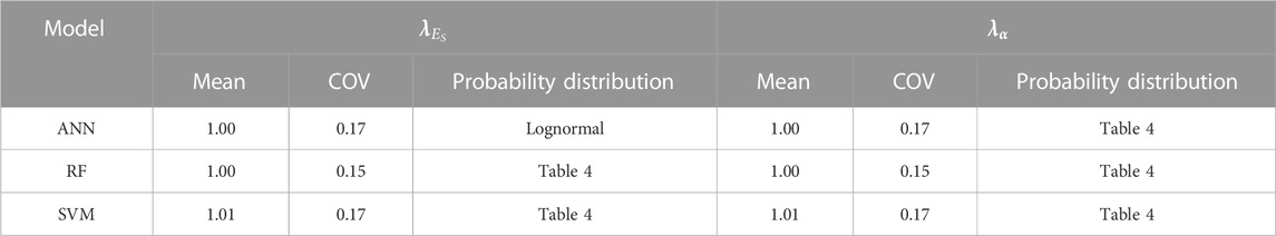
TABLE 2. Summary of the mean, COV, and probability distributions of the model biases for the ANN, RF, and SVM models.

FIGURE 8

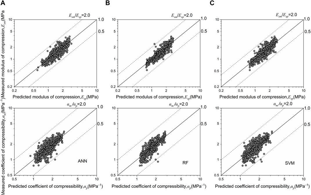
FIGURE 8. Measured compression indices versus values predicted by the trained ML models using all datasets: (A–C) $E_{sm}$ versus $E_{sp}$and ${\alpha }_m$ versus ${\alpha }_p$ for the ANN, RF, and SVM models, respectively.

Figure 9 shows the plots of $\lambda$ versus the predicted values for each model. Externally, no dependencies are observed between the biases and predicted values. Spearman’s rank correlation tests showed that the biases and predicted values were statistically uncorrelated at a significance level of 0.05 in the case of the ANN and SVM models, while a weak correlation was found in the case of the RF model. The results of a further correlation check of $\lambda$ against each input parameter are summarized in Table 3. The $\lambda$ values (${\lambda }_{E_s}$ and ${\lambda }_{\alpha }$) for the RF model were statistically correlated with $\rho$, and the $\lambda$ values (${\lambda }_{E_s}$; ${\lambda }_{\alpha }$) for the SVM model were statistically correlated with all input parameters, which is not conducive to engineering practice. Based on the above analyses, it can be concluded that the ANN can be considered to be the best model in this study.

FIGURE 9

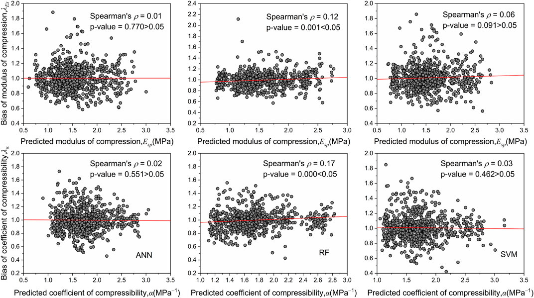
FIGURE 9. Plots of model biases versus predicted compression indices for the ANN, RF, and SVM models.

TABLE 3

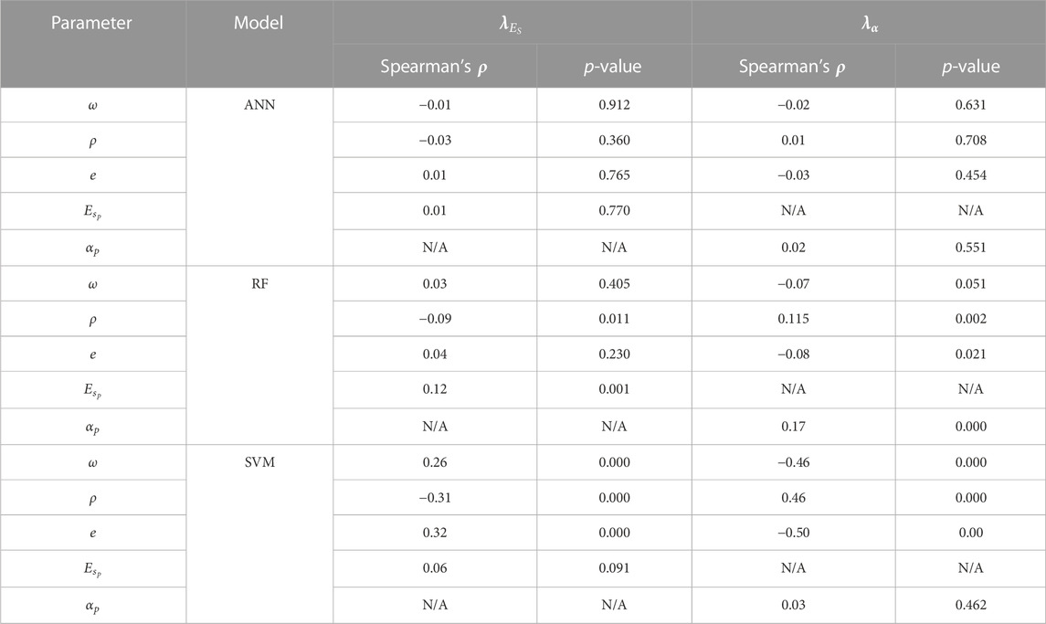
TABLE 3. Summary of results of Spearman’s rank correlation tests between biases and input parameters or predicted compressibility parameters.

5 Characterization of bias distributions

Aside from mean bias and bias COV, characterization of the probability distributions of variables is also common in geotechnical analysis (Guo et al., 2021). In this study, the probability distribution of the bias is an important input parameter in reliability-based geotechnical design; thus, this also required characterization. Figure 10 shows the cumulative distributions of all model biases. The Kolmogorov–Smirnov (K–S) normality test was applied to the logarithms of each model bias, i.e., ln ${\lambda }_{E_s}$ and ln ${\lambda }_{\alpha }$. The results showed that no p-values exceeded 0.05 except in the case of ln ${\lambda }_{E_s}$ in the ANN model (Figure 10). In other words, ${\lambda }_{E_s}$ for the ANN model can be treated as a lognormal random variable, while this is not the case for the remaining $\lambda$ distributions (five cases) across the three models. Additional goodness-of-fit tests, such as the K–S modified test and A-D test, were conducted to further examine the bias distributions; however, the results showed that none of the remaining model biases followed Weibull, gamma, or exponential distributions.

FIGURE 10

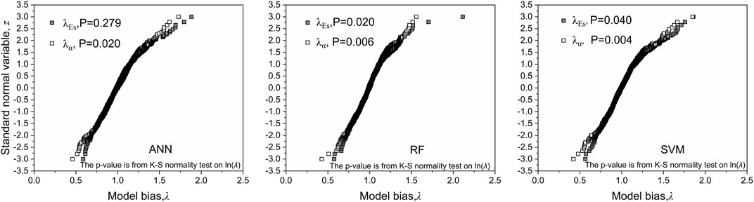
FIGURE 10. Cumulative distributions and K–S normality test results for the biases of the three ML models.

For the five cases that did not follow any common distribution, a fit-to-tail technique was used to linearly approximate the tail distribution of $\lambda$. Figure 11 plots the fit-to-tail fitted for the five sets of $\lambda$. These tail distributions of $\lambda$ can be treated as normal random variables. The mathematical expressions and bias statistics of the linear approximation curves and the corresponding coefficients of determination $R^2$ are summarized in Table 4. The overall probability distributions of $\lambda$ for all three models are also shown in Table 2.

FIGURE 11

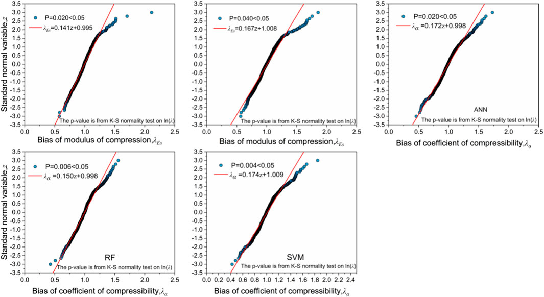
FIGURE 11. Fit-to-tail technique applied to the tail distributions of five model biases.

TABLE 4

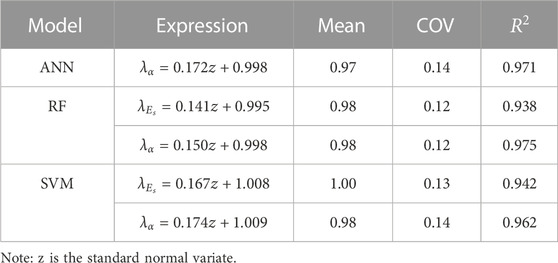
TABLE 4. Expressions and bias statistics for the ANN, RF, and SVM models using the fit-to-tail technique.

6 Conclusion

In this study, three machine learning techniques (i.e., an artificial neural network (ANN), a random forest (RF) model, and a support vector machine (SVM) model) were developed for mapping of the compression parameters of soft soils in the Greater Bay Area of China. The inputs were water content, soil density, and void ratio. The outputs were the modulus of compression and the coefficient of compressibility, which are usually obtained from laboratory consolidation tests. The accuracies of the three machine learning models developed were evaluated and compared using model bias statistics. The models were accurate on average, with low dispersion in prediction accuracy. The bias mean was essentially 1.00 in all cases, and the bias COVs were around 15%. The biases of each of the three models followed multi-order Gaussian distributions, with the exception of ${\lambda }_{E_s}$ in the ANN model, which followed a lognormal distribution. The ANN model was considered the best, as it was the only model in which the accuracies were not statistically correlated with the model inputs and output. The machine learning models developed in this study have practical value, as they can be easily used to efficiently predict the compressibility indices of soft soils in the Greater Bay Area of China. Moreover, these results demonstrate the value of applying ML-based mapping techniques to address geotechnical challenges.

Data availability statement

The raw data supporting the conclusion of this article will be made available by the authors, without undue reservation.

Author contributions

Conceptualization, HL and PL; methodology, PL; validation, JW; formal analysis, HL; investigation, HL and JW; writing—preparation of original draft, HL; writing—review and editing, PL; supervision, PL; funding acquisition, HL and PL.

Funding

This research was funded by the State Key Laboratory of Building Safety and Built Environment Open Foundation (grant no. BSBE 2021-03), the National Natural Science Foundation of China (52008408), the Guangdong Basic and Applied Basic Research Foundation (2021A1515012088), and the Science and Technology Program of Guangzhou, China (202102021017).

Conflict of interest

Author JW was employed by Guangdong Wisdom Cloud Engineering Science and Technology Co., Ltd.

The remaining authors declare that the research was conducted in the absence of any commercial or financial relationships that could be construed as a potential conflict of interest.

Publisher’s note

All claims expressed in this article are solely those of the authors and do not necessarily represent those of their affiliated organizations, or those of the publisher, the editors, and the reviewers. Any product that may be evaluated in this article, or claim that may be made by its manufacturer, is not guaranteed or endorsed by the publisher.

References

Acharyya, R. (2019). Finite element investigation and ANN-based prediction of the bearing capacity of strip footings resting on sloping ground. Int. J. Geo-Engineering 10 (5). 0100, doi:10.1186/s40703-019-0100-z

CrossRef Full Text | Google Scholar

Amiri, K. E., Emami, H., Mosaddeghi, M. R., and Astaraei, A. R. (2018). Estimation of unsaturated shear strength parameters using easily-available soil properties. Soil Tillage Res. 184, 118–127. doi:10.1016/j.still.2018.07.006

CrossRef Full Text | Google Scholar

Arditi, D., and Pulket, T. (2010). Predicting the outcome of construction litigation using an integrated artificial intelligence model. J. Comput. Civ. Eng. 24 (1), 73–80. doi:10.1061/(asce)0887-3801(2010)24:1(73)

CrossRef Full Text | Google Scholar

Bo, M. W., Lwin, T., and Choa, V. (2018). Application of specialized in-situ tests in changi east reclamation and ground improvement projects. Geotechnical Res. 6 (1), 1–50. doi:10.1680/jgere.18.00033

CrossRef Full Text | Google Scholar

Breiman, L. (2001). Random forests. Mach. Learn. 45 (1), 5–32. doi:10.1023/a:1010933404324

CrossRef Full Text | Google Scholar

Cao, Z., and Wang, Y. (2013). Bayesian approach for probabilistic site characterization using cone penetration tests. J. Geotechnical Geoenvironmental Eng. 139 (2), 267–276. doi:10.1061/(asce)gt.1943-5606.0000765

CrossRef Full Text | Google Scholar

Cao, Z-J., Zheng, S., Li, D-Q., and Phoon, K-K. (2019). Bayesian identification of soil stratigraphy based on soil behaviour type index. Can. Geotechnical J. 56 (4), 570–586. doi:10.1139/CGJ-2017-0714

CrossRef Full Text | Google Scholar

Çelik, S., and Tan, Ö. (2005). Determination of preconsolidation pressure with artificial neural network. Civ. Eng. Environ. Syst. 22 (4), 217–231. doi:10.1080/10286600500383923

CrossRef Full Text | Google Scholar

Chen, J., Vissinga, M., Shen, Y., Hu, S., Beal, E., and Newlin, J. (2021). Machine learning-based digital integration of geotechnical and ultrahigh-frequency geophysical data for offshore site characterizations. J. Geotechnical Geoenvironmental Eng. 147 (12), 04021160. doi:10.1061/(ASCE)GT.1943-5606.0002702

CrossRef Full Text | Google Scholar

Ching, J., and Phoon, K. K. (2014). Correlations among some clay parameters - the multivariate distribution. Can. Geotechnical J. 51 (6), 686–704. doi:10.1139/cgj-2013-0353

CrossRef Full Text | Google Scholar

Ching, J., and Schweckendiek, T. (2021) State-of-the-art review of inherent variability and uncertainty in geotechnical properties and models.ISSMGE Tech. Comm. 304, 56, doi:10.53243/R0001

CrossRef Full Text | Google Scholar

Das, S. K., Samui, P., Khan, S. Z., and Sivakugan, N. (2011). Machine learning techniques applied to prediction of residual strength of clay. Open Geosci. 3 (4), 449–461. doi:10.2478/s13533-011-0043-1

CrossRef Full Text | Google Scholar

Demuth Howard, B., Beale Mark, H., De Jess, O., and Hagan Martin, T. (2014). Neural network design. Boston, MA: PWS Publishing Co.

Google Scholar

Drucker, H., Burges Chris, J. C., Kaufman, L., Chris, J. C., Kaufman, B. L., Smola, A., et al. (1997). Support vector regression machines. Adv. Neural Inf. Process. Syst. 28 (7), 779–784.

Google Scholar

Efron, B., and Hastie, T. (2016). Computer age statistical inference 5. Cambridge, United Kingdom: Cambridge University Press.

Google Scholar

Goh, C. A. T., Wong, K. S., and Broms, B. B. (1995). Estimation of lateral wall movements in braced excavations using neural networks. Can. Geotechnical J. 32 (6), 1059–1064. doi:10.1139/t95-103

CrossRef Full Text | Google Scholar

Guo, C., Guo, P., Zhao, L., Lin, P., and Wang, F. (2021). A weibull-based damage model for shear softening behaviours of soil-structure interfaces. Geotechnical Res. 8 (4), 1–10. doi:10.1680/JGERE.20.00043

CrossRef Full Text | Google Scholar

Haykin, S. (2009). Neural networks and learning machines 3. Upper Saddle River: Pearson education.

Google Scholar

Holtz, R. D., Kovacs, W. D., and Sheahan, T. C. (2010). An introduction to geotechnical engineering. 2nd Ed. Upper Saddle River:NJ: PEARSON.

Google Scholar

Hou, Y., Li, Q., Zhang, C., Lu, G., Ye, Z., Chen, Y., et al. (2021). The state-of-the-art review on applications of intrusive Sensing,Image processing Techniques,and machine learning methods in pavement monitoring and analysis. Engineering 7 (6), 845–856. doi:10.1016/j.eng.2020.07.030

CrossRef Full Text | Google Scholar

Hu, H., and Lin, P. (2019). Analysis of resistance factors for LRFD of soil nail pullout limit state using default FHWA load and resistance models. Mar. Georesources Geotechnol. 38, 332–348. doi:10.1080/1064119x.2019.1571540

CrossRef Full Text | Google Scholar

Jin, Y., Giovanna, B., and Paolo, G. (2018). A bayesian definition of 'most probable' parameters. Geotechnical Res. 5 (3), 130–142. doi:10.1680/jgere.18.00027

CrossRef Full Text | Google Scholar

Kanungo, D. P., Sharma, S., and Pain, A. (2014). Artificial Neural Network (ANN) and Regression Tree (CART) applications for the indirect estimation of unsaturated soil shear strength parameters. Front. Earth Sci. 8 (3), 439–456. doi:10.1007/s11707-014-0416-0

CrossRef Full Text | Google Scholar

Kardani, N., Zhou, A., Nazem, M., and Shen, S-L. (2021). Improved prediction of slope stability using a hybrid stacking ensemble method based on finite element analysis and field data. J. Rock Mech. Geotechnical Eng. 13 (1), 188–201. doi:10.1016/j.jrmge.2020.05.011

CrossRef Full Text | Google Scholar

Kim, Y.-S., and Kim, B.-T. (2006). Use of artificial neural networks in the predictionof liquefaction resistance of sands. J. Geotechnical Geoenviron Ment. Eng. 132 (11), 1502–1504. doi:10.1061/(asce)1090-0241(2006)132:11(1502)

CrossRef Full Text | Google Scholar

Kiran, S., Lal, B., and Tripathy, S. (2016). Shear strength prediction of soil based on probabilistic neural network. Indian J. Sci. Technol. 9. 99188, doi:10.17485/ijst/2016/v9i41/99188

CrossRef Full Text | Google Scholar

Koppula, S. D. (1981). Statistical estimation of compression index. Geotechnical Test. J. 4 (2), 68. doi:10.1520/gtj10768j

CrossRef Full Text | Google Scholar

Krishnan, N. M. A., Mangalathu, S., Smedskjaer, M. M., Tandia, A., Burton, H., and Bauchy, M. (2018). Predicting the dissolution kinetics of silicate glasses using machine learning. J. Non-Crystalline Solids 487, 37–45. doi:10.1016/j.jnoncrysol.2018.02.023

CrossRef Full Text | Google Scholar

Liaw, A., and Wiener, M. (2002). Classification and regression by random Forest. R. news 2 (3), 18–22.

Google Scholar

Lim, Y. X., Tan, S. A., and Phoon, K-K. (2020). Friction angle and overconsolidation ratio of soft clays from cone penetration test. Eng. Geol. 274, 105730. doi:10.1016/j.enggeo.2020.105730

CrossRef Full Text | Google Scholar

Lin, P., Chen, X., Jiang, M., Song, X., Xu, M., and Huang, S. (2022). Mapping shear strength and compressibility of soft soils with artificial neural networks. Eng. Geol. 300, 106585. doi:10.1016/j.enggeo.2022.106585

CrossRef Full Text | Google Scholar

Liu, H., Liu, H., Xiao, Y., Chen, Q., Gao, Y., and Peng, J. (2018). Nonlinear elastic model incorporating temperature effects. Geotechnical Res. 5 (1), 22–30. doi:10.1680/jgere.17.00015

CrossRef Full Text | Google Scholar

Lunne, T., Berre, T., Andersen, K. H., Strandvik, S., and Sjursen, M. (2006). Effects of sample disturbance and consolidation procedures on measured shear strength of soft marine Norwegian clays. Can. Geotechnical J. 43 (7), 726–750. doi:10.1139/t06-040

CrossRef Full Text | Google Scholar

Makasis, N., Narsilio, G. A., and Bidarmaghz, A. (2018). A machine learning approach to energy pile design. Comput. Geotechnics 97, 189–203. doi:10.1016/j.compgeo.2018.01.011

CrossRef Full Text | Google Scholar

Mangalathu, S., and Jeon, J-S. (2018). Classification of failure mode and prediction of shear strength for reinforced concrete beam-column joints using machine learning techniques. Eng. Struct. 160, 85–94. doi:10.1016/j.engstruct.2018.01.008

CrossRef Full Text | Google Scholar

Mcgann, C. R., Bradley, B. A., Taylor, M. L., Wotherspoon, L. M., and Cubrinovski, M. (2015). Development of an empirical correlation for predicting shear wave velocity of Christchurch soils from cone penetration test data. Soil Dyn. Earthq. Eng. 75, 66–75. doi:10.1016/j.soildyn.2015.03.023

CrossRef Full Text | Google Scholar

Meng, J., Mattsson, H., and Laue, J. (2021). Three dimensional slope stability predictions using artificial neural networks. Int. J. Numer. Anal. Methods Geomechanics 45, 1988–2000. doi:10.1002/nag.3252

CrossRef Full Text | Google Scholar

Moayedi, H., Mosallanezhad, M., Asa, R., Jusoh, W., and Muazu, M. A. (2019). A systematic review and meta-analysis of artificial neural network application in geotechnical engineering: Theory and applications. Neural Comput. Appl. 32, 495–518. doi:10.1007/s00521-019-04109-9

CrossRef Full Text | Google Scholar

Motaghedi, H., and Eslami, A. (2014). Analytical approach for determination of soil shear strength parameters from CPT and CPTu data. Arabian J. Sci. Eng. 39 (6), 4363–4376. doi:10.1007/s13369-014-1022-x

CrossRef Full Text | Google Scholar

Müller, K. R., Smola, A. J., Bf, G. R., Schlkopf, B., and Vapnik, V. (1997). “Predicting time series with support vector machines,” in Proceedings of the 7th International Conference on Artificial Neural Networks, Berlin, Heidelberg, October 8 - 10, 1997.

Google Scholar

Naghibi, S. A., Ahmadi, S., and Daneshi, A. (2017) Application of support vector machine, random forest, and genetic algorithm optimized random forest models in groundwater potential mapping. WATER Resour. MANAG., 31(9): 2761–2775. doi:10.1007/s11269-017-1660-3

CrossRef Full Text | Google Scholar

Najjar, Y. M., and Huang, C. (2007). Simulating the stress–strain behavior of Georgia kaolin via recurrent neuronet approach. Comput. Geotechnics 34 (5), 346–361. doi:10.1016/j.compgeo.2007.06.006

CrossRef Full Text | Google Scholar

Orense, R. P., Mirjafari, Y., and Suemasa, N. (2018). Screw driving sounding: A new test for field characterisation. Geotechnical Res. 6 (1), 28–38. doi:10.1680/jgere.18.00024

CrossRef Full Text | Google Scholar

Pan, Q., and Dias, D. (2017). An efficient reliability method combining adaptive Support Vector Machine and Monte Carlo Simulation. Struct. Saf. 67, 85–95. doi:10.1016/j.strusafe.2017.04.006

CrossRef Full Text | Google Scholar

Park, H. I., and Lee, S. L. (2011). Evaluation of the compression index of soils using an artificial neural network. Comput. Geotechnics 38 (4), 472–481. doi:10.1016/j.compgeo.2011.02.011

CrossRef Full Text | Google Scholar

Pham, B. T., Nguyen, M. D., Ly, H. B., Pham, T. A., and Bui, G. L. (2019a). “Development of artificial neural networks for prediction of compression coefficient of soft soil,” in CIGOS 2019, innovation for sustainable infrastructure. Editors C. Ha-Minh, D. Dao, F. Benboudjema, S. Derrible, D. Huynh, and A. Tang (Singapore: Lecture Notes in Civil Engineering).

CrossRef Full Text | Google Scholar

Pham, B. T., Nguyen, M. D., Dao, D. V., Prakash, I., Ly, H-B., Le, T-T., et al. (2019b). Development of artificial intelligence models for the prediction of Compression Coefficient of soil: An application of Monte Carlo sensitivity analysis. Sci. Total Environ. 679, 172–184. doi:10.1016/j.scitotenv.2019.05.061

PubMed Abstract | CrossRef Full Text | Google Scholar

Pham, B. T., Son, L. H., Hoang Tuan, A, Manh, N. D., and Dieu, T. B. (2018). Prediction of shear strength of soft soil using machine learning methods. Catena 166, 181–191. doi:10.1016/j.catena.2018.04.004

CrossRef Full Text | Google Scholar

Phoon, K-K., and Kulhawy, F. H. (1999). Characterization of geotechnical variability. Can. Geotechnical J. 36 (4), 612–624. doi:10.1139/t99-038

CrossRef Full Text | Google Scholar

Phoon, K-K., and Tang, C. (2019).Characterisation of geotechnical model uncertainty, Georisk: Assess. Manag. Risk Eng. Syst. Geohazards, 13, 101–130. doi:10.1080/17499518.2019.1585545

CrossRef Full Text | Google Scholar

Rafiq, M. Y., Bugmann, G., and Easterbrook, D. J. (2001). Neural network design for engineering applications. Comput. Struct. 79 (17), 1541–1552. doi:10.1016/s0045-7949(01)00039-6

CrossRef Full Text | Google Scholar

Sadegh, E. M., Abbaspour, M., Abbasianjahromi, H., and Mariani, S. (2021). Machine learning-based prediction of the seismic bearing capacity of a shallow strip footing over a void in heterogeneous soils. Algorithms 14 (10), 288. doi:10.3390/a14100288

CrossRef Full Text | Google Scholar

Samui, P., Sitharam, T. G., and Kurup, P. U. (2008). OCR prediction using support vector machine based on piezocone data. J. Geotechnical Geoenvironmental Eng. 134: 894–898. doi:10.1061/(asce)1090-0241(2008)134:6(894

CrossRef Full Text | Google Scholar

Schneider, J. A., Randolph, M. F., Mayne, P. W., and Ramsey, N. R. (2008). Analysis of factors influencing soil classification using normalized piezocone tip resistance and pore pressure parameters. J. Geotechnical Geoenvironmental Eng. 134 (11), 1569–1586. doi:10.1061/(asce)1090-0241(2008)134:11(1569)(ASCE)1090-0241

CrossRef Full Text | Google Scholar

Scholkopf, B., and Smola, A. J. (2018). Learning with kernels: Support vector machines, regularization, optimization, and beyond: Adaptive computation and machine learning series. Massachusetts, United States: The Mit Press.

Google Scholar

Scholkopf, B., Sung, K-K., Burges, C. J. C., Girosi, F., Niyogi, P., Poggio, T., et al. (1997). Comparing support vector machines with Gaussian kernels to radial basis function classifiers. IEEE Trans. Signal Process. 45 (11), 2758–2765. doi:10.1109/78.650102

CrossRef Full Text | Google Scholar

Shahin Mohamed, A. (2016). State-of-the-art review of some artificial intelligence applications in pile foundations. Geosci. Front. 7 (1), 33–44. doi:10.1016/j.gsf.2014.10.002

CrossRef Full Text | Google Scholar

Smola, A. J., and Schölkopf, B. (2004). A tutorial on support vector regression. Statistics Comput. 14 (3), 199–222. doi:10.1023/b:stco.0000035301.49549.88

CrossRef Full Text | Google Scholar

Wang, B., Hou, H., and Zhu, Z. (2021). Transparency and applications of transparentsoil: A review. Geotechnical Res. 8, 130–138. doi:10.1680/jgere.21.00016

CrossRef Full Text | Google Scholar

Yan, W. M., Yuen, K-V., and Yoon, G. L. (2009). Bayesian probabilistic approach for the correlations of compression index for marine clays. J. Geotechnical Geoenvironmental Eng. 135 (12), 1932–1940. doi:10.1061/(ASCE)GT.1943-5606.0000157

CrossRef Full Text | Google Scholar

Yoon, G. L., Kim, B. T., and Jeon, S. S. (2004). Empirical correlations of compression index for marine clay from regression analysis. Can. Geotechnical J. 41 (6), 1213–1221. doi:10.1139/t04-057

CrossRef Full Text | Google Scholar

Zabielska, -A., and Katarzyna, S. (2018). One-dimensional compression and swelling of compacted fly ash. Geotechnical Res. 5 (2), 96–105. doi:10.1680/jgere.17.00017

CrossRef Full Text | Google Scholar

Zhang, D. M., Zhang, J. Z., Huang, H. W., Qi, C. C., and Chang, C. Y. (2020a). Machine learning-based prediction of soil compression modulus with application of 1D settlement. J. Zhejiang University-SCIENCE A 21 (6), 430–444. doi:10.1631/jzus.a1900515

CrossRef Full Text | Google Scholar

Zhang, J., Hu, J., Li, X., and Li, J. (2020b). Bayesian network based machine learning for design of pile foundations. Automation Constr. 118, 103295. doi:10.1016/j.autcon.2020.103295

CrossRef Full Text | Google Scholar

Zhang, L., Shi, B., Zhu, H., Yu, X. B., Han, H., and Fan, X. (2021). PSO-SVM-based deep displacement prediction of Majiagou landslide considering the deformation hysteresis effect. Landslides 18 (1), 179–193. doi:10.1007/s10346-020-01426-2

CrossRef Full Text | Google Scholar

Zhang, L., Shi, B., Zhu, H., Yu, X., and Wei, G. (2020c). A machine learning method for inclinometer lateral deflection calculation based on distributed strain sensing technology. Bull. Eng. Geol. Environ. 79 (7), 3383–3401. doi:10.1007/s10064-020-01749-3

CrossRef Full Text | Google Scholar

Zhang, R., Wu, C., Goh, A. T. C., and Wang, L. (2020d). Assessment of basal heave stability for braced excavations in anisotropic clay using extreme gradient boosting and random forest regression. Undergr. Space 7, 233–241. doi:10.1016/j.undsp.2020.03.001

CrossRef Full Text | Google Scholar

Zhang, W., Li, Y., Wu, C., Li, H., Goh, A. T. C., and Liu, H. (2020f). Prediction of lining response for twin tunnels constructed in anisotropic clay using machine learning techniques. Undergr. Space 6, 353–363. doi:10.1016/j.undsp.2020.02.007

CrossRef Full Text | Google Scholar

Zhang, W., Wu, C., Zhong, H., Li, Y., and Wang, L. (2021). Prediction of undrained shear strength using extreme gradient boosting and random forest based on Bayesian optimization. Geosci. Front. 12 (01), 469–477. doi:10.1016/j.gsf.2020.03.007

CrossRef Full Text | Google Scholar

Zhang, W., Xiao, R., Shi, B., Zhu, H., and Sun, Y. (2019). Forecasting slope deformation field using correlated grey model updated with time correction factor and background value optimization. Eng. Geol. 260, 105215. doi:10.1016/j.enggeo.2019.105215

CrossRef Full Text | Google Scholar

Zhang, W., Zhang, R., Wu, C., Goh, A. T. C., Lacasse, S., Liu, Z., et al. (2020e). State-of-the-art review of soft computing applications in underground excavations. Geosci. Front. 11 (4), 1095–1106. doi:10.1016/j.gsf.2019.12.003

CrossRef Full Text | Google Scholar

Zhang, W., and Ching, J. (2021). Big data and machine learning in geoscience and geoengineering: Introduction. Geosci. Front., 12, 327–329. doi:10.1016/j.gsf.2020.05.006

CrossRef Full Text | Google Scholar

Zhang, W., Li, H. R., Wu, C. Z., Li, Y. Q., Liu, Z. Q., and Liu, H. L. (2020g). Soft computing approach for prediction of surface settlement induced by Earth pressure balance shield tunneling. Undergr. Space 6, 353–363. doi:10.1016/j.undsp.2019.12.003

CrossRef Full Text | Google Scholar