A practical analytical model for performance prediction in unconventional gas reservoir

Ninety percentage of newly proven natural gas reservoirs of China are mainly unconventional resources, which can be typically developed by multi-stage fracturing horizontal well technology. Two regions typically occur near each fracture after hydraulic fracturing, in which the lower permeability region is considered as the storage source and the higher permeability region as the flow channel. The existed analytical models so far are mainly derived by Laplace transforming. In this paper, an improved practical analytical solution is derived for unconventional gas reservoirs bypassing the Laplace transform and numerical inversion. Through solving material balance equation and adopting the integration, a rate vs. pseudo-time solution in real-time domain can be directly obtained. Five numerical cases are created to verify the accuracy of the proposed analytical solution and the ratio of regular/irregular region pore volume is also proved to be derived reversely by the output parameters, which is significant for the field engineers to evaluate the effect of hydraulic fracturing. Moreover, a field example of a multi-fractured horizontal well in a tight gas reservoir is provided for demonstrate application.

1 Introduction

Unconventional resources including tight gas and shale gas have become a significant source of global hydrocarbon supply due to advanced reservoir evaluation and drilling/completion/fracturing technology (Clarkson, 2013; Dejam et al., 2018). As for the ultra-low permeability in unconventional reservoirs, the volume fracturing technology is adopted extensively to improve reservoir properties and achieve economic exploitation. Due to the dense distribution of the pre-existing natural fractures, the complex fracture geometry with high permeability will be created around the hydraulic fractures after fracturing operation (Wei et al., 2019; Xia et al., 2019; Liu et al., 2021), which is significant for fluid flow and resource extraction.

In order to make accurate reservoir evaluation, a large number of studies have been conducted for production data analysis. The popular techniques for quantitative production data analysis including empirical methods, numerical methods and analytical models. Firstly, the typical empirical methods, firstly proposed by Arps (1945), have been evolved by many researchers (Fetkovich, 1980; Blasingame et al., 1991; Duong, 2011). These decline curve analysis methods remain commonly used because of their simple and fast empirical regression. However, these methods will result in significant errors especially when applied to unconventional reservoirs. Numerical simulation for unconventional reservoirs has received extensive attention (Cipolla et al., 2010; Ding et al., 2014; Rao et al., 2022). However, it is a time-consuming process and depends on numerous original physical parameters. Compared with the numerical simulation, the analytical methods are models that derive analytically solutions to mathematical models including reservoir behavior as well as flow behavior associated with complex fracture geometry. Therefore, many scholars have focused on analytical models for production data analysis in unconventional reservoirs. Ci-qun (1983) proposed the analytical solution considering the two-dimensional pseudo steady state flow from two matrix blocks to the fracture. Lee and Brockenbrough, (1983) derived a tri-linear model to represent the transient flow behavior within the single fracture in an infinite homogeneous reservoir. Wattenbarger et al. (1998) represented an analytical solution accounting for linear flow in fractures with infinite conductivity applied in tight gas wells. Brown et al. (2011) presented a three-region analytical model considering the hydraulic fracture region, the stimulated region including dense branch fractures as well as the outer region containing low permeability matrix beyond the tip of hydraulic fractures. Stalgorova and Mattar, (2012) also introduced a three-region analytical model to consider complex fracture geometry. The outer region in their model adjacent to the stimulated region, which is the only difference from Brown et al. (2011) model. Stalgorova and Mattar, (2013) extended the three-region model to five-region model. Three outer regions are considered in their model. And it notes that the contribution from the outer regions may be negligible except for very late in the production life of the well. Abbassi et al. (2019) put forward a three-region model considering the transient flow among matrix, vugs and fractures. The analytical relationship for calculating the shape factor between different regions is also presented.

The analytical solutions mentioned above were derived analytically based on Laplace-transform technique and the final solution in real-time domain can be obtained by Stehfest numerical inversion (Stehfest, 1970). Development of a straightforward solution for analytical model considering the complex fracture geometry is still lacking. Ogunyomi et al. (2016) and Qiu andLi, (2018) presented the approximate analytical solutions to the dual-porosity model and triple-porosity model in real-time domain separately by adopting the integration and average pressure replacement. However, their solutions are applicable for tight oil reservoirs because the pressure-dependent properties in their model are not taken into consideration.

In this paper, our goal is to derive a straightforward solution in real-time domain for unconventional gas reservoirs considering complex fractures. Firstly, we define two regions and the high permeability regions contains hydraulic fractures and complex branch fractures as well as the low permeability region which adjacent to the high permeability region contains the matrix. Then the pseudo-variables (Anderson and Mattar, 2005) are introduced to eliminate the non-linearity caused by the pressure-dependent properties of gas. The derivation is based on the integration in real-time domain bypassing Laplace transform and numerical inversion. Lastly, the accuracy of the analytical solution is validated with equivalent numerical model.

2 Model description

In order to improve gas production in unconventional reservoirs, it is necessary to create as much connection between the unconventional gas reservoir and artificial or natural fractures as possible. Therefore, multistage hydraulic fracturing technology is applied to generate the hydraulic fractures and complex fracture networks to improve gas recovery. As shown in Figure 1A, there is a network of branch fractures forming the flow channel within the tight matrix. By virtue of the highly connected and high conductivity of the network of fractures, the oil/gas stored in ultra-tight matrix can flow into the wellbore. The black arrows represent the flow directions. Obviously, the flow in fractures network is complex and it is impossible to describe each flow process using mathematical models. Therefore, we simplified the complex flow system into two-region system, in which the defined high permeability region (Region 1) includes all the fractures and the low permeability region (Region 2) is the aggregated volume of the matrix directly connected to the high permeability region. Because the contribution of regions beyond hydraulic fractures is validated to be negligible after comparing the results of numerical simulation with and without region beyond fractures (Stalgorova and Mattar, 2012; Abbassi et al., 2019). Figure 1B is a 3D schematic of the reservoir with a multi-stage horizontal well, which is the conceptual model for constructing analytical model.

FIGURE 1

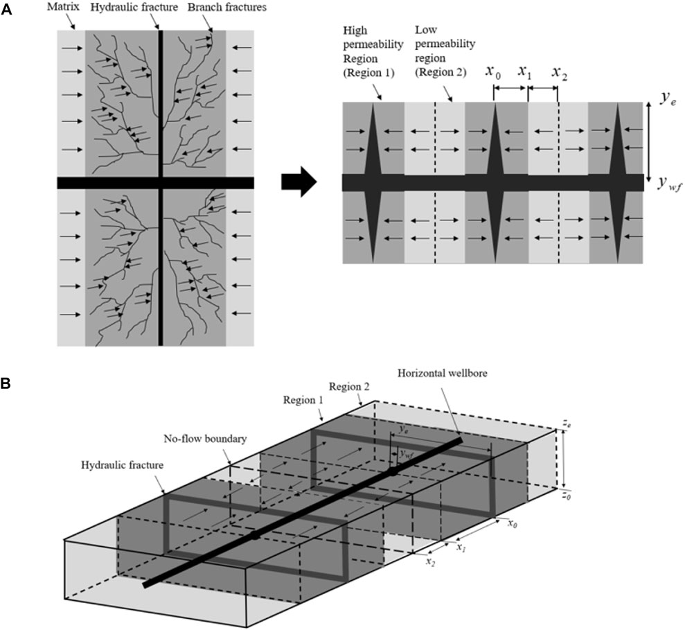
FIGURE 1. Schematic of a multi-stage fractured horizontal well with complex fractures. (A) The complex fractures after hydraulic fracturing. (B) 3D schematic of a multi-stage fractured horizontal well with two-regions around the hydraulic fractures.

In this paper, our analytical model is derived analytically based on the following assumption.

1. The reservoir is homogeneous, and isothermal.

2. Flow process is linear in each region.

3. Flow is single gas phase.

4. Flow within the hydraulic fracture is neglected for the high-speed gas flow rate.

5. Flow process is under constant bottom-hole pressure.

6. Pressure at the interface between two regions is constant.

7. Gravity effect is neglected.

Once the gas flow reaches the boundary and reservoir average pressure will decrease, and meanwhile the gas properties such as gas viscosity (μ), gas compressibility (C_t) and gas compressibility (Z) is varying with reservoir pressure. Consequently, the gas diffusivity equation will be non-linear which is impossible to derive the analytical solution directly. In order to deal with this problem, the pseudo-pressure and pseudo-time (Anderson and Mattar, 2005) are adopted to linearize the equation. The equations for pseudo-pressure and pseudo-time can be expressed as,

$m\left(p\right)=2\underset{0}{\overset{p}{{\displaystyle \int }}}\frac{p}{\mu z}dp(1)$

$t_a=\underset{0}{\overset{t}{{\displaystyle \int }}}\frac{{\left(\mu C_t\right)}_i}{\mu \left(\overline{p}\right)C_t\left(\overline{p}\right)}dt(2)$

3 Model development

The system of equations based on the conceptual model is presented below. In the low-permeability region (Region 2), the governing equation for gas flow after substituting the Eqs 1, 2 is expressed as:

$\frac{{\partial }^2{m}_2\left(p\right)}{\partial x^2}+\frac{{\partial }^2{m}_2\left(p\right)}{\partial y^2}+\frac{{\partial }^2{m}_2\left(p\right)}{\partial z^2}=\frac{{\left(\varphi \mu C_t\right)}_2}{k_2}\frac{\partial m_2\left(p\right)}{t_a}(3)$

Where m₂(p) is the pseudo-pressure in region 2, x, y and z are Cartesian coordinates, t_a is the pseudo-time for gas flow, k₂ and Φ is the permeability and porosity, respectively, of region 2.

The initial condition for the region 2 is equal to initial reservoir pseudo-pressure before the production start.

$m_2\left(p\right)\left(x,y,z,0\right)=m\left(p_i\right)(4)$

Where m (p_i) is the initial reservoir pseudo-pressure.

The closed boundary is defined for the top and bottom of the reservoir. Therefore, the outer boundary conditions are regarded as no-flow boundaries.

${\left.\frac{\partial m_2\left(p\right)}{\partial y}\right|}_{y=y_{wf},y_e}=0(5)$

${\left.\frac{\partial m_2\left(p\right)}{\partial z}\right|}_{z=z_0,z_e}=0(6)$

Considering the symmetry between adjacent hydraulic fractures, the location of x = x₂ is also regarded as no-flow boundary.

${\left.\frac{\partial m_2\left(p\right)}{\partial x}\right|}_{x=x_2}=0(7)$

Continuity of the flux and pressure across the boundaries between two regions is assumed. Therefore, the inner boundary condition can be written as,

${\left.\frac{k_2}{\mu }\frac{\partial m_2\left(p\right)}{\partial x}\right|}_{x=x_1}{\left.=\frac{k_1}{\mu }\frac{\partial m_1\left(p\right)}{\partial x}\right|}_{x=x_1}(8)$

Similarly, the governing equation for gas flow in region 1 can be also expressed as,

$\frac{{\partial }^2{m}_1\left(p\right)}{\partial x^2}+\frac{{\partial }^2{m}_1\left(p\right)}{\partial y^2}+\frac{{\partial }^2{m}_1\left(p\right)}{\partial z^2}=\frac{{\left(\varphi \mu C_t\right)}_1}{k_1}\frac{\partial m_1\left(p\right)}{t_a}(9)$

Where m₁(p) is the pseudo-pressure in region 1, x, y and z are Cartesian coordinates, t_a is the pseudo-time for gas flow, k₁ and Φ is the permeability and porosity in region 1 respectively.

In regard to the whole flow process, the initial condition of two regions is identical. And the constant bottom-hole pressure is assumed. Thus, the pressure is equal to the bottom-hole pressure at the location of x = x₀.

$m_1\left(p\right)\left(x,y,z,0\right)=m\left(p_i\right)(10)$

$m_1\left(p\right)\left(x=x_0,y,z,t_a\right)=m\left(p_{wf}\right)(11)$

Where m (p_wf) is the bottom-hole pseudo-pressure.

The flow in two regions is both 1D linear flow in the x-direction. Therefore, the outer boundary conditions are identical to those of region 2.

${\left.\frac{\partial m_1\left(p\right)}{\partial y}\right|}_{y=y_{wf},y_e}=0(12)$

${\left.\frac{\partial m_1\left(p\right)}{\partial z}\right|}_{z=z_0,z_e}=0(13)$

The inner boundary condition based on the continuity of flux at the location of x=x₁ is expressed as:

${\left.\frac{k_1}{\mu }\frac{\partial m_1\left(p\right)}{\partial x}\right|}_{x=x_1}={\left.\frac{k_2}{\mu }\frac{\partial m_2\left(p\right)}{\partial x}\right|}_{x=x_1}(14)$

4 Analytical solution

The equations mentioned above used for mathematical model are partial differential equations (PDEs). To solve mathematical model analytically, the system of PDEs must be transformed into the system of ordinary differential equations (ODEs). Considering the Laplace transform and numerical inversion are time-consuming, the integration method is adopted in this paper to eliminate the spatial dependences and obtain the ODEs directly. Integrating the governing equation with respect to spatial coordinates for region 2:

$\underset{x_1}{\overset{x_2}{{\displaystyle \int }}}\underset{y_{wf}}{\overset{y_e}{{\displaystyle \int }}}\underset{z_o}{\overset{z_e}{{\displaystyle \int }}}\frac{\partial }{\partial x}\left(\frac{\partial m_2\left(p\right)}{\partial x}\right)dxdydz+\underset{x_1}{\overset{x_2}{{\displaystyle \int }}}\underset{y_{wf}}{\overset{y_e}{{\displaystyle \int }}}\underset{z_o}{\overset{z_e}{{\displaystyle \int }}}\frac{\partial }{\partial y}\left(\frac{\partial m_2\left(p\right)}{\partial y}\right)dxdydz+\underset{x_1}{\overset{x_2}{{\displaystyle \int }}}\underset{y_{wf}}{\overset{y_e}{{\displaystyle \int }}}\underset{z_o}{\overset{z_e}{{\displaystyle \int }}}\frac{\partial }{\partial z}\left(\frac{\partial m_2\left(p\right)}{\partial z}\right)dxdydz=\frac{{\left(\varphi \mu C_t\right)}_2}{k_2}\frac{\partial }{\partial t_a}\underset{x_1}{\overset{x_2}{{\displaystyle \int }}}\underset{y_{wf}}{\overset{y_e}{{\displaystyle \int }}}\underset{z_o}{\overset{z_e}{{\displaystyle \int }}}{m}_2\left(p\right)dxdydz(15)$

The pseudo-time can be moved outside the spatial integral because the pseudo-time is independent of the spatial coordinates. To obtain a simplified equation, we define the average pseudo-pressure and the effective pore volume as:

$\overline{m}\left(p\right)=\frac{\iiint m\left(p\right)}{\iiint dxdydz}=\frac{\iiint m\left(p\right)}{V_b}(16)$

$V_p=\varphi V_b(17)$

Where V_b is the volume of the region and V_p is the pore volume of the region.

Substituting the Eqs 15–17 can be rewritten as:

$\underset{y_{wf}}{\overset{y_e}{{\displaystyle \int }}}\underset{z_0}{\overset{z_e}{{\displaystyle \int }}}\left({\left.\frac{\partial m_2\left(p\right)}{\partial x}\right|}_{x_2}-{\left.\frac{\partial m_2\left(p\right)}{\partial x}\right|}_{x_1}\right)dydz+\underset{x_1}{\overset{x_2}{{\displaystyle \int }}}\underset{z_0}{\overset{z_e}{{\displaystyle \int }}}\left({\left.\frac{\partial m_2\left(p\right)}{\partial y}\right|}_{y_e}-{\left.\frac{\partial m_2\left(p\right)}{\partial y}\right|}_{y_{wf}}\right)dxdz+\underset{x_1}{\overset{x_2}{{\displaystyle \int }}}\underset{y_{wf}}{\overset{y_e}{{\displaystyle \int }}}\left({\left.\frac{\partial m_2\left(p\right)}{\partial z}\right|}_{z_e}-{\left.\frac{\partial m_2\left(p\right)}{\partial y}\right|}_{z_0}\right)dxdy=\frac{{\left(\varphi \mu C_t\right)}_2{V}_{b_2}}{k_2}\frac{d{\overline{m}}_2\left(p\right)}{d{t}_a}(18)$

With the use of the initial and boundary conditions, Eq. 18 can be simplified as:

$-\underset{y_{wf}}{\overset{y_e}{{\displaystyle \int }}}\underset{z_0}{\overset{z_e}{{\displaystyle \int }}}\left({\left.\frac{k_2}{\mu }\frac{\partial m_2\left(p\right)}{\partial y}\right|}_{x_1}\right)dydz={\left(V_{p_2}{C}_t\right)}_2\frac{d{\overline{m}}_2\left(p\right)}{d{t}_a}(19)$

According to the Darcy’s law, the following applies:

$q_2=\underset{y_{wf}}{\overset{y_e}{{\displaystyle \int }}}\underset{z_0}{\overset{z_e}{{\displaystyle \int }}}{\left.\frac{k_2}{\mu }\frac{\partial m_2\left(p\right)}{\partial y}\right|}_{x_1}dydz(20)$

Therefore, Eq. 19 can be rewritten as:

${\left(V_{p_2}{C}_t\right)}_2\frac{d\overline{m}\left(p\right)}{d{t}_a}=-q_2(21)$

Where V_p2 is the pore volume of region 2 and q₂ is the flow rate in region 2.

In region 1, we also apply the integration method to address the diffusion equation as:

$\underset{y_{wf}}{\overset{y_e}{{\displaystyle \int }}}\underset{z_0}{\overset{z_e}{{\displaystyle \int }}}\left({\left.\frac{\partial m_1\left(p\right)}{\partial x}\right|}_{x_1}-{\left.\frac{\partial m_1\left(p\right)}{\partial x}\right|}_{x_0}\right)dydz+\underset{x_0}{\overset{x_1}{{\displaystyle \int }}}\underset{z_0}{\overset{z_e}{{\displaystyle \int }}}\left({\left.\frac{\partial m_1\left(p\right)}{\partial y}\right|}_{y_e}-{\left.\frac{\partial m_1\left(p\right)}{\partial y}\right|}_{y_{wf}}\right)dxdz+\underset{x_0}{\overset{x_1}{{\displaystyle \int }}}\underset{y_0}{\overset{y_1}{{\displaystyle \int }}}\left({\left.\frac{\partial m_1\left(p\right)}{\partial z}\right|}_{z_e}-{\left.\frac{\partial m_1\left(p\right)}{\partial y}\right|}_{z_0}\right)dxdy=\frac{{\left(\varphi \mu C_t\right)}_1{V}_{b_1}}{k_1}\frac{d{\overline{m}}_1\left(p\right)}{d{t}_a}(22)$

After applying the initial and boundary conditions, Eq. 22 can be rewritten as,

$-\underset{y_{wf}}{\overset{y_e}{{\displaystyle \int }}}\underset{z_0}{\overset{z_e}{{\displaystyle \int }}}\left(\frac{k_1}{\mu }{\left.\frac{\partial m_1\left(p\right)}{\partial x}\right|}_{x_1}-\frac{k_1}{\mu }{\left.\frac{\partial m_1\left(p\right)}{\partial x}\right|}_{x_0}\right)dydz={\left(V_{p_1}{C}_t\right)}_1\frac{d{\overline{m}}_1\left(p\right)}{d{t}_a}(23)$

Note that the following applies:

$q_1=\underset{y_0}{\overset{y_1}{{\displaystyle \int }}}\underset{z_0}{\overset{z_e}{{\displaystyle \int }}}\left(\frac{k_1}{\mu }{\left.\frac{\partial m_1\left(p\right)}{\partial x}\right|}_{x_0}\right)dydz(24)$

Substituting Eqs 9, 16, 34, 38 into Eq. 24 results in:

${\left(V_{p_1}{C}_t\right)}_1\frac{d{\overline{m}}_1\left(p\right)}{d{t}_a}=-q_1+q_2(25)$

Where V_p1 is the pore volume of region 1, q₁ is the flow rate in region 1.

Obviously, the next step involves the substitution of the average pseudo-pressure with the relationship between the pressure and flow rate. Since it is assumed that gas flows sequentially from region 2 into region 1, a general analytical solution for 1D linear gas flow is derived to solve the problem (Details are provided in Supplementary Appendix SA), which is given by:

$\overline{m}\left(p\right)=m\left(p_{wf}\right)+\frac{4}{{\pi }^2}\left[m\left(p_i\right)-m\left(p_{wf}\right)\right]{\displaystyle \sum }_{n=1}^{\infty }\frac{q_{D_n}}{{\left(2n-1\right)}^2}(26)$

Where $\overline{m}\left(p\right)$ is the average pseudo-pressure, $q_{Dn}$ is the dimensionless production of the nth mode.

Based on the model assumptions, the average pseudo-pressure in each region can be expressed as:

${\overline{m}}_1\left(p\right)=m\left(p_{wf}\right)+\frac{4}{{\pi }^2}\left[m\left(p_i\right)-m\left(p_{wf}\right)\right]{\displaystyle \sum }_{n=1}^{\infty }\frac{q_{D{1}_n}}{{\left(2n-1\right)}^2}(27)$

${\overline{m}}_2\left(p\right)={\overline{m}}_1\left(p\right)+\frac{4}{{\pi }^2}\left[m\left(p_i\right)-{\overline{m}}_1\left(p\right)\right]{\displaystyle \sum }_{n=1}^{\infty }\frac{q_{D{2}_n}}{{\left(2n-1\right)}^2}(28)$

We define the productivity index (J) and transmissibility (T_r) between region 1 and region 2 as:

$J=\frac{{\pi }^2}{4}\frac{q_i}{m\left(p_i\right)-m\left(p_{wf}\right)}(29)$

$T_r=\frac{{\pi }^2}{4}\frac{{q_i}^{\prime }}{m\left(p_i\right)-{\overline{m}}_1\left(p\right)}(30)$

Where ${\overline{m}}_1\left(p\right)$ is the average pseudo-pressure in region 1, $q_i$ and ${q_i}^{\prime }$ is the initial production rate from the region 1 and region 2 respectively.

Substituting Eqs 27, 28 into Eqs 21, 25 results in:

$q_i{\displaystyle \sum }_{n=1}^{\infty }\frac{1}{{\left(2n-1\right)}^2}\frac{d{q}_{D{1}_n}}{d{t}_a}=-\frac{J}{{\left({\nu }_p{C}_t\right)}_1}{q}_i{\displaystyle \sum }_{n=1}^{\infty }{q}_{D{1}_n}+\frac{J}{{\left({\nu }_p{C}_t\right)}_1}{q_i}^{\prime }{\displaystyle \sum }_{n=1}^{\infty }{q}_{D{2}_n}(31)$

${q_i}^{\prime }{\displaystyle \sum }_{n=1}^{\infty }\frac{1}{{\left(2n-1\right)}^2}\frac{d{q}_{D{2}_n}}{d{t}_a}=-\frac{J}{{\left({\nu }_p{C}_t\right)}_1}\frac{T_r}{J}{q}_i{\displaystyle \sum }_{n=1}^{\infty }{q}_{D{1}_n}-\left(\frac{T_r}{{\left({\nu }_p{C}_t\right)}_2}+\frac{J}{{\left({\nu }_p{C}_t\right)}_1}\frac{T_r}{J}\right){q_i}^{\prime }{\displaystyle \sum }_{n=1}^{\infty }{q}_{D{2}_n}(32)$

Where $q_{D{1}_n}$ and $q_{D{2}_n}$ is the initial production rate from the nth mode in region 1 and region 2 respectively.

We can rewrite this set of ODEs in the following matrix form:

$\left(\begin{array}{c}\frac{d{q}_{1_n}}{d{t}_a}\\ \frac{d{q}_{2_n}}{d{t}_a}\end{array}\right)={\left(2n-1\right)}^2\left(\begin{array}{cc}-\frac{J}{{\left({\nu }_p{C}_t\right)}_1}& \frac{J}{{\left({\nu }_p{C}_t\right)}_1}\\ -\frac{J}{{\left({\nu }_p{C}_t\right)}_1}\frac{T_r}{J}& -\left(\frac{T_r}{{\left({\nu }_p{C}_t\right)}_2}+\frac{J}{{\left({\nu }_p{C}_t\right)}_1}\frac{T_r}{J}\right)\end{array}\right)\left(\begin{array}{c}{q}_{1_n}\\ q_{2_n}\end{array}\right)(33)$

Where the initial conditions to solve the system of equations are,

$q_1\left(t_a=0\right)=q_i(34)$

$q_2\left(t_a=0\right)=0(35)$

After solving Eq. 33, we can obtain the nth flow rate in combination with the initial conditions. The production rate is the summation of all production rate terms. By converting the summation to an indefinite integral, the analytical solution in real-time domain can be derived below (Details are provided in Supplementary Appendix SB),

$q=q_i\frac{a_1}{a_1-a_2}{e}^{{\lambda }_1{t}_a}-q_i\frac{a_2}{a_1-a_2}{e}^{{\lambda }_2{t}_a}+\frac{q_i}{4}\frac{a_1}{a_1-a_2}\sqrt{\frac{\pi }{\left|{\lambda }_1{t}_a\right|}}\mathit{erf}c\left(3\sqrt{\left|{\lambda }_1{t}_a\right|}\right)-\frac{q_i}{4}\frac{a_2}{a_1-a_2}\sqrt{\frac{\pi }{\left|{\lambda }_2{t}_a\right|}}\mathit{erf}c\left(3\sqrt{\left|{\lambda }_2{t}_a\right|}\right)(36)$

Where the defined parameters are expressed as:

${\tau }_1=\frac{{\left(V_p{C}_t\right)}_1}{J}(37)$

${\tau }_2=\frac{{\left(V_p{C}_t\right)}_2}{T_r}(38)$

${\lambda }_1=\frac{1}{2}\left(-\frac{1}{{\tau }_1}-\frac{1}{{\tau }_2}-\frac{1}{{\tau }_1}\frac{T_r}{J}+\sqrt{{\left(\frac{1}{{\tau }_1}-\frac{1}{{\tau }_2}\right)}^2+\frac{2}{{{\tau }_1}^2}\frac{T_r}{J}+\frac{2}{{\tau }_1{\tau }_2}\frac{T_r}{J}+{\left(\frac{1}{{\tau }_1}\frac{T_r}{J}\right)}^2}\right)(39)$

${\lambda }_2=\frac{1}{2}\left(-\frac{1}{{\tau }_1}-\frac{1}{{\tau }_2}-\frac{1}{{\tau }_1}\frac{T_r}{J}-\sqrt{{\left(\frac{1}{{\tau }_1}-\frac{1}{{\tau }_2}\right)}^2+\frac{2}{{{\tau }_1}^2}\frac{T_r}{J}+\frac{2}{{\tau }_1{\tau }_2}\frac{T_r}{J}+{\left(\frac{1}{{\tau }_1}\frac{T_r}{J}\right)}^2}\right)(40)$

$a_1=\frac{{\tau }_1}{2}\frac{J}{T_r}\left(-\frac{1}{{\tau }_1}+\frac{1}{{\tau }_2}+\frac{1}{{\tau }_1}\frac{T_r}{J}+\sqrt{{\left(\frac{1}{{\tau }_1}-\frac{1}{{\tau }_2}\right)}^2+\frac{2}{{{\tau }_1}^2}\frac{T_r}{J}+\frac{2}{{\tau }_1{\tau }_2}\frac{T_r}{J}+{\left(\frac{1}{{\tau }_1}\frac{T_r}{J}\right)}^2}\right)(41)$

$a_2=\frac{{\tau }_f}{2}\frac{J}{T_r}\left(-\frac{1}{{\tau }_1}+\frac{1}{{\tau }_2}+\frac{1}{{\tau }_1}\frac{T_r}{J}-\sqrt{{\left(\frac{1}{{\tau }_1}-\frac{1}{{\tau }_2}\right)}^2+\frac{2}{{{\tau }_1}^2}\frac{T_r}{J}+\frac{2}{{\tau }_1{\tau }_2}\frac{T_r}{J}+{\left(\frac{1}{{\tau }_1}\frac{T_r}{J}\right)}^2}\right)(42)$

Where ${\lambda }_1$ and ${\lambda }_2$ are both the eigenvalue in the matrix, $a_1$ and $a_2$ are both the factor in the eigenvector in the matrix, ${\tau }_1$ and ${\tau }_2$ is the time constant in region 1 and region 2 respectively.

Based on the final solution in Eq. 36, it reveals that the production rate is related to four variables (productivity index (J), transmissibility between region 1 and region 2 (T_r), time constant in region 1 (${\tau }_1$) and time constant in region 2 (${\tau }_2$)). By fitting production data, four variables can be determined and the analytical solution can be applied for performance prediction.

5 Model validation

5.1 Validation against numerical cases

To verify the derived analytical solution, one numerical model contains 35 grid cells in the x-direction, 50 grid cells in the y-direction and only one grid cell in the z-direction is built with Eclipse reservoir simulator and the model parameters are summarized in Table 1. Considering the symmetry of the conceptual model and computational convenience, one-quarter of the region 1 and region 2 around one hydraulic fracture exhibited in Figure 1A is extracted for comparison. A top view of the numerical model is shown in Figure 2, where the first column of grids represents the half-length of the hydraulic fracture and the first row of grids in the x-direction represents the horizontal wellbore only connected with the region 1. The gray region represents region 2, while the blue region represents region 1.

TABLE 1

TABLE 1. Summary of the synthetic numerical model parameters.

FIGURE 2

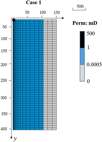
FIGURE 2. Reservoir grid of the numerical model. The blue grids represent the high-permeability region and the gray grids represent the low-permeability region.

Pressure-dependent properties is considered and linearized using the pseudo-pressure and pseudo-time during the derivation of the new analytical solution. It is essential to transform the results obtained with numerical models into production rate over pseudo-time and then fit the transformed results with the derived analytical solution. A comparison of the production rates obtained with the numerical simulation and our analytical model is shown in Figure 3. The blue dotted line indicates the relationship between the gas rate and pseudo-time whereas the red dotted line indicates that determined from the derived analytical solution. The simulation and analytical results agree well. As shown in Figure 3, four flow regimes are identified. Regime 1 exhibits a half-slope straight line in a log-log plot which represents the transient linear flow in region 1. The permeability in this region is relatively high and hence the time constant in this region is relatively short and equals nearly 4 days. Then, the exponential curve of Regime 2 represents the boundary of region 1 is reached, which is referred to as boundary-dominated flow in region 1 or inner-boundary-dominated flow. Regime 3 exhibits the expected straight line with a half-slope signature. In our model, the permeability of region 2 is low and thus the time constant is relatively long (246 days). Regime 4 experiences outer-boundary-dominated flow, which is caused by the boundary of region 2. Table 2 summarizes the four variables after fitting.

FIGURE 3

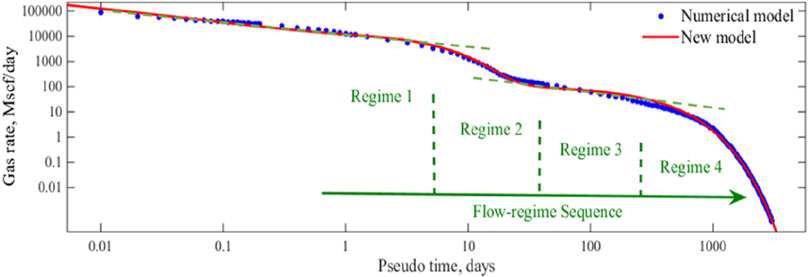
FIGURE 3. Analysis results in Case 1. (Regime 1: transient linear flow in region 1. Regime 2: boundary-dominated flow in region 1. Regime 3: transient linear flow in region 2. Regime 4: boundary-dominated flow in region 2).

TABLE 2

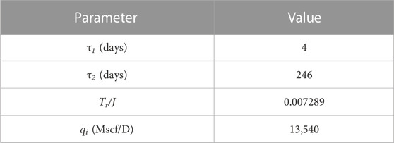
TABLE 2. Model output parameters after fitting.

5.2 Validation for the pore volume ratio

According to Eqs 37, 38 the time constants in region 1 and region 2 are defined to relate strongly with the pore volumes of regions. When Eq. 37 is divided by Eq. 38, we can derive the pore volume ratio of two regions as below:

$\frac{V_{p_2}}{V_{p_1}}=\frac{{\tau }_2}{{\tau }_1}\frac{T_r}{J}(43)$

Substituting the model parameters in Table 2 into Eq. 43, the pore volume ratio can be obtained. We compare it to the given value from the numerical model which is proved correct within the accepted error bound.

$\frac{V_{p_2}}{V_{p_1}}=\frac{246}{4}\times 0.007289=0.44\approx \frac{18}{42}(44)$

The calculated pore volume ratio is nearly equal to the given value in Case 1. To further verify the accuracy of Eq. 43, four more numerical cases are conducted based on the previous numerical model parameters. Table 3 summarizes all the output values from these four numerical cases. Through comparing the given pore volume ratio to the calculated results, the comparison reveals that the accuracy of the calculated results is higher than 95% and thus the model parameters from our new analytical solution can be applied to estimate the pore volume ratio.

TABLE 3

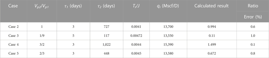
TABLE 3. Summary of model parameters obtained from the four additional numerical cases.

6 Application to field example

In this section, we apply the practical analytical solution to field data. The Mexico gas well is a ‘near textbook’ quality tight gas well with long production history and high quality data, which is operated under a constant bottom-hole pressure of 920 Psi. Several analyses have shown that the reservoir has an ultra-low permeability less than 0.001 md and there is only one well in this field. The original production data is from Blasingame et al. (2007). First, we transform time into the pseudo-time and then the log-log diagnostic plot of gas rate versus pseudo-time is obtained, which exhibit a half-slope straight line and a nearly unit-slope line in Figure 4A indicating linear and boundary-dominated flow. Since the linear flow lasts for nearly 10,000 days, this linear flow regime is identified as Regime 3 and the boundary-dominated flow represents Regime 4. The next step involved matching our model to the production data. The history matching and forecasting results is shown in Figure 4B. The red marks in Figure 4B indicate the production data and the green marks indicate the analytical solution of the history match. A suitable matching degree is revealed. The four model parameters obtained from the history matching process is summarized in Table 4. Based on these output parameters, we forecast the gas rate until 30,000 days, indicated by the black markers in Figure 4B. The more intuitive results are shown in Figure 4C by Cartesian plots. Meanwhile, we can calculate the ratio of region pore volume by Eq. 43 as V_p2/V_p1=104. The ratio can also be used to explain why only two flow regions can be observed rather than four regimes as seen in the previous numerical models. From the ratio, we can obtain that the volume of high permeability region is far smaller than the matrix region and thus the flow in region 1 with high permeability is too fast to be observed.

FIGURE 4

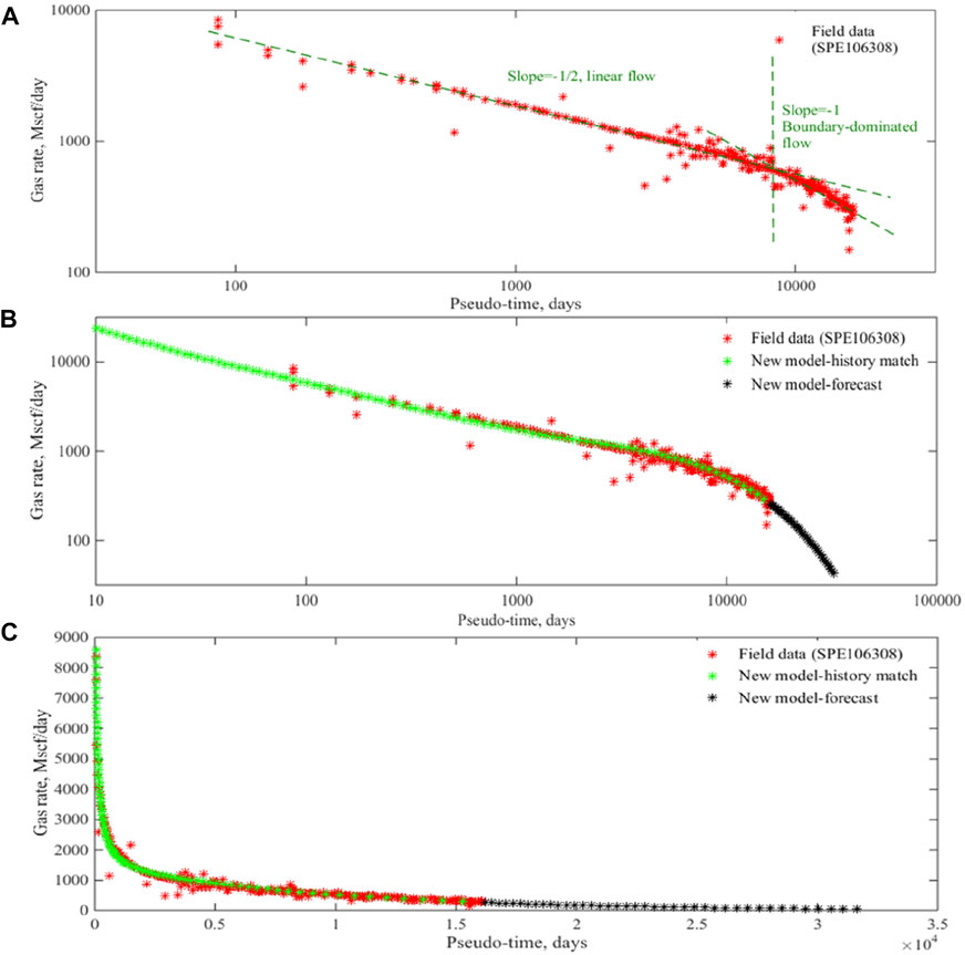
FIGURE 4. Summary of the production profiles in field example. (A) The flow regimes diagnosis. (B,C) The history-matching and forecasting results on a log-log and Cartesian plots.

TABLE 4

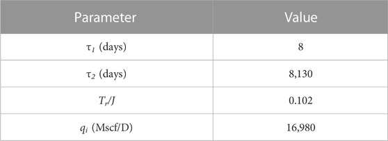
TABLE 4. Model output parameters after fitting.

7 Conclusion

In this paper, a practical analytical model is presented for performance prediction in unconventional gas reservoirs under constant bottomhole pressure. Numerical models were employed to verify the accuracy of derived analytical solution and an excellent agreement was revealed. The following conclusions are drawn:

(1) The proposed analytical solution is derived in real-time domain bypassing Laplace transform and numerical inversion, which is highly suitable for field applications.

(2) Pressure-dependent properties is considered and linearized using the pseudo-pressure and pseudo-time in the analytical model and it is applicable for performance prediction in unconventional gas reservoirs.

(3) The pore volume ratio of different regions can be calculated reversely and the relative error is less than 10%, which is helpful for rapidly evaluating the effect of hydraulic fracturing.

Data availability statement

The original contributions presented in the study are included in the article/Supplementary Material, further inquiries can be directed to the corresponding author.

Author contributions

Conceptualization; methodology and investigation; writing—original draft preparation; project administration; funding acquisition-KQ.

Funding

This study was supported by Basic Research Project from Jiangmen Science and Technology Bureau (Grant No. 2220002000356).

Conflict of interest

The author declares that the research was conducted in the absence of any commercial or financial relationships that could be construed as a potential conflict of interest.

Publisher’s note

All claims expressed in this article are solely those of the authors and do not necessarily represent those of their affiliated organizations, or those of the publisher, the editors and the reviewers. Any product that may be evaluated in this article, or claim that may be made by its manufacturer, is not guaranteed or endorsed by the publisher.

Supplementary material

The Supplementary Material for this article can be found online at: https://www.frontiersin.org/articles/10.3389/feart.2023.1143541/full#supplementary-material

Abbreviations

t, production time, days; ta, pseudo-time, days; $k_{\mathit{1}}$, region 1 permeability, mD; $m_2\left(p\right)$, pseudo-pressure in region 2,psi; $k_2$, region 2 permeability, mD; $T_r$, transmissibility between region 1 and 2, STB/D/psi; $J$, production index, STB/D/psi; $m_1\left(p\right)$, pseudo-pressure in region 1,psi; ${\tau }_1$, region 1 constant time, days; ${\tau }_2$, region 2 constant time, days; ${V_p}_1$, pore volumes of region 1, ft³; $\mu$, fluid viscosity, cp; ${V_p}_2$, pore volumes of region 2, ft³; $\varphi$, porosity; $q_i$, initial production rate, Mscf/D; $C_t$, total compressibility, Psi⁻¹.

References

Abassi, M., Sharifi, M., and Kazemi, A. (2019). Development of new analytical model for series and parallel triple porosity models and providing transient shape factor between different regions. J. Hydrol. 574, 683–698. doi:10.1016/j.jhydrol.2019.04.038

CrossRef Full Text | Google Scholar

Anderson, D. M., and Mattar, L. (2005). “An improved pseudo-time for gas ReservoirsWith significant transient flow,” in Canadian International Petroleum Conference, Calgary, Alberta (Calgary: Society of Petroleum Engineers).

CrossRef Full Text | Google Scholar

Arps, J. J. (1945). Analysis of decline curves. Trans. AIME 160 (01), 228–247. doi:10.2118/945228-g

CrossRef Full Text | Google Scholar

Blasingame, T. A., Amini, S., and Rushing, J. (2007). “Evaluation of the elliptical flow period for hydraulically-fractured wells in tight gas sands -- theoretical aspects and practical considerations,” in SPE Hydraulic Fracturing Technology Conference, College Station, Texas, U.S.A. (College Station: Society of Petroleum Engineers).

CrossRef Full Text | Google Scholar

Blasingame, T. A., McCray, T. L., and Lee, W. J. (1991). “Decline curve analysis for variable pressure drop/variable flowrate systems,” in SPE Gas Technology Symposium (Houston, Texas, USA: Society of Petroleum Engineers).

CrossRef Full Text | Google Scholar

Brown, M., Ozkan, E., Raghavan, R., and Kazemi, H. (2011). Practical solutions for pressure-transient responses of fractured horizontal wells in unconventional shale reservoirs. SPE Res Eval Eng 14 (06), 663–676. doi:10.2118/125043-pa

CrossRef Full Text | Google Scholar

Ci-qun, L. (1983). Exact solution of unsteady axisymmetrical two-dimensional flow through triple porous media. Appl. Math. Mech. 4 (5), 717–724. doi:10.1007/bf02432083

CrossRef Full Text | Google Scholar

Cipolla, C. L., Lolon, E. P., Erdle, J. C., and Rubin, B. (2010). Reservoir modeling in shale-gas reservoirs. SPE Res Eval Eng. 13 (4), 638–653. doi:10.2118/125530-pa

CrossRef Full Text | Google Scholar

Clarkson, C. R. (2013). Production data analysis of unconventional gas wells: Review of theory and best practices. Int. J. COAL Geol. 110, 101–146. doi:10.1016/j.coal.2013.01.002

CrossRef Full Text | Google Scholar

Dejam, M., Hassanzadeh, H., and Chen, Z. (2018). Semi-analytical solution for pressure transient analysis of A hydraulically fractured vertical well in A bounded dual-porosity reservoir. J. Hydrol. 565, 289–301. doi:10.1016/j.jhydrol.2018.08.020

CrossRef Full Text | Google Scholar

Ding, Y., Wu, Y. S., Farah, N., Wang, C., and Bourbiaux, B. (2014). “Numerical simulation of low permeability unconventional gas reservoirs,” in SPE/EAGE European Unconventional Resources Conference and Exhibition (Vienna, Austria: Society of Petroleum Engineers).

CrossRef Full Text | Google Scholar

Duong, A. N. (2011). Rate-decline analysis for fracture-dominated shale reservoirs. SPE Res. Eval. Eng. 14 (03), 377–387. doi:10.2118/137748-pa

CrossRef Full Text | Google Scholar

Fetkovich, M. J. (1980). Decline curve analysis using type curves. J. Pet. Technol. 32 (06), 1065–1077. doi:10.2118/4629-pa

CrossRef Full Text | Google Scholar

Lee, S. T., and Brockenbrough, J. (1983). “A new analytic solution for finite conductivity vertical fractures with real time and Laplace space parameter estimation,” in SPE Annual Technical Conference and Exhibition, San Francisco, California (San Francisco: Society of Petroleum Engineers).

CrossRef Full Text | Google Scholar

Liu, J. H., Lu, M. J., and Sheng, G. L. (2021). Description of fracture network of hydraulic fracturing vertical wells in unconventional reservoirs. Fron Earth S. C. 07, 749181.

CrossRef Full Text | Google Scholar

Ogunyomi, B. A., Patzek, T. W., Lake, L. W., and Kabir, C. S. (2016). History matching and rate forecasting in unconventional oil reservoirs with an approximate analytical solution to the double-porosity model. SPE Res Eval Eng. 19 (01), 070–082. doi:10.2118/171031-pa

CrossRef Full Text | Google Scholar

Qiu, K. X., and Li, H. (2018). A new analytical solution of the triple-porosity model for history matching and performance forecasting in unconventional oil reservoirs. SPE J. 23 (06), 2060–2079. doi:10.2118/191361-pa

CrossRef Full Text | Google Scholar

Rao, X., Xin, L. Y., He, Y. X., Fang, X., Gong, R., Wang, F., et al. (2022). Numerical simulation of two-phase heat and mass transfer in fractured reservoirs based on projection-based embedded discrete fracture model (pEDFM). J. Pet. Sci. Eng. 208, 109323. doi:10.1016/j.petrol.2021.109323

CrossRef Full Text | Google Scholar

Stalgorova, E., and Mattar, L. (2012). “Practical analytical model to simulate production of horizontal wells with branch fractures,” in SPE Canadian Unconventional Resources Conference, Calgary, Canada (Calgary: Society of Petroleum Engineers).

CrossRef Full Text | Google Scholar

Stalgorova, K., and Mattar, L. (2013). Analytical model for unconventional multifractured composite systems. SPE Res Eval Eng. 16 (3), 246–256. doi:10.2118/162516-pa

CrossRef Full Text | Google Scholar

Stehfest, H. (1970). Algorithm 368: Numerical inversion of Laplace transforms [D5]. Commun. ACM. 13 (1), 47–49. doi:10.1145/361953.361969

CrossRef Full Text | Google Scholar

Wattenbarger, R. A., El-Banbi, A. H., Villegas, M. E., and Maggard, J. B. (1998). “Production analysis of linear flow into fractured tight gas wells,” in SPE Rocky Mountain Regional/Low-Permeability Reservoirs Symposium (Denver, Colorado: Society of Petroleum Engineers).

Google Scholar

Wei, S. M., Xia, Y., Jin, Y., Chen, M., and Chen, K. (2019). Quantitative study in shale gas behaviors using A coupled triple-continuum and discrete fracture model. J. Pet. Sci. Eng. 174, 49–69. doi:10.1016/j.petrol.2018.10.084

CrossRef Full Text | Google Scholar

Xia, Y., Jin, Y., Chen, M., and Chen, K. P. (2019). An enriched approach for modeling multiscale discrete-fracture/matrix interaction for unconventional reservoir simulations. SPE J. 24, 1349–1374. doi:10.2118/194012-pa

CrossRef Full Text | Google Scholar