Indications of marine benthos occurrence from multi-spectral multi-beam backscatter data: a case study in the North Sea

To facilitate the conservation of seafloor habitats and planning of offshore activities, there is a growing need for mapping marine benthos in an effective and efficient way. Acoustic data acquired by multi-beam echosounders (MBES) have been extensively used for large-scale and high-resolution seafloor characterization. A deeper understanding of the relationship between backscatter data and sediment compositions can help to identify the benthos occurrence from the MBES data. With two multi-spectral MBES datasets collected near the western Wadden Sea islands in the North Sea, we investigated the potential of mapping marine benthos through backscatter classification. Two unsupervised classification methods, i.e., Bayesian classification, which mainly exploits the backscatter strength from incident angles larger than 20°, and hierarchical clustering of the backscatter strength at different angular ranges, were employed and the results were compared. The classification results from both methods showed a good correspondence with sediment properties such as the median grain size. Moreover, based on a principal component analysis of bottom sample properties, the hierarchical clustering results indicated a better distinction between contributions from the gravel content and benthos occurrence, e.g., sand mason worm density, than Bayesian classification, through involving the backscatter angular variations. Classification for multiple frequencies, on the other hand, showed little difference regarding the relationship with bottom sample properties. Although the backscatter difference between frequencies was also found to positively correlate with certain sample properties, using multi-spectral features for acoustic classification in this study did not reveal additional information compared to single-frequency classification results.

1 Introduction

Knowledge regarding the occurrence of marine benthos is essential for the assessment and conservation of seafloor habitats. Traditional biodiversity monitoring relies on bottom sampling, providing accurate point measurements of the seafloor. However, such methods achieve only sparsely distributed information and are time consuming, especially in the analysis phase. In recent years, acoustic remote sensing technologies such as single-beam echosounders (SBES), sidescan sonars (SSS), and multi-beam echosounders (MBES), have been extensively used for large-scale surveying, producing high-resolution maps (Brown et al., 2011). In particular, MBES have drawn widespread attention to seafloor characterization due to their advantage of simultaneously acquiring bathymetry and backscatter data. By emitting the acoustic signal and beamforming, MBES collect data over a swath, covering a wide range of incident angles. The backscatter strength, which is derived from the received echo intensity, is influenced by the frequency, incident angle, and sediment properties such as interface roughness and volume heterogeneity (Lamarche and Lurton, 2018). Given an acoustic frequency, the angular dependency of backscatter strength is also an intrinsic property of the seafloor (Lurton, 2002; Trzcinska et al., 2021).

The composition of seafloor substrates can give an indication of the associated biological community. The occurrence and bioturbation activity of marine benthos can also have an impact on the sediment properties and affect the backscattering process of acoustic signals as a result (Brown and Collier, 2008). Many studies have pointed out the potential correlation between backscatter strengths, sediment properties, and benthic macrofauna abundance in a specific region (Kostylev et al., 2003; Haris et al., 2012). Using least squares curve fitting and data from a forward-looking sonar, Simons et al. (2007) modeled the backscatter strength at a fixed incident angle as a function of several sediment properties such as gravel percentage. Huang et al. (2018) found that mud content and mean grain size are the most important sediment properties affecting the backscatter strength through a machine learning model random forest decision tree. McGonigle and Collier. (2014), on the other hand, used linear regression to predict mean grain size from the multi-beam backscatter strength. Similarly, Hutin et al. (2005) showed the potential of identifying scallop beds from backscatter strengths using statistical discriminant analysis, but with the combination of SBES data and epi-macrobenthos photographs. Besides the empirical relationship discovered for different regions, a lot of effort has been put in developing quantitative sediment-backscatter models based on well-calibrated MBES data (Lamarche et al., 2011). The widely accepted APL-model (Applied Physics Laboratory, 1994) estimates the backscatter strength at various incident angles for a given median grain size and frequency by assuming a semi-infinite, dissipative, and homogeneous fluid sediment. Having the angular response of calibrated backscatter data, classification of sediment types can be obtained through model inversion (Fonseca and Mayer, 2007; Simons and Snellen, 2008). However, the APL-model is only applicable to a limited range of frequencies up to 100 kHz and absolute backscatter calibration is not always easy to achieve.

Investigation of differences in sediment properties between acoustically defined groups is another important approach of seafloor characterization, in which similar features, e.g., backscatter strength and its derivatives, are assigned to one of several classes. Such methods are usually divided into supervised and unsupervised classification (Brown et al., 2011). Stephens and Diesing (2014) compared six supervised classification techniques on features from bathymetry and backscatter mosaics, stressing the importance of selecting suitable features for mapping seabed substrates. Porskamp et al. (2018) applied a random forest model on MBES data and showed the benefits of using multi-scale features from backscatter mosaics in benthic habitat mapping. Deep learning models also showed the potential for sediment classification given a reliable labeling of the ground truth data (Zhou et al., 2020; Cui et al., 2021). Considering the limitation of backscatter mosaics due to angular normalization, i.e., removing the angular dependence of backscatter strengths, Hasan et al. (2014) demonstrated the importance of angular response features for predicting benthic biota classes, while Alevizos and Greinert (2018) combined the advantage of angular range analysis and multi-dimensional image processing by generating backscatter mosaics with different reference angles. Bayesian classification, introduced by Simons and Snellen. (2009), avoids angular normalization in another way by classifying backscatter strengths from individual beams in an unsupervised manner, which was also adopted and proved effective in the classification of multi-frequency backscatter data (Gaida et al., 2018). The development of multi-spectral MBES brings the opportunity of better distinguishing seafloor substrates (Brown et al., 2019; Gaida et al., 2020a), either by merging single-frequency classification results (Gaida et al., 2018), or by employing features from multiple frequencies as input for classification (Janowski et al., 2018; Misiuk and Brown, 2022). At the same time, a deeper knowledge about the signal penetration and bathymetric uncertainty at different frequencies is required to ensure reliable interpretations (Mohammadloo et al., 2020).

The objective of this study is to investigate the potential of mapping the existence of marine benthos using multi-spectral backscatter data, which is of great importance given the increasing demand for efficient methods of identifying marine benthos for supporting offshore human activities, e.g., offshore windfarm construction, while ensuring a sustainable use of the sea. To this end, two backscatter-based unsupervised classification methods, i.e., Bayesian classification and hierarchical clustering of mean backscatter strengths from different angular ranges, were applied to two datasets acquired by a multi-spectral MBES system in the North Sea. By comparing both methods, we looked into the possibility of achieving additional indications of benthos occurrence through involving the angular information of the backscatter strength. To accomplish this, a principal component analysis (PCA) on bottom sample properties was conducted for exploring the relationship between sediment compositions and backscatter classification results for different frequencies. In addition to comparisons among frequencies, an attempt to use multi-spectral features for acoustic classification was also made, in order to assess the benefits of combining multiple frequencies for our study areas.

2 Materials and methods

2.1 Study areas and datasets

In July and August 2021, two surveys were conducted north of the western Wadden Sea islands, hereafter referred to as “off Ameland and Terschelling” (AT), and “Borkumse Stenen” (BoS), respectively (Figure 1). Both areas had similar water depth, ranging from 22.1 to 29.5 m. There was a trough with gradual slopes in Area AT, whereas Area BoS was shaped around a steep drop in bathymetry, with gradual bathymetric changes in the shallower western region and a more heterogeneous region in the east. During the surveys, an R2Sonic 2026 multi-spectral MBES system was used to collect MBES data at four frequencies, i.e., 90, 200, 300, and 450 kHz, with beam opening angles of 2.3$°$, 1.1$°$, 0.7$°$, and 0.5$°$, respectively. A swath coverage of 130$°$ was adopted. The system settings of the R2Sonic 2026 were kept the same during data acquisition in July and August 2021. In this study, the MBES data were first processed in the QPS software Qimera for bathymetric cleaning and converted into the generic sensor format (GSF). Afterwards, data were separated into different frequencies and input to the backscatter correction algorithm implemented with MATLAB R2020b, in order to extract the beam-averaged backscatter strength (in dB per m² at 1 m) that represents the seafloor properties from the received echo level. For each frequency, the corrected backscatter strength $BS$ was achieved according to

$BS=EL-SL-G-SH-B{P}_T-B{P}_R+TL-10\mathit{log}\left(A\right),$

where $EL$ is the received echo level (dB), $SL$ the source level (dB re 1 μPa at 1 m), $G$ the receiver gain (dB), $SH$ the transducer sensitivity (dB re 1V/µPa). $B{P}_T$ and $B{P}_R$ are the directivity pattern at transmission and reception. $TL$ indicates the two-way sound transmission loss and is calculated as

$TL=2\alpha R+40\mathit{log}\left(R\right),$

where $\alpha$ is the seawater absorption coefficient (dB/m) and $R$ the one-way travel distance (m) of the acoustic signal. In this study, we estimated $\alpha$ using measured water temperature, salinity, and sound speed (Francois and Garrison, 1982a; Francois and Garrison, 1982b). To achieve the backscatter strength in the unit area of 1 m², we also accounted for the ensonified beam footprint area $A$, which is the smaller value between (Amiri-Simkooei, et al., 2009):

$A_p={\mathrm{\Omega }}_{t}R\frac{c{\tau }_{eff}}{2\sin \left({\varphi }_{fl}-{ϵ}_{ac}\right)\cos \left({ϵ}_{al}\right)}$

FIGURE 1

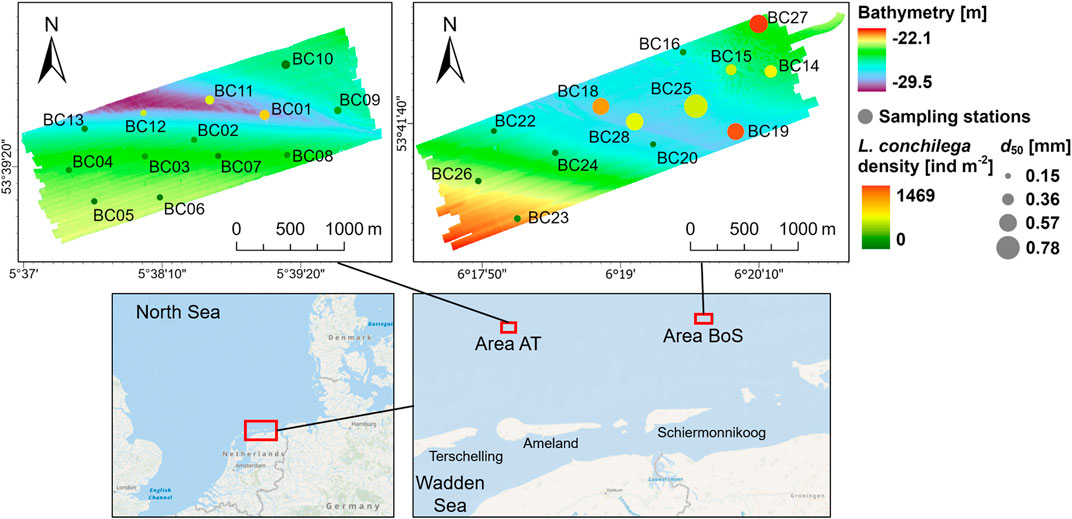
FIGURE 1. Study areas in the North Sea, showing bathymetry, sampling stations, median grain size (d₅₀) and the densities of sand mason worm (Lanice conchilega) in units of individuals per m². Area AT is located north of the islands of Ameland and Terschelling, Area BoS (Borkumse Stenen) in the Borkum Reef Ground.

and

$A_b=R^2{\mathrm{\Omega }}_t{\mathrm{\Omega }}_r,$

where $A_p$ is determined by the beam opening angle for transmission ${\mathrm{\Omega }}_t$ (radians) and the projection of the effective pulse length ${\tau }_{eff}$ (s) on the seafloor. $c$ is the sound speed (m/s). ${\varphi }_{fl}$ is the incident angle (radians) with respect to the flat seafloor. We accounted for the actual seafloor morphology by ${ϵ}_{ac}$ and ${ϵ}_{al}$ (radians), the across- and along-track slope estimated from the bathymetry data via a moving window of 60 pings through a 2D finite difference method. In addition, $A_b$ is determined by the beam opening angles for transmission and reception, ${\mathrm{\Omega }}_t$ and ${\mathrm{\Omega }}_r$. With a beam steering angle $\theta$ (radians), ${\mathrm{\Omega }}_t$ and ${\mathrm{\Omega }}_r$ can be calculated by

$\frac{\lambda }{L\cos \left(\theta \right)},$

Given the signal wavelength $\lambda$ (m) and the array length $L$ (m) (Lurton, 2002).

In both Area AT and BoS, 13 sampling stations were selected for the sediment and macrofauna analysis. At each station, we took 3 bottom samples using a 0.078 m² boxcore. Two replicates were taken for macrofauna analysis, a third for sediment. The macrofauna replicates were sieved on board through a 1 mm mesh in order to extract the fauna from the sediment. Fauna were stored in a 4% formalin solution before analysis in the lab. All animals were counted, but only acoustically hard animals (such as molluscs or the sand mason worm Lanice conchilega) were identified down to species level, other groups only to class or order level. Sediment was analyzed by separating dry weight sieve fractions with mesh sizes of 63, 125, 250, 500, 1,000, 2,000 and 4,000 μm. These fractions were used to determine properties such as median grain size (d₅₀) and weight percentages of gravel, sand, and mud. In addition, volume percentages of shell fragments, living bivalves (the most abundant hard-shell animal), and stones (>4 mm) were determined.

2.2 Bayesian classification

Considering that Area BoS was surveyed only 1 month after Area AT and the sonar settings were kept unchanged, backscatter data from both areas were combined for classification in this study. By doing so, we were able to relate the classification results to a larger number of samples and link the sediment properties of two surveyed areas.

The Bayesian classification method used in this study was developed by Simons and Snellen. (2009). In Bayesian classification, the beam-averaged backscatter strength is regarded as a random variable, which varies only with the seafloor properties for a given frequency and incident angle. As a result of the averaging over many independent scatter pixels within a beam, the obtained backscatter strength per beam is assumed to follow a Gaussian distribution according to the central limit theorem. Here, a scatter pixel indicates the signal footprint, which is the projection of $\tau v$ on the seafloor, with $\tau$ the pulse length and $v$ the sound speed. If there are m sediment types in the surveyed area, the histogram of the backscatter strength at one incident angle can be modeled as a summation of m Gaussian distributions as follows:

$h\left(B{S}_j|\mathit{x}\right)={\displaystyle \sum _{k=1}^m}{c}_k\exp \left[-\frac{{\left(B{S}_j-\overline{B{S}_k}\right)}^2}{2{\sigma }_k^2}\right],$

where $B{S}_j$ represents the backscatter strength of the jth bin in the histogram and $\mathit{x}$ refers to all 3m unknown parameters $\left(\overline{B{S}_1},\dots ,\overline{B{S}_m},{\sigma }_1,\dots ,{\sigma }_m,c_1,\dots ,c_m\right)$. $\overline{B{S}_k}$ and ${\sigma }_k$ are the mean and standard deviation of the backscatter strength for the kth sediment type. In addition, $c_k$ is the weighting factor. The unknown parameters can be determined by solving the non-linear least squares problem

$\min {\displaystyle \sum _{j=1}^M}{\left[n_j-h\left(B{S}_j|\mathit{x}\right)\right]}^2,$

with $n_j$ the number of observations in the jth bin and M the total number of bins in the histogram. In the end, the non-overlapping acceptance region of each sediment type (or Bayes class) is determined by the backscatter strength at the intersections of the m fitted Gaussian distributions according to the Bayesian decision rule for multiple (m) hypotheses given that the a priori probabilities of all m sediment types are equal (Figure 2).

FIGURE 2

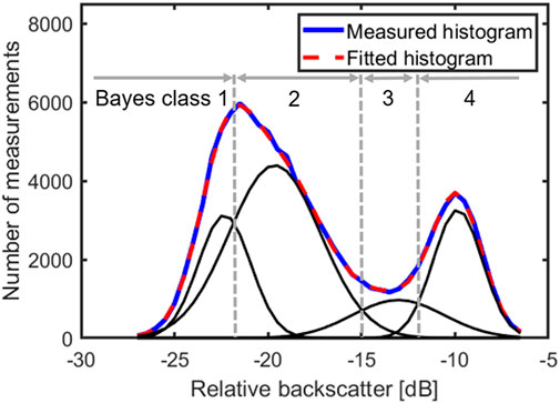
FIGURE 2. An example of acceptance regions for each Bayes class, with the number of sediment types m = 4. The measured and fitted histogram are also illustrated.

To achieve an optimal selection of m, i.e., the number of Bayes classes, we solved the above least squares problem for an increasing number of assumed sediment types, followed by a ${\chi }^2$ goodness-of-fit criterion. The ${\chi }^2$ statistic is calculated as

${\chi }^2={\displaystyle \sum _{j=1}^M}\frac{{\left[n_j-h\left(B{S}_j|\mathit{x}\right)\right]}^2}{n_j},$

assuming Poisson statistics for the random variable $n_j$. This ${\chi }^2$-distributed statistic has $v=M-3m$ degrees of freedom. The goodness-of-fit criterion is further defined as the reduced ${\chi }^2$-statistic (${\chi }_v^2=\frac{{\chi }^2}{v}$). If $v$ is large enough, ${\chi }_v^2$ can also be well approximated by a Gaussian distribution with mean 1 and standard deviation $\sqrt{2/v}$. Therefore, in our implementation, ${\chi }_v^2$ was calculated for each m for a series of incident angles. The iteration of searching for an optimal m stopped when the value of ${\chi }_v^2$ was close to 1 $\pm \sqrt{2/v}$ and not improving anymore.

Beams from larger incident angles contain more scatter pixels, resulting in a Gaussian distribution with a lower standard deviation and thus a higher discrimination ability for sediment types. Considering the robustness of the classification, we first selected several reference incident angles between 40 $°$ and 60 $°$ based on their performance in the ${\chi }^2$ goodness-of-fit and consistency in the fitted Gaussian distributions. Then the average percentage distribution of the acquired acceptance regions at these reference angles was applied to other incident angles. To ensure a similar number of scatter pixels for beams with different incident angles and water depths, we also averaged the backscatter strength over a few adjacent pings and beams (Siemes, 2013). The number of pings was 4 and 3 for the depth range 20–25 m and 25–30 m. The tolerance angle for averaging over beams was 5.0°, 3.2°, and 1.4° for incident angles 20°–25°, 25°–55°, and 55°–65°, respectively. Beams with an incident angle smaller than 20° were excluded in Bayesian classification, since they have too few scatter pixels and therefore the central limit theorem cannot be satisfied.

2.3 Hierarchical clustering of mean backscatter strengths from different angular ranges

After the backscatter correction, the angular variation of the backscatter strength represents an intrinsic property of the seafloor. Although the random fluctuation of the backscatter strength from several individual incident angles is accounted for in Bayesian classification, the angular information is neglected. Therefore, we used a second classification method, in which we looked at the backscatter strength from different angular ranges. We divided incident angles from 0° to 65° into three angular ranges, i.e., near-range (from 0° to 25°), far-range (from 25° to 55°), and outer-range (from 55° to 65°), which is similar to methods used by Fonseca and Mayer. (2007) and the angular range analysis in the Fledermaus Geocoder Toolbox (FMGT) by QPS. Moreover, the half-swath backscatter angular response on the port or starboard side was considered as a unit for feature extraction and classification. Backscatter strengths from each angular range were averaged, resulting in three features (near-mean, far-mean, and outer-mean) for a half-swath angular response. Also, an along-track average over 10 pings was adopted to reduce noise in the backscatter measurements. For each frequency, we constructed a covariance matrix from the three mean backscatter features, on which a PCA was then conducted. We classified data of each frequency separately by inputting the first principal components (PC), which can represent more than 90% of the total variance, to hierarchical clustering (Revelle, 1979) with a Euclidean distance similarity metric and complete linkage algorithm, performed with the built-in function clusterdata() in MATLAB R2020b.

The minimum number of clusters was based on the results of analyzing the Bayesian classification, since Bayes classes include the statistical fluctuations of the backscatter strength. However, as features from a wider angular range were included, it is also possible that the optimal number of clusters/classes was higher in hierarchical clustering. Therefore, for each frequency, starting from the number of Bayes classes, we successively added another cluster during hierarchical clustering to see if a more discriminative classification can be achieved.

2.4 Investigation of classification results using sample properties

The relationship of the detailed sediment composition with the acoustic classes, i.e., Bayes classes or hierarchical clusters, was investigated for 26 bottom samples taken in both area AT and BoS, maximizing the coverage of different sediment types. Nine sample properties (d₅₀, L. conchilega density, total density of molluscs, weight percentages of gravel, sand and mud, volume percentages of stones, dead shells and living bivalves) were considered in the first place. However, we excluded properties showing very high collinearity with others to achieve a better representation of the sample space. We quantified the collinearity using the Variance Inflation Factor (VIF). VIF measures how much the variance of one regression coefficient in a multiple regression model is inflated due to multi-collinearity among predictor variables, and thus can be computed for each predictor. If VIF of one predictor is 1, there exists no correlation between this predictor and the remaining predictors. VIF larger than 10 might indicate a serious collinearity problem, while VIF between 5 and 10 can be cause for concern (Menard, 1995). Based on this, we selected the sample properties iteratively. The one with the highest VIF among 9 properties was first removed. Afterwards, the VIF values were calculated again for the remaining 8 properties. The iteration stopped when the VIF of all included properties were below 5.

On these selected properties for 26 samples in total, a PCA was performed to extract the primary information contained in the sample space. With the first and second PC as two axes, the samples and property vectors can be further displayed together by projecting them onto the span of those two PCs. In this biplot, similar samples will be aggregated together and correlations between properties can be visualized. Specifically, high correlation is indicated by a small angle between two property vectors. This will be further explained in Section 3.3. In combination with the acoustic class corresponding to each sampling station, we were then able to inspect if classifications based on backscatter strengths also revealed differences shown in certain sample properties.

3 Results

3.1 Bayesian classification

Since classification results for the 200 kHz data were very similar to the other two higher frequencies, here we only present the results for 90, 300, and 450 kHz. According to the ${\chi }_v^2$ values and the associated uncertainty, 6, 4, and 4 Bayes classes were selected for 90, 300, and 450 kHz, respectively (Figure 3). Furthermore, several reference incident angles, i.e., 53 $°$ and 54 $°$ for 90 kHz, 43 $°$ and 47 $°$ for 300 kHz, and 43 $°$, 45 $°$ and 51 $°$ for 450 kHz, were chosen for the classification of all incident angles between 20 $°$ and 65 $°$. The classification process was also repeated for two more classes in each frequency, showing that no additional information was brought to the classification maps by adding more Gaussians.

FIGURE 3

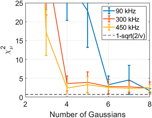
FIGURE 3. ${\chi }_v^2$ values averaged over incident angles from 40° and 60° as a function of the number of Gaussians for the frequencies 90, 300, and 450 kHz.

Compared to the backscatter mosaics (Figure 4), the ascending Bayes class number corresponded to an increase in the backscatter strength (Figure 5). For all frequencies, the highest class occurred in locations with deeper bathymetry, i.e., the trough of Area AT and the eastern seabed of Area BoS. In AT, regions near the sampling station BC04 also fell into a relatively high Bayes class, indicating a pattern that was significant in the backscatter strengths but not found in the bathymetry. Compared to 300 and 450 kHz, Bayesian classification of 90 kHz made additional distinctions for low backscatter strengths, adding extra classes. As for Area AT, although the coverage of classes 1, 2, and 3 in 90 kHz generally aligned with class 1 and 2 in higher frequencies, they had a scattered spatial distribution, likely due to artefacts in the backscatter data caused by rough weather conditions during the measurement. In Area BoS, a small patch of class 2 of 90 kHz near the sampling station BC26 was not observed in other frequencies. Moreover, differences among frequencies existed in the second highest Bayes class. In contrast with higher frequencies, class 5 in 90 kHz was less identified near the trough in Area AT, but distributed slightly more on the eastern side of Area BoS. However, class 3 in 300 and 450 kHz had a broader coverage on the western seabed near the bathymetric drop in the middle of Area BoS.

FIGURE 4

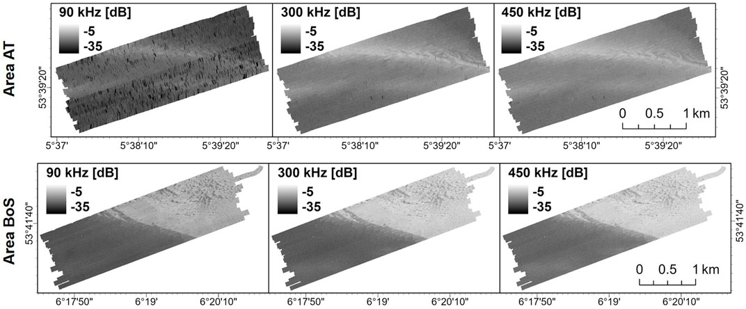
FIGURE 4. Backscatter mosaics (90, 300, and 450 kHz) of both study areas, with the angular variation normalized by the backscatter strength between 40° and 60°.

FIGURE 5

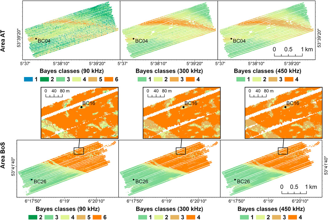
FIGURE 5. Bayesian classification maps for 90, 300, and 450 kHz.

3.2 Hierarchical clustering of mean backscatter strengths from different angular ranges

Guided by the optimal number of classes in Bayesian classification, which was assumed to be the minimum number of classes, 7, 5, and 6 clusters were selected in hierarchical clustering for 90, 300, and 450 kHz, respectively. The classification maps of hierarchical clustering (Figure 6) had a good correspondence with Bayes classes. Especially for 300 kHz, clusters from 1 to 4 indicated similar regions as Bayes classes. Furthermore, cluster 5 revealed a new spatial pattern in Area BoS compared to the Bayesian classification results, corresponding to regions with the highest mean backscatter strengths near the nadir and in the far-range. Such additional information was also found in the hierarchical clusters of 90 and 450 kHz. Moreover, the highest clusters, i.e., cluster 7, 5, and 6 in 90, 300, and 450 kHz, respectively, were not observed in Area AT, which is likely due to a wider range of d₅₀ in Area BoS (see Section 3.3). Cluster 3 in 90 kHz and cluster 1 in 450 kHz were not present in Bayesian classification either. In Area BoS, both clusters corresponded to the low backscatter strengths in the western region, but might be affected by the striped artefacts in the backscatter data. The clustering result of Area AT from 90 kHz was also impacted by rough weather backscatter artefacts, showing several scattered classes. Furthermore, since feature extraction for hierarchical clustering was based on data from half of the surveyed swath, the spatial resolution of the generated classification maps was limited, and variations across track could not be accounted for as in Bayesian classification. Considering regions around the sampling station BC16 in Area BoS, heterogeneous backscatter features in small scales (10–20 m) were discriminated by acoustic classes in Bayesian classification, but could not be resolved in hierarchical clustering (see Figures 5, 6).

FIGURE 6

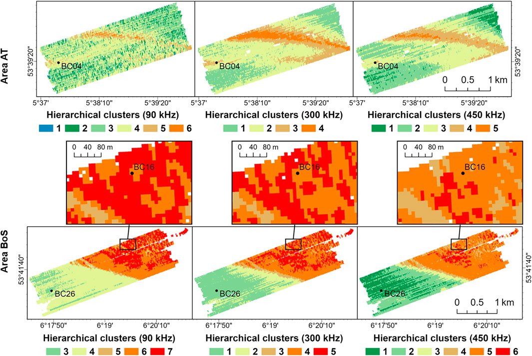
FIGURE 6. Classification maps of hierarchical clustering of mean backscatter strengths from three angular ranges for 90, 300, and 450 kHz.

3.3 Investigation of classification results using sample properties

The sample analysis results showed that the d₅₀ in Area AT ranged from 0.16 to 0.30 mm, indicating a relatively homogeneous composition from fine sand to medium sand. By contrast, Area BoS had a wider range of sediment types from fine to gravelly sand. For both classification methods, the ascending acoustic classes generally corresponded with an increase of d₅₀ (Figure 7). Note that near the sampling station BC16, the sediment had a small median grain size, but the highest acoustic class within 50 m for every frequency, possibly due to a high spatial variation of sediment types shown in that region. According to the Bayesian classification results, BC16 might be located on a small-scale region with softer sediment, while coarser sediment existed in its surroundings (see Figure 5).

FIGURE 7

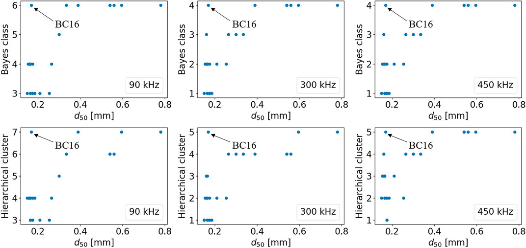
FIGURE 7. Scatter plots of the acoustic classes versus d₅₀. Each dot represents a sampling station, whose classification is determined by the most frequent class within a radius of 50 m around it.

Furthermore, following the process of property selection using the VIF values, L. conchilega density, and the percentages of gravel, sand, mud, dead shells, and living bivalves were finally selected for PCA in the sample space. In the PCA, nearly 70% of the data variability was accounted for by the first two PCs. Moreover, most sample properties, including the percentages of gravel and dead shells and the density of L. conchilega, contributed to the first PC (Figure 8). The L. conchilega density furthermore appeared to correlate positively with the percentages of gravel and dead shells, as indicated by the small angles between their property vectors on the biplot. In contrast, mud and sand were almost uncorrelated considering that their property vectors were nearly perpendicular to each other. BC22 and BC27 showed the least similarity to other samples due to their high percentages of mud and gravel, respectively.

FIGURE 8

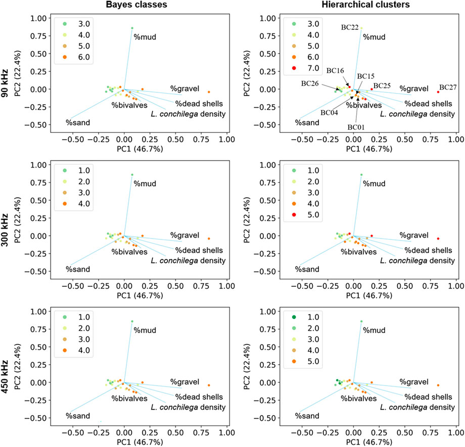
FIGURE 8. PCA biplots with Bayes classes or hierarchical clusters annotated for every sampling station, and the selected properties indicated as vectors. The most frequent acoustic class around each sampling location is indicated by the colors of the dots.

In both the Bayesian classification and hierarchical clustering, the two lowest classes shown in the biplot corresponded well to the close aggregation of samples with a finer sediment and smaller L. conchilega density. However, only the results of 90 kHz showed a clear distinction between the two lowest acoustic classes. Hierarchical cluster 3 in 90 kHz, including locations near BC26 in Area BoS, corresponded with a higher percentage of sand. Sample BC01 from Area AT and BC15 from Area BoS had a similar d₅₀ (around 0.3 mm) and were close in the biplot. Both sampling stations were categorized as the same acoustic class, except for 90 kHz. By contrast, although BC04 (from Area AT) and BC15 (from Area BoS) were even closer in the biplot, BC04 was classified within a lower acoustic class than BC15 for each method and frequency. These two sampling stations differed mostly in their d₅₀, a property not included in the PCA. Due to the high collinearity with other properties, d₅₀ was not considered in the PCA, resulting in its contribution not seen in the biplot.

Differences between Bayesian classification and hierarchical clustering were mostly visible in the biplots for 90 and 300 kHz. For both frequencies, locations in the bathymetrically heterogeneous region in the northeast of Area BoS (BC25 and BC27) were categorized as a higher acoustic class in hierarchical clustering compared to Bayesian classification, consistent with the divergence between the percentage of gravel and both L. conchilega density and the volume percentage of bivalves. Generally, hierarchical clusters indicated the contribution of the gravel content or benthos to the backscatter strengths better than Bayes classes. In the hierarchical cluster map of 450 kHz, a similar spatial pattern was seen for the highest acoustic class as in 90 and 300 kHz. However, due to a more variable distribution of the hierarchical clustering results near BC25 and BC27, both sampling stations did not fall into the highest hierarchical cluster and the difference between the two classification methods in the biplot as mentioned above was absent for 450 kHz.

3.4 Use of multi-spectral features for acoustic classification

Besides the analysis of single-frequency classification results, we observed that the backscatter difference between two frequencies could be an indication of the change in bottom sample properties, such as d₅₀ and L. conchilega density. Considering the similar backscatter strength for 300 and 450 kHz, the backscatter difference between 90 and 300 kHz was taken as an example (Figure 9). The backscatter strength at 300 kHz was lower than at 90 kHz in the near-range, but higher in the outer-range, with the difference up to 4 dB. Far-mean in both frequencies showed less difference. Compared to near-mean, the backscatter difference in far-mean and outer-mean showed particularly a positive correlation with d₅₀ and L. conchilega density, bringing the potential of combining multiple frequencies for sediment classification.

FIGURE 9

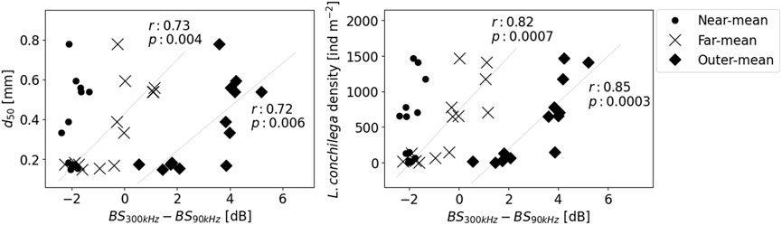
FIGURE 9. Scatter plots of d₅₀ and Lanice conchilega density as a function of the backscatter strength (BS) difference in three angular ranges between 300 kHz and 90 kHz for sampling stations in Area BoS. For far-mean and outer-mean, the correlation between the backscatter difference and sample properties is described by the correlation coefficient r and the associated p-value. Backscatter differences from Area AT are not included considering artefacts at 90 kHz.

Therefore, we also conducted hierarchical clustering on two multi-spectral feature sets, respectively. The first feature set contained mean backscatter strengths from three angular ranges in both 90 and 300 kHz, while the second included only the backscatter difference between 90 and 300 kHz in far- and outer-range. The classification in both cases showed generally the same results as hierarchical clustering for single frequencies, indicating no additional information brought by using multi-spectral features in acoustic classification regarding the MBES data in this study.

4 Discussion and conclusion

Two backscatter-based classification methods, i.e., Bayesian classification and hierarchical clustering of mean backscatter strengths from three angular ranges, were applied to two multi-spectral MBES datasets collected near the western Wadden Sea islands in the North Sea. As an approach extensively used by previous research on various multi-beam backscatter data (Amiri-Simkooei et al., 2009; Simons and Snellen, 2009; Gaida et al., 2018; Koop et al., 2019), Bayesian classification accounts for the statistical fluctuation of backscatter strengths at a certain incident angle and was also proved effective in describing changes of the sediment composition in this study. According to a comprehensive analysis of the sample space through PCA, the resulting Bayes classes generally aligned with the distribution of sample properties. Especially along the first PC in the biplots, the ascending order of Bayes classes appeared to be linked to gravel content and shell fragments, which is consistent with the findings of (Gaida et al., 2020b) based on another relatively homogeneous sandy environment in the Ameland inlet close to Area AT. However, such a relationship between acoustic data and sediment type might change for a more muddy or gravelly seabed (Huang et al., 2018). Besides, the tube-building activity of L. conchilega is known to influence the geoacoustic properties of the sediment such as rigidity and porosity (Ballard and Lee, 2017), allowing an assessment of their occurrence from the backscatter data (Heinrich et al., 2017). In our study areas, regions with a significant density of L. conchilega were also determined as the highest Bayes class, potentially indicating the impact of this species on backscatter strengths.

Regarding the second classification method, the spatial distribution of hierarchical clusters showed a good correspondence with Bayes classes in general. Compared to Bayesian classification, in which only several beam angles around 50 $°$ are used as reference, additional information, e.g., the highest hierarchical cluster, was obtained by considering mean backscatter from different angular ranges in a hierarchical clustering algorithm. With this additional acoustic class shown in the biplots, the contributions of L. conchilega density and volume percentage of bivalves to backscatter were better distinguished from the gravel content and dead shells. Information from the whole angular response curve was also demonstrated to be critical in determining the difference in macrofauna abundance by McGonigle and Collier. (2014). Hasan et al. (2014) stressed the importance of using the mean backscatter strength from 30 $°$ to 50 $°$ when classifying biota including various types of algae and invertebrates. The low number of sampling stations in regions with coarser sediment and higher macrofauna density in our measurements, on the other hand, might limit the ability of predicting biological communities from backscatter data (Brown and Collier, 2008). Also, sediment properties of a local region revealed by bottom samples sometimes did not align with the spatial patterns of acoustic classes in hierarchical clustering results. To account for features from an angular response curve, the finer-scale across-track discrimination was lost in our hierarchical cluster maps due to a limited spatial resolution of the MBES half-swath width.

Among frequencies, differences in the relationship between acoustic classes and the sediment composition were not clearly observed in this study, although small differences could be noticed in the classification maps. Previous research showed a better correlation between backscatter strengths and mean grain size at 30 kHz than 300 kHz regarding a seafloor containing sediment from sand to gravel (Runya et al., 2021). However, for our study areas with mostly sand, this contrast was not observed for 90 and 300 kHz. By further using the backscatter difference at 90 and 300 kHz as features, a combination of multiple frequencies in acoustic classification did not reveal remarkable differences compared to the single-frequency classification results in this study either. For future studies of such a sandy environment, frequencies lower than 90 kHz can be considered to better interpret the coarse sediment distribution and the subsurface properties. Moreover, employing multi-spectral features is still not trivial as it requires determining whether or not the same sediment layer is detected by acoustic signals from multiple frequencies. Investigation on the penetration depth also requires a better understanding of the bathymetry difference between multiple frequencies and the associated bathymetry uncertainties (Schmitt et al., 2008). Considering the underlying link between the seafloor morphology and biological communities (Ellis et al., 2010; Mestdagh et al., 2020; Holzhauer et al., 2022), this can also help to increase the potential of using bathymetry data and its derivatives for characterizing the benthos distribution and improve the interpretation of acoustic classification results.

In summary, although limitations in using the multi-spectral MBES data exist in this study, the approach of linking backscatter classification results to sample properties reveals the potential for mapping the distribution of marine benthos using acoustic measures, especially when taking the angular variation of backscatter strengths into account.

Data availability statement

The raw data supporting the conclusion of this article will be made available by the authors, without undue reservation.

Author contributions

QB implemented the methodology and drafted the original manuscript. SM helped in data collection onboard and bottom sample analysis. SM and MS contributed to the survey planning, provided constructive suggestions for building up the methods, and revised the paper. DGS contributed to the revision of the paper. All authors contributed to the article and approved the submitted version.

Funding

This study was financially supported by the Nederlandse Organisatie voor Wetenschappelijk Onderzoek (NWO), with the project number 18698.

Acknowledgments

The research is part of the NWO-funded project 18698 “Multi-spectral Multi-beam Imaging for Mapping the Occurrence of Marine Benthos”. The authors express their gratitude to the Ministry of Infrastructure and Water Management of Netherlands (Rijkswaterstaat) for their support in the survey planning and measurements on board. Special thanks to Helga van der Jagt, Paula Neijenhuis and Rebecca Bakker (Bureau Waardenburg) for their help on board and their colleagues for sample analyses. The company QPS is thanked for licenses of their software for hydrographic data collection and processing. R2Sonic and Van Oord are also acknowledged for providing the sonar equipment. Finally, the authors would like to thank Boskalis and Deltares for their technical support.

Conflict of Interest

The authors declare that the research was conducted in the absence of any commercial or financial relationships that could be construed as a potential conflict of interest.

Publisher’s note

All claims expressed in this article are solely those of the authors and do not necessarily represent those of their affiliated organizations, or those of the publisher, the editors and the reviewers. Any product that may be evaluated in this article, or claim that may be made by its manufacturer, is not guaranteed or endorsed by the publisher.

References

Alevizos, E., and Greinert, J. (2018). The hyper-angular cube concept for improving the spatial and acoustic resolution of MBES backscatter angular response analysis. Geosciences 8 (12), 446. doi:10.3390/geosciences8120446

CrossRef Full Text | Google Scholar

Amiri-Simkooei, A., Snellen, M., and Simons, D. G. (2009). Riverbed sediment classification using multi-beam echo-sounder backscatter data. J. Acoust. Soc. Am. 126 (4), 1724. doi:10.1121/1.3205397

PubMed Abstract | CrossRef Full Text | Google Scholar

Applied Physics Laboratory (1994). APL-UW high-frequency ocean environment acoustic models handbook. Seattle, WA, USA: University of Washington.

Google Scholar

Ballard, M. S., and Lee, K. M. (2017). The acoustics of marine sediments. Acoust. Today 13, 11–18.

Google Scholar

Brown, C. . J., Beaudoin, J., Brissette, M., and Gazzola, V. (2019). Multispectral multibeam echo sounder backscatter as a tool for improved seafloor characterization. Geosciences 9 (3), 126. doi:10.3390/geosciences9030126

CrossRef Full Text | Google Scholar

Brown, C. J., and Collier, J. S. (2008). Mapping benthic habitat in regions of gradational substrata: An automated approach utilising geophysical, geological, and biological relationships. Estuar. Coast. Shelf Sci. 78 (1), 203–214. doi:10.1016/j.ecss.2007.11.026

CrossRef Full Text | Google Scholar

Brown, C. J., Smith, S. J., Lawton, P., and Anderson, J. T. (2011). Benthic habitat mapping: A review of progress towards improved understanding of the spatial ecology of the seafloor using acoustic techniques. Estuar. Coast. Shelf Sci. 92 (3), 502–520. doi:10.1016/j.ecss.2011.02.007

CrossRef Full Text | Google Scholar

Cui, X., Yang, F., Wang, X., Ai, B., Luo, Y., and Ma, D. (2021). Deep learning model for seabed sediment classification based on fuzzy ranking feature optimization. Mar. Geol. 432, 106390. doi:10.1016/j.margeo.2020.106390

CrossRef Full Text | Google Scholar

Ellis, J. R., Maxwell, T., Schratzberger, M., and Rogers, S. I. (2010). The benthos and fish of offshore sandbank habitats in the southern North Sea. J. Mar. Biol. Assoc. U. K. 91 (6), 1319–1335. doi:10.1017/s0025315410001062

CrossRef Full Text | Google Scholar

Fonseca, L., and Mayer, L. (2007). Remote estimation of surficial seafloor properties through the application Angular Range Analysis to multibeam sonar data. Mar. Geophys. Res. 28, 119–126. doi:10.1007/s11001-007-9019-4

CrossRef Full Text | Google Scholar

Francois, R. E., and Garrison, G. R. (1982a). Sound absorption based on ocean measurements: Part I: Pure water and magnesium sulfate contributions. J. Acoust. Soc. Am. 72, 896–907. doi:10.1121/1.388170

CrossRef Full Text | Google Scholar

Francois, R. E., and Garrison, G. R. (1982b). Sound absorption based on ocean measurements. Part II: Boric acid contribution and equation for total absorption. J. Acoust. Soc. Am. 72, 1879–1890. doi:10.1121/1.388673

CrossRef Full Text | Google Scholar

Gaida, T. C., Mohammadloo, T. H., Snellen, M., and Simons, D. G. (2020a). Mapping the seabed and shallow subsurface with multi-frequency multibeam echosounders. Remote Sens. 12 (1), 52. doi:10.3390/rs12010052

CrossRef Full Text | Google Scholar

Gaida, T. C., Tengku Ali, T., Snellen, M., Amiri-Simkooei, A., van Dijk, T., and Simons, D. (2018). A multispectral bayesian classification method for increased acoustic discrimination of seabed sediments using multi-frequency multibeam backscatter data. Geosciences 8 (12), 455. doi:10.3390/geosciences8120455

CrossRef Full Text | Google Scholar

Gaida, T. C., van Dijk, T. A., Snellen, M., Vermaas, T., Mesdag, C., and Simons, D. G. (2020b). Monitoring underwater nourishments using multibeam bathymetric and backscatter time series. Coast. Eng. 158, 103666. doi:10.1016/j.coastaleng.2020.103666

CrossRef Full Text | Google Scholar

Haris, K., Chakraborty, B., Ingole, B., Menezes, A., and Srivastava, R. (2012). Seabed habitat mapping employing single and multi-beam backscatter data: A case study from the Western continental shelf of India. Cont. Shelf Res. 48, 40–49. doi:10.1016/j.csr.2012.08.010

CrossRef Full Text | Google Scholar

Hasan, R. C., Ierodiaconou, D., Laurenson, L., and Schimel, A. (2014). Integrating multibeam backscatter angular response, mosaic and bathymetry data for benthic habitat mapping. PLoS One 9, e97339. doi:10.1371/journal.pone.0097339

PubMed Abstract | CrossRef Full Text | Google Scholar

Heinrich, C., Feldens, P., and Schwarzer, K. (2017). Highly dynamic biological seabed alterations revealed by side scan sonar tracking of Lanice conchilega beds offshore the island of Sylt (German Bight). Geo-Marine Lett. 37, 289–303. doi:10.1007/s00367-016-0477-z

CrossRef Full Text | Google Scholar

Holzhauer, H., Borsje, B., Herman, P., Schipper, C., and Wijnberg, K. (2022). The geomorphology of an ebb-tidal-delta linked to benthic species distribution and functionality. Ocean Coast. Manag. 216, 105938. doi:10.1016/j.ocecoaman.2021.105938

CrossRef Full Text | Google Scholar

Huang, Z., Siwabessy, J., Cheng, H., and Nichol, S. (2018). Using multibeam backscatter data to investigate sediment-acoustic relationships. J. Geophys. Res. Oceans 123, 4649–4665. doi:10.1029/2017jc013638

CrossRef Full Text | Google Scholar

Hutin, E., Simard, Y., and Archambault, P. (2005). Acoustic detection of a scallop bed from a single-beam echosounder in the St. Lawrence. ICES J. Mar. Sci. 62 (5), 966–983. doi:10.1016/j.icesjms.2005.03.007

CrossRef Full Text | Google Scholar

Janowski, L., Trzcinska, K., Tegowski, J., Kruss, A., Rucinska-Zjadacz, M., and Pocwiardowski, P. (2018). Nearshore benthic habitat mapping based on multi-frequency, multibeam echosounder data using a combined object-based approach: A case study from the rowy site in the southern Baltic Sea. Remote Sens. 10 (12), 1983. doi:10.3390/rs10121983

CrossRef Full Text | Google Scholar

Koop, L., Amiri-Simkooei, A., J. van der Reijden, K., O’Flynn, S., Snellen, M., and G. Simons, D. (2019). Seafloor classification in a sand wave environment on the Dutch continental shelf using multibeam echosounder backscatter data. Geosciences 9 (3), 142. doi:10.3390/geosciences9030142

CrossRef Full Text | Google Scholar

Kostylev, V. E., Courtney, R. C., Robert, G., and Todd, B. J. (2003). Stock evaluation of giant scallop (Placopecten magellanicus) using high-resolution acoustics for seabed mapping. Fish. Res. 60 (2-3), 479–492. doi:10.1016/s0165-7836(02)00100-5

CrossRef Full Text | Google Scholar

Lamarche, G., and Lurton, X. (2018). Recommendations for improved and coherent acquisition and processing of backscatter data from seafloor-mapping sonars. Mar. Geophys. Res. 39, 5–22. doi:10.1007/s11001-017-9315-6

CrossRef Full Text | Google Scholar

Lamarche, G., Lurton, X., Verdier, A. L., and Augustin, J. M. (2011). Quantitative characterisation of seafloor substrate and bedforms using advanced processing of multibeam backscatter—application to cook strait, New Zealand. Cont. Shelf Res. 31 (2), S93–S109. doi:10.1016/j.csr.2010.06.001

CrossRef Full Text | Google Scholar

Lurton, X. (2002). An introduction to underwater acoustics: Principles and applications. 2nd ed. Berlin: Springer.

Google Scholar

McGonigle, C., and Collier, J. S. (2014). Interlinking backscatter, grain size and benthic community structure. Estuar. Coast. Shelf Sci. 147, 123–136. doi:10.1016/j.ecss.2014.05.025

CrossRef Full Text | Google Scholar

Menard, S. (1995). An introduction to logistic regression diagnostics. California: Sage, 66.

Google Scholar

Mestdagh, S., Amiri-Simkooei, A., van der Reijden, K. J., Koop, L., O'Flynn, S., Snellen, M., et al. (2020). Linking the morphology and ecology of subtidal soft-bottom marine benthic habitats: A novel multiscale approach. Estuar. Coast. Shelf Sci. 238, 106687. doi:10.1016/j.ecss.2020.106687

CrossRef Full Text | Google Scholar

Misiuk, B., and Brown, C. J. (2022). Multiple imputation of multibeam angular response data for high resolution full coverage seabed mapping. Mar. Geophys. Res. 43, 7. doi:10.1007/s11001-022-09471-3

CrossRef Full Text | Google Scholar

Mohammadloo, T. H., Snellen, M., and Simons, D. G. (2020). Assessing the performance of the multi-beam echo-sounder bathymetric uncertainty prediction model. Appl. Sci. 10 (13), 4671. doi:10.3390/app10134671

CrossRef Full Text | Google Scholar

Porskamp, P., Rattray, A., Young, M., and Ierodiaconou, D. (2018). Multiscale and hierarchical classification for benthic habitat mapping. Geosciences 8 (4), 119. doi:10.3390/geosciences8040119

CrossRef Full Text | Google Scholar

Revelle, W. (1979). Hierarchical cluster analysis and the internal structure of tests. Multivar. Behav. Res. 14 (1), 57–74. doi:10.1207/s15327906mbr1401_4

PubMed Abstract | CrossRef Full Text | Google Scholar

Runya, R. M., McGonigle, C., Quinn, R., Howe, J., Collier, J., Fox, C., et al. (2021). Examining the links between multi-frequency multibeam backscatter data and sediment grain size. Remote Sens. 13 (8), 1539. doi:10.3390/rs13081539

CrossRef Full Text | Google Scholar

Schmitt, T., Mitchell, N. C., and Ramsay, A. T. S. (2008). Characterizing uncertainties for quantifying bathymetry change between time-separated multibeam echo-sounder surveys. Cont. Shelf Res. 28 (9), 1166–1176. doi:10.1016/j.csr.2008.03.001

CrossRef Full Text | Google Scholar

Siemes, K. (2013). Establishing a sea bottom model by applying a multi-sensor acoustic remote sensing approach. Doctoral dissertation. TU Delft: Uitgeverij BOXPress.

Google Scholar

Simons, D. G., and Snellen, M. (2009). A Bayesian approach to seafloor classification using multi-beam echo-sounder backscatter data. Appl. Acoust. 70 (10), 1258–1268. doi:10.1016/j.apacoust.2008.07.013

CrossRef Full Text | Google Scholar

Simons, D. G., and Snellen, M. (2008). “A comparison between modeled and measured high frequency bottom backscattering,” in Proceedings of the European conference on underwater acoustics (Paris, France: Spinger), 639–644.

CrossRef Full Text | Google Scholar

Simons, D. G., Snellen, M., and Ainslie, M. A. (2007). A multivariate correlation analysis of high- frequency bottom backscattering strength measurements with geotechnical parameters. IEEE J. Ocean. Eng. 32 (3), 640–650. doi:10.1109/joe.2007.891890

CrossRef Full Text | Google Scholar

Stephens, D., and Diesing, M. (2014). A comparison of supervised ClassificationMethods for the prediction of substrate type using multibeam acoustic and legacy grain-size data. PLoS One 9 (4), e93950. doi:10.1371/journal.pone.0093950

PubMed Abstract | CrossRef Full Text | Google Scholar

Trzcinska, K., Tegowski, J., Pocwiardowski, P., Janowski, L., Zdroik, J., Kruss, A., et al. (2021). Measurement of seafloor acoustic backscatter angular dependence at 150 kHz using a multibeam echosounder. Remote Sens. 13 (23), 4771. doi:10.3390/rs13234771

CrossRef Full Text | Google Scholar

Zhou, P., Chen, G., Wang, M., Chen, J., and Li, Y. (2020). Sediment classification of acoustic backscatter image based on stacked denoising autoencoder and modified extreme learning machine. Remote Sens. 12 (22), 3762. doi:10.3390/rs12223762

CrossRef Full Text | Google Scholar